
Which Curve Fits Best: Fitting ROC Curve Models to Empirical Credit-Scoring Data

Faculty of Management and Economics, Gdańsk University of Technology, 80-233 Gdańsk, Poland
Risks 2022, 10(10), 184; https://doi.org/10.3390/risks10100184
Submission received: 30 June 2022
/
Revised: 12 September 2022
/
Accepted: 14 September 2022
/
Published: 20 September 2022
(This article belongs to the Special Issue Data Analysis for Risk Management – Economics, Finance and Business)
Abstract
:In the practice of credit-risk management, the models for receiver operating characteristic (ROC) curves are helpful in describing the shape of an ROC curve, estimating the discriminatory power of a scorecard, and generating ROC curves without underlying data. The primary purpose of this study is to review the ROC curve models proposed in the literature, primarily in biostatistics, and to fit them to actual credit-scoring ROC data in order to determine which models could be used in credit-risk-management practice. We list several theoretical models for an ROC curve and describe them in the credit-scoring context. The model list includes the binormal, bigamma, bibeta, bilogistic, power, and bifractal curves. The models are then tested against empirical credit-scoring ROC data from publicly available presentations and papers, as well as from European retail lending institutions. Except for the power curve, all the presented models fit the data quite well. However, based on the results and other favourable properties, it is suggested that the binormal curve is the preferred choice for modelling credit-scoring ROC curves.
1. Introduction
In this paper, we discuss the modelling of receiver operating characteristic (ROC) curves in the domain of credit scoring. Over the last three decades, the retail lending world has transformed into a sophisticated, data-driven industry with automated processes and statistical tools. In a challenging environment where the danger of rising inflation, impending recession, repercussions of the COVID-19 pandemic and the Russo-Ukrainian war (to name only the most apparent risk factors) threaten the stability of the financial sector, a solid foundation of accurate data and proper tools seems even more needed.
Credit scoring is one of the most successful implementations of machine learning in finance. It is used to produce a numerical assessment of a customer’s probability of not repaying the loan. Various tools are used to build credit-scoring models (scorecards), including logistic regression, decision trees and neural networks (Anderson 2007). The discriminatory power of a scoring model is usually assessed by the measures summarising its ROC curve.
ROC curve models are discussed in the literature primarily in the context of biostatistical applications. However, they may also prove to be a valuable tool in credit-risk management. As discussed in the literature section, credit-risk practitioners and researchers might need such models, for example, to estimate the AUROC (the area under the ROC curve) on a sample basis or to better understand the shape of the curve and its implications for credit decisions. In credit management practice, the need to model ROC curves also arises when one wants to assess the impact of the credit scorecard that is yet to be built. For example, a lender knows that an analyst team can produce a new scorecard with a Gini coefficient 15% higher than the current one. This new scorecard may be based on newly available data or may be developed using a new classification methodology. The question arises: to what extent introducing the scorecard can reduce credit losses or increase the profitability of the loan portfolio. Using the ROC curve models presented in the following sections, one can easily draw the expected ROC curve and perform the appropriate calculations.
The main goal and contribution of our work is to review the ROC curve models proposed in the literature, primarily in medical sciences and biostatistics, to reformulate them, if necessary, so that they better reflect credit-risk-management needs, and to fit them to real-life credit-scoring ROC data in order to determine which of the curve models fits the empirical data best and could be used in the practice of credit-risk management. The novelty of this paper is the discussion of theoretical ROC curves from the perspective of credit scoring. Not many authors mention theoretical ROC curve models within the domain of credit-risk management. Satchell and Xia (2008), Kürüm et al. (2012) and Kochański (2021) are notable exceptions. To the best of our knowledge, this article constitutes the first attempt to systematically test a set of ROC curve models against empirical data related to credit scoring. We not only perform the quantitative analysis, but also provide arguments that are not purely quantitative for choosing ROC curve models that best serve credit-risk management.
The next section provides a brief literature background. Then, we present several theoretical models for an ROC curve and describe them in the credit-scoring context. The model list includes the binormal, bigamma, bibeta, bilogistic, power, and bifractal curves. The models are then tested against empirical credit-scoring ROC data found in publicly available publications or obtained from European credit institutions. We show that except for the power curve, all the presented models fit the data quite well. However, based on the results and the discussion of the additional properties of the models, we suggest that the binormal curve should be treated as the preferred choice for modelling credit-scoring ROC curves.
2. Literature Background
The literature on ROC curves is extensive, but most of it comes from areas not related to credit risk. This is not surprising as ROC curves derive from signal-detection theory (Wichchukit and O’Mahony 2010; Swets 2014). They are currently popular in many domains as a method to graphically present the separation power of binary classifiers (Fawcett 2006). Examples of such binary classifiers include diagnostic tests and biomarkers in biostatistics (Hajian-Tilaki 2013; Mandrekar 2010; Faraggi et al. 2003; Cook 2007), detectors in signal processing (Bowyer et al. 2001; Atapattu et al. 2010), credit scores in banking (Blöchlinger and Leippold 2006; Thomas 2009; Anderson 2007), and, generally, binary classification models in machine-learning applications (Hamel 2009; Guido et al. 2020).
An ROC curve plots the true-positive fraction against the false-positive fraction as the cut-off point varies (Metz 1978; Krzanowski and Hand 2009). Depending on the domain, the true-positive and the false-positive fractions may be referred to as a detect rate and false-alarm rate in signal processing (Levy 2008; Chang 2010), as sensitivity and 1-specificity in biostatistics (Park et al. 2004), or as a cumulative bad and good proportion in credit scoring (Thomas 2009).
An ROC curve can be summarised with its “area under the curve” (AUC or AUROC) index (Bamber 1975; Bradley 1997; Bewick et al. 2004), also called a c-statistic or a c index (Cook 2008). The AUROC measures the discrimination power of the binary classifier. Generally, with some reservations related to uncertainty (Pencina et al. 2008), the shape of the curve (Idczak 2019; Řezáč and Koláček 2012) as well as to the cost of misclassification (Cook 2007; Hand 2009), the higher the AUROC, the better. Plotting the ROC curve for a scorecard is not a necessity. Some researchers propose alternative approaches (e.g., Hand 2009), but the ROC curve is considered standard practice by credit-risk professionals (Anderson 2007; Thomas et al. 2017; Siddiqi 2017). Credit-scoring researchers and practitioners frequently use the AUROC to assess, improve, and compare scorecards (Djeundje et al. 2021; Tripathi et al. 2020; Xia et al. 2020; Shen et al. 2021; Lappas and Yannacopoulos 2021).
In the credit-scoring domain, the Gini coefficient, which, in fact, is a rescaled AUROC, is often used by the practitioners (Thomas et al. 2017, p. 191; Řezáč and Řezáč 2011):
It should be noted that the Gini coefficient is equivalent to a special case of Somers’ D statistic where one of the associated variables (the target/response) is binary (0/1) and the other one (the classifier) is at least ordinal (Somers 1962; Thomas et al. 2017, p. 189).
If the classifier function and the data set are given, then the empirical ROC curve is uniquely determined. However, an ROC curve model, i.e., a mathematical formula approximating the curve, may be needed in certain circumstances. The literature examples of such situations include (1) the sample-based inference and estimation of AUROC, (2) the ROC curve shape description, and (3) the simulation of the ROC curve when data are absent or scarce.
(1) The use of ROC curve models to estimate the AUROC is widespread, primarily in biostatistics. With the ROC curve model, the path of the curve can be estimated based on sample results, and the confidence intervals for the AUROC may be computed (Lahiri and Yang 2018; Gonçalves et al. 2014; Hanley 1996; Faraggi and Reiser 2002). Satchell and Xia (2008) discussed using the analytic models for ROC curves in the credit-scoring context. They claimed that the theoretical ROC curves are helpful, especially when the sample size of bad customers is small, as the models help increase the accuracy of the AUROC estimation. Indeed, the scarcity of data usually drives the need for such models. Some of the formulas described in this paper were derived in this context and serve as the basis for such an estimation (Hanley 1996; Bandos et al. 2017; Mossman and Peng 2016).
(2) Knowing the area under the curve turns out to be insufficient, especially when one takes no account of its shape. Janssens and Martens (2020) discussed the importance of ROC curve shapes in medical diagnostics. Hautus et al. (2008) utilised the binormal model to demonstrate how the shape of the ROC curve relates to the same–different sensory tests in the food industry. Omar and Ivrissimtzis (2019) fitted the theoretical ROC bibeta curve to the results of machine-learning models in order to show that such an approach provides additional insight into the behaviour at the ends of the ROC curves. Řezáč and Koláček (2012) and Idczak (2019) showed that, depending on the shape, some credit-scoring models excel at distinguishing the best customers from good ones, while others are preferred if a lender intends to exclude the worst loan applicants. A practical example of such an analysis was provided by Tang and Chi (2005); the model with a much lower AUROC still outperformed the competing, high-AUROC model in terms of the accuracy in classifying the best customers.
Another example when information about the shape of an ROC curve is needed is a situation when the data are censored or “truncated” (Scallan 2013), i.e., a lender does not have good/bad information on rejected applicants. Models for ROC curves could enable the modelling of the unknown portion of the curve.
Not taking the shape of the ROC curve into account when summarising it with the AUROC was raised as one of the major deficiencies of an ROC analysis, which led to proposing alternative measures such as Hand’s h-measure. (Hand 2009; Hand and Anagnostopoulos 2013).
(3) Occasionally, a credit-risk manager might need to draw ROC curves when data are absent or scarce (for example, when a scorecard is yet to be built). In this context, Kürüm et al. (2012) showed how to use the binormal approximation to optimise the AUROC of the model for a set of corporate loans where the number of bad customers was limited. Outside the domain of credit scoring, Lloyd (2000) provided an extreme example of an inference from limited data. He estimated ROC curves from one data point per curve, assuming that the ranking function (equivalent to credit scoring in finance) was an unobserved latent variable. Of course, such an inference would not be possible without the ROC curve models (binormal model in this case).
In the literature, many models for ROC curves have been suggested. Most of the propositions come from medical statistics. The most frequently used model is the binormal curve (Hanley 1996; Metz 1978) and its modifications (Metz and Pan 1999). Other models include the bibeta (Chen and Hu 2016; Gneiting and Vogel 2022; Mossman and Peng 2016; Omar and Ivrissimtzis 2019), bigamma (Dorfman et al. 1997), bilogistic (Ogilvie and Creelman 1968), power curve (Birdsall 1973) and exponential/bifractal model (England 1988; Kochański 2021). These models will be discussed in more detail in the following section. We found no systematic review where multiple ROC curve models were fitted to the same data, be it medical data or data from any other field. However, a few papers discussed the empirical goodness of fit of particular models. For example, Swets (1986) claimed that in many empirical cases the binormal model turns out to have a good fit, and Gneiting and Vogel (2022) showed that the bibeta model fits better than the binormal one, especially under the assumption of a concave ROC curve.
Note that in the following text, the credit-scoring nomenclature is used. The binary classifier in question is the credit scoring; the observed values of the classifier are referred to as the credit scores, positives (signal, hits, cases) are “bads” or “bad customers’”, negatives (noise, false alarms, controls) are “goods” or “good customers”, etc. In line with the practice in credit-risk management, the Gini coefficient is preferred over the AUROC as the summary statistic of an ROC curve.
Before we go any further, one thing needs to be clarified to avoid confusion. Despite the similarity of some names, ROC curve models and classification models are completely different animals. The latter are basically classification functions that return predictions or rankings (such as credit scores). When applied to data sets, the ranking functions generate empirical ROC curves. The ROC curve models, on the other hand, are approximations of the shape of ROC curves. If we find that, for example, the bilogistic curve best approximates the ROC curve of the scoring model, then it does not mean that the logistic regression was, or should be, used to develop the model. On the contrary, the ROC curve generated by logistic regression may be best approximated by the bibeta function, and the bilogistic model may prove to have the best fit when a neural network or support vector machine is used.
3. ROC Curve Models
One way to look at an ROC curve is to view it as a function [0; 1]→[0; 1] built using two cumulative distribution functions. In the context of credit scoring, these two CDFs are those of the credit scores for good and bad customers. The general formula for an ROC curve is then (Gönen and Heller 2010):
where FB is a CDF of the scores of bad customers, FG is a CDF of the scores of good customers, and is its inverse.
where s denotes the value of the test, that is, the score or its monotone transformation. Several ROC curve models proposed below take advantage of this simple observation: it may be assumed that the two CDFs follow specific probability distributions.
Equation (2) shows that an ROC curve is invariant to monotone transformations of the underlying scores; the score does not go directly to the ROC equation, only the CDFs do. Therefore, in the following text, the “scores” may refer to the scores themselves or to their monotone transformations.
3.1. Bibeta and Simplified Bibeta Models
If the scores for bad borrowers are distributed according to a beta distribution with parameters αB and βB and the scores for good customers follow Beta(αG,βG), then the formula for the ROC curve is
where FαB,βB and FαG,βG are CDFs of the two beta distributions (Gneiting and Vogel 2022; Omar and Ivrissimtzis 2019). Such a model could be called a “bibeta” ROC curve. The bibeta model that has been used in several articles (Chen and Hu 2016; Mossman and Peng 2016) is a simplified version of the above equation, where αB = 1 and βG = 1. Then:
and
so, the formula for the bibeta ROC curve is reduced to the following:
In this paper, the curve generated by (7) will be called the “simplified” bibeta.
3.2. Bigamma Model
The “bigamma” model (Dorfman et al. 1997), by analogy, assumes that the scores, or some monotone transformation of them, follow two gamma distributions:
Note that Dorfman et al. (1997) proposed that αB = αG, βB = 1 and 0 < βG ≤ 1, but these restrictions are not included in this article, because they resulted in a much worse fit in the preliminary calculations.
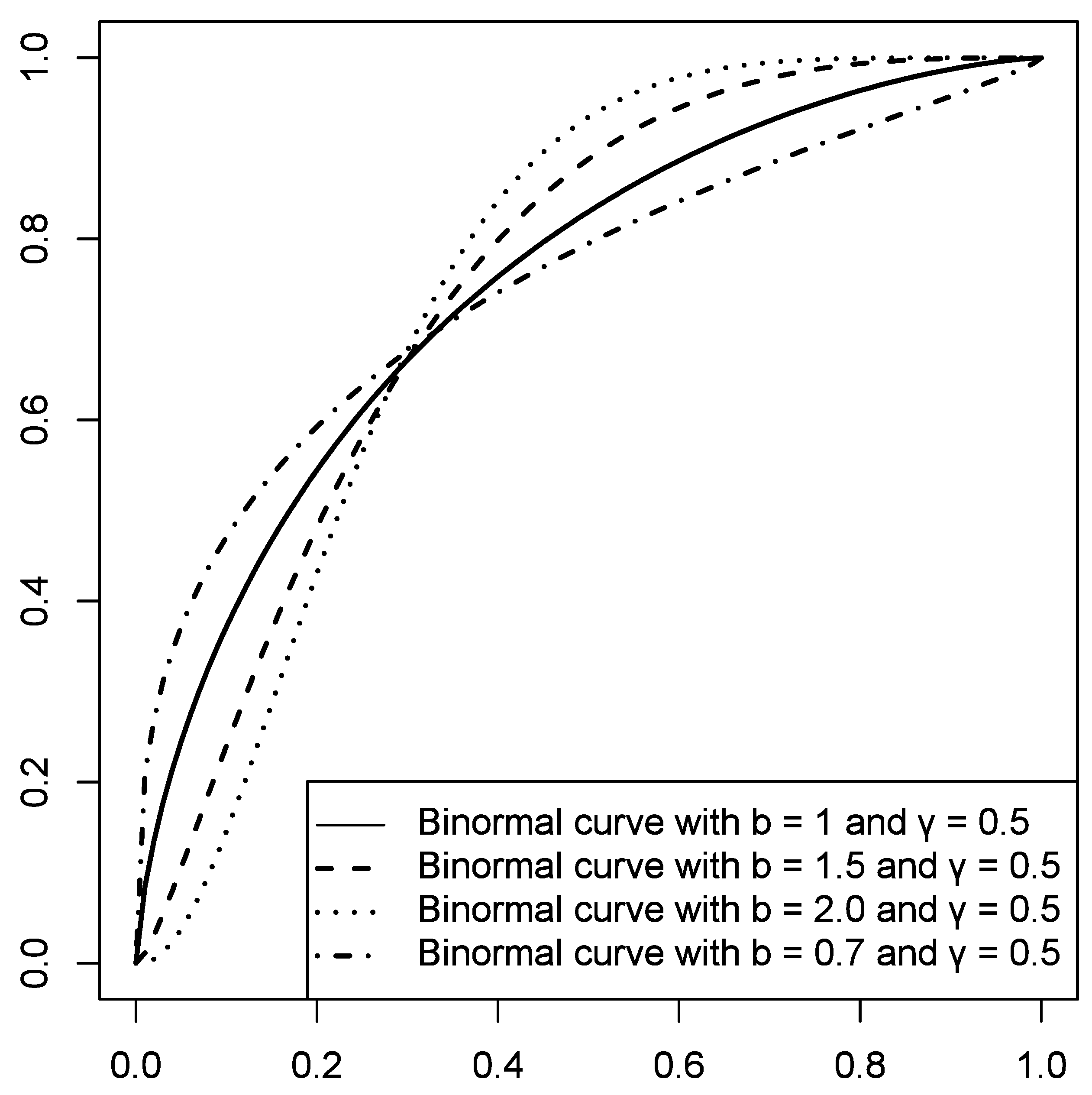
3.3. Binormal Model
The same analogy could be used to build the binormal model:
Equation (9) has four parameters, but it can be rewritten in an equivalent form with just two parameters:
where Φ is a CDF of a standard normal variable, Φ−1 is its inverse and a equals the distance between the mean scores of goods and bads measured in terms of units of s.d. of the good scores:
and b is the ratio between the standard deviations of the bad and good scores:
3.4. Bilogistic Model
There is also another perspective of the binormal model. Φ may be viewed as a (probit) link function in the more general equation for an ROC curve:
where g( ) is a link function. Taking such a perspective, we can select another link function. If a logit function is taken:
the bilogistic ROC curve model is derived. After several transformations, the formula for the bilogistic curve looks as follows:
The Formula (15) will be used as the bilogistic model in the next section.
All the curves discussed before the bilogistic model are examples of parametric ROC curve models, where one starts with distributions and then arrives at the formula. The bilogistic curve can be viewed as an “algebraic” ROC curve model, where the underlying distribution is somewhat “secondary” to the formula itself.
3.5. Power Function
A simple example of a purely algebraic model is the “power function” (Birdsall 1973, p. 138):
The power function can also be derived as the “Lehmann ROC curve” based on proportional hazards specification (Gönen and Heller 2010). From a credit-scoring perspective, the power ROC curve has an attractive property, which could be called “fractal” (Kochański 2021). If the shape of an ROC curve follows Equation (16), and if we take any fraction of the lowest-scored customers and graph the ROC curve for this group, then the shape of the ROC curve remains the same. The AUROC also remains constant: AUROC = 1/(1 + θ), as well as the Gini coefficient: Gini = (1 − θ)/(1 + θ). If one would like to make the Gini coefficient an explicit function parameter, one could reformulate Equation (16) in the following way:
where γ is a parameter for the Gini coefficient.
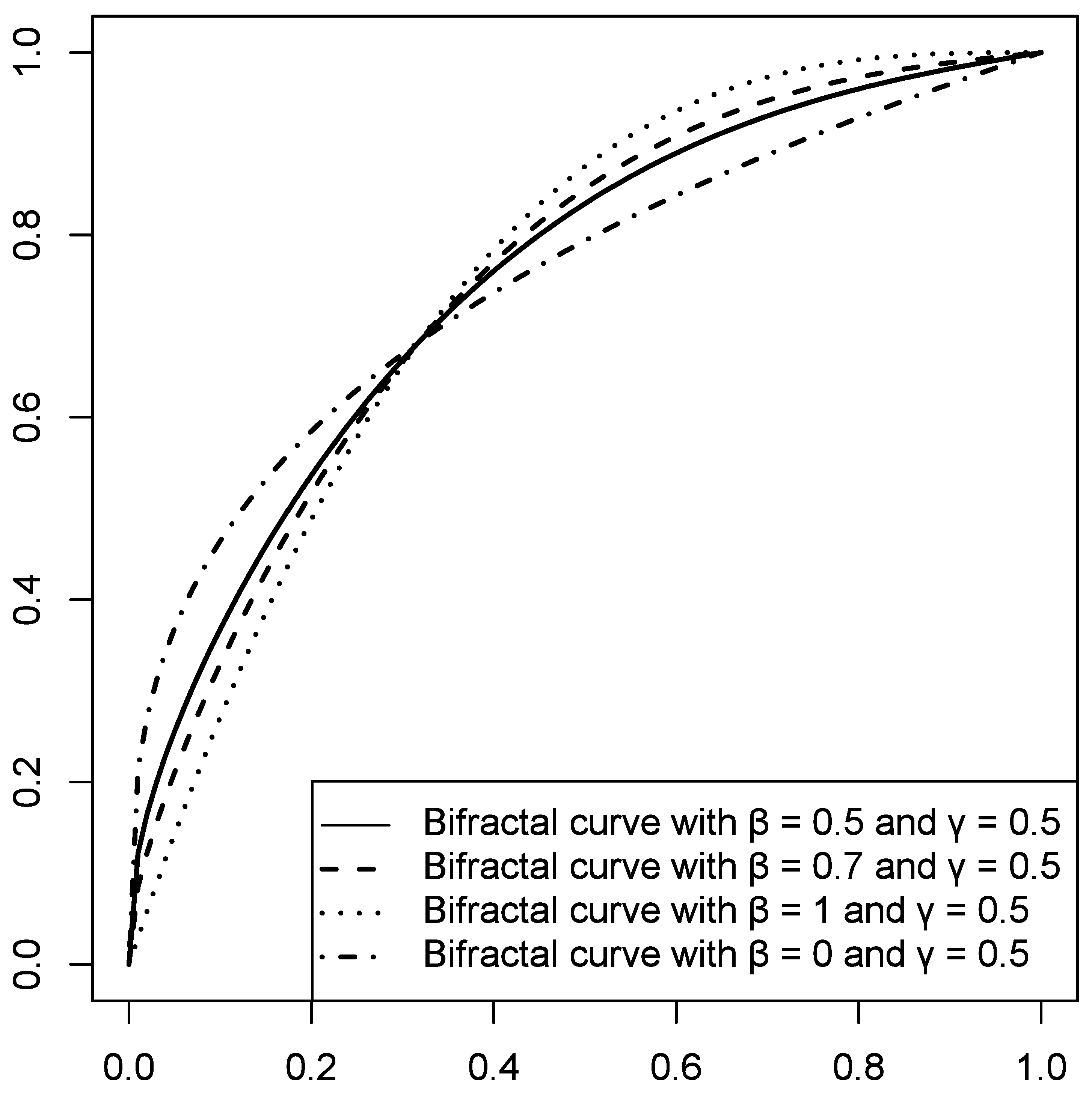
3.6. Bifractal Model
Kochański (2021) proposed a function that keeps the shape (and the AUROC/Gini) when plotted for any fraction of the highest-scored customers:
and showed that the empirical ROC curves lie somewhere between those two extremes. This observation prompted the development of the “bifractal” model:
as a linear combination of the two “fractal” curves. The analogous formula was also experimentally found to provide a good fit and was referred to as “exponential ROC” or EROC by England (1988).
The apparent advantage of the bifractal function in Equation (19) is that it contains the Gini coefficient as its explicit parameter. Moreover, the other parameter of the bifractal ROC curve has a meaningful and intuitive interpretation as a distance between the two fractal curves.
3.7. Reformulated Binormal and Midnormal Models
An explicit Gini coefficient could be a decisive advantage of the bifractal compared to other models. However, as it turns out, the binormal curve function may also be reformulated, and we may obtain a function with the Gini coefficient as a parameter. Thanks to a simple analytic formula for the area under the ROC curve (Bandos et al. 2017):
Equation (10) transforms so that now the formula has the Gini coefficient as its parameter (γ):
The explicit Gini coefficient in the formula seems essential for the modelling. Consequently, the parametric form of the binormal model described by Equation (21) will be used for empirical curve fitting in the next section.
Older works have also described a simplified version of the binormal model (this simplified version is sometimes referred to as the “normal” curve). This model is based on the assumption of the equal variances of the underlying score distributions of good and bad observations (Swets 1986). As a consequence, the b parameter equals 1, and Equation (21) is transformed to:
Such a model has only one parameter, the Gini coefficient, and will here be referred to as the “midnormal” model.
3.8. Midfractal Model
Similarly, one can reduce the bifractal model (Equation (19)) to a one-parameter curve by setting β to 0.5 (in the middle of the two fractal curves):
Again, this curve has only one parameter γ, which stands for the Gini coefficient. This curve will here be referred to as the “midfractal” model.
4. Fitting ROC Curve Models to Empirical Data
The theoretical models for an ROC curve presented in the previous section can be fitted to the empirical ROC data of real-life scoring models in credit institutions. For the empirical analysis presented below, two types of sources of ROC curve data were used: (1) research/industry articles and presentations and (2) data from credit institutions obtained under an anonymity condition.
- (1)
- We used the following papers containing data or at least graphs of empirical ROC curves related to credit scoring: Řezáč and Řezáč (2011), Wójcicki and Migut (2010), Hahm and Lee (2011), Iyer et al. (2016), Tobback and Martens (2019), and Berg et al. (2020). Additionally, presentations by Jennings (2015) and Conolly (2017) were used. To obtain the numbers (x and y coordinates of the points that make up the empirical ROC) in some cases, it was necessary to read the data from the graph itself; therefore, an online tool was used to transform graphs into numbers by pointing and clicking.
- (2)
- Four retail lenders in Europe shared the empirical ROC curves of their credit-scoring models. The data were provided under the condition of anonymity. These models are presented in this article under the symbols A1, A2, B1, B2, B3, C1, and D1.
All the empirical curves in the analysis reflect the discrimination characteristic of some form of a credit-scoring model; the only exception is the antifraud model from Wójcicki and Migut (2010), where the target variable is a fraudulent loan, not a default. The empirical ROC curves describe scoring models that are created using various methods, including support vector machines (Tobback and Martens 2019) or a proprietary methodology (Jennings 2015), but the dominant approach is logistic regression in various forms (Hahm and Lee 2011; Řezáč and Řezáč 2011; Wójcicki and Migut 2010; Berg et al. 2020). In the case of the data coming from the four credit institutions, we do not have information about the methods used to develop the scoring models.
Once the data are available, the question emerges: What is the adequate procedure for fitting the curve? The binormal and bilogistic curves may be fitted quite intuitively through a probit/logit transformation and a simple linear-regression fitting (Swets 1986), and the parametric ROC curve models may be fitted with maximum-likelihood procedures (Metz and Pan 1999; Ogilvie and Creelman 1968). Such a procedure is not available for algebraic models (such as the bifractal curve or power function). As it is reasonable to use the same fitting method for all the ROC curve models, we applied the minimum distance estimation (MDE) method as developed by Hsieh and Turnbull (1996) and Davidov and Nov (2012), and described by Jokiel-Rokita and Topolnicki (2019). We used the numerical optimisation in R (optim function from the R stats package). The “objective function” to be minimised is the L2-distance measure between the empirical ROC curve and the theoretical ROC curve function (Jokiel-Rokita and Topolnicki 2019):
where is the empirical ROC curve (piecewise linear interpolation of empirical ROC data points) and is the ROC curve model with as a vector of parameters (1–4 parameters depending on the function). The minimal distance estimator of the parameter vector is defined by:
As a result of the choice of such an objective function, the average vertical root-mean-square distance between the empirical curve and the theoretical curve was minimised.
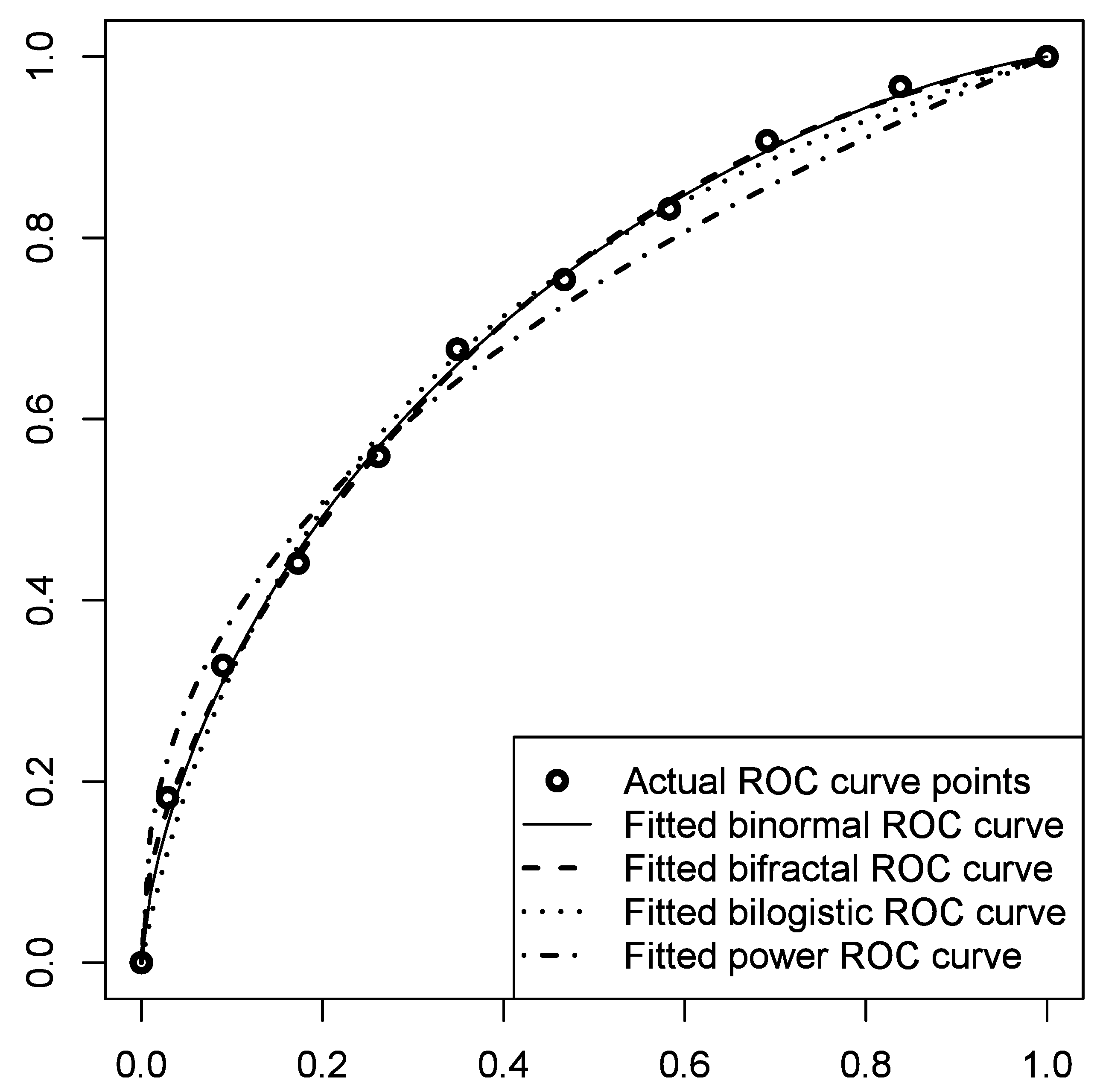
Before we provide the summary results based on all the curve models and all the ROC data sets gathered, let us introduce an illustrative example. The example results of fitting four curves (bifractal, binormal, bilogistic, and power) to the empirical ROC curve obtained for the purposes of this study from an anonymous credit institution (D1) are presented in Figure 3 and Table 1. As it can be seen, the binormal and bifractal models fit the data quite well. At the same time, the highest deviation was observed in the case of the power curve. Moreover, the Gini coefficient implied by the power curve differed slightly from the Gini coefficient implied by the first two models (and also differed from the actual underlying Gini coefficient, which was circa 0.43).
Table 2 presents the goodness of fit for all the data sets gathered. For reasons of clarity, the square root of the minimised objective (fobj) was multiplied by 100; note that it can then be interpreted as the average (root mean squared) vertical distance between the empirical ROC curve and the fitted ROC curve, expressed in percentage points. As it turns out, the binormal model was the best in terms of goodness of fit in 10 cases. On average, the vertical distance between the empirical and binormal ROC curves was less than one percentage point and in the worst case it did not exceed two points, which could be considered an excellent fit. The bibeta model won in five instances. The bilogistic model, which on average fit slightly worse than the competing models, was the best in four cases. The bifractal model also showed a good fit, but it was worse than the binormal in all but one case. The power curve showed the worst fit, with one exception.
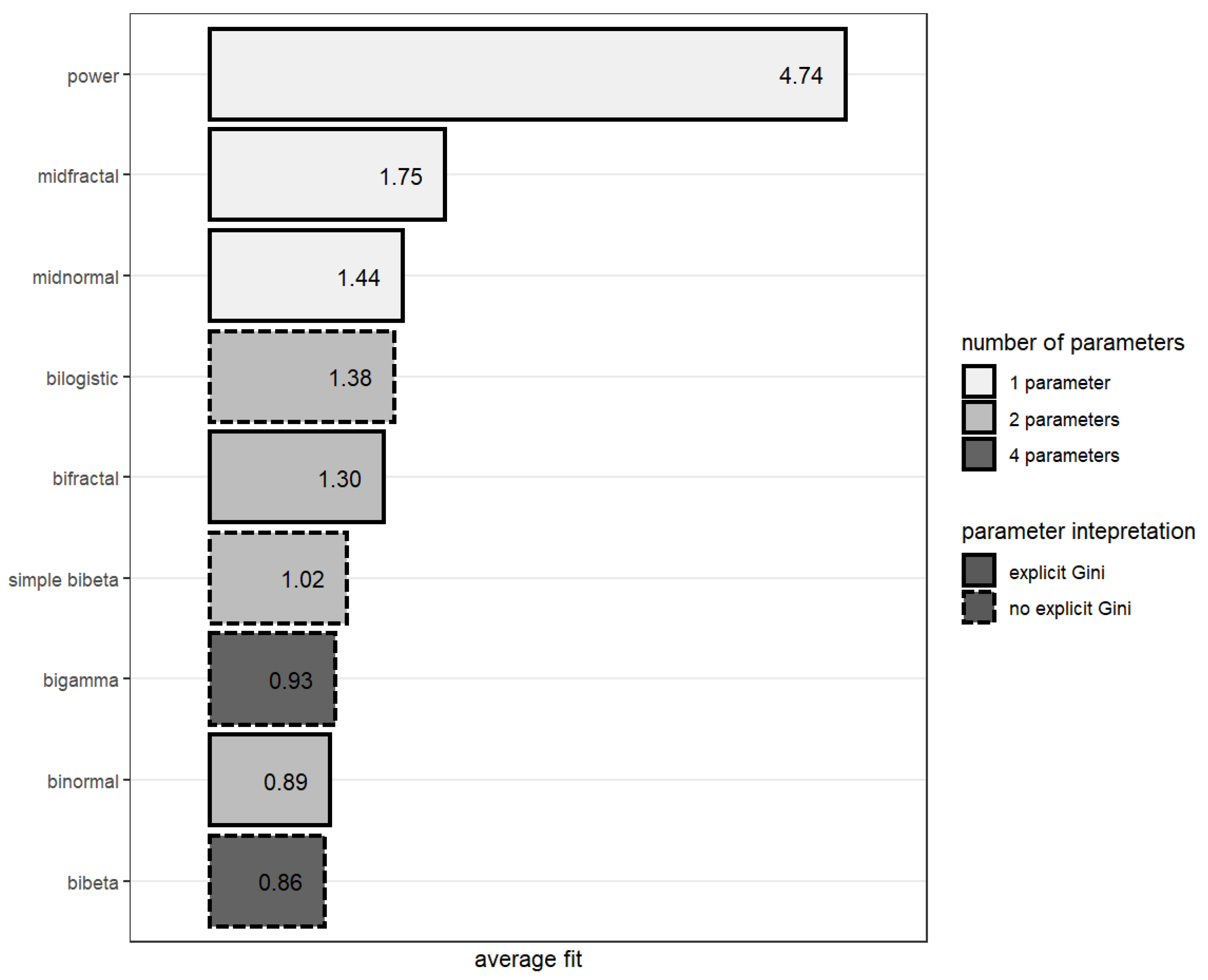
Figure 4 summarises findings from Table 2 and presents the average goodness of fit (square root of ) for each model. The summarised data showed that all the models presented, except for the power curve, were comparable in terms of the average goodness of fit. However, both four-parameter models (bibeta and bigamma) and the binormal model were, on average, the ones matching the data best.
5. Discussion and Conclusions
The empirical results presented in the previous section constitute the first—as far as we know—test of various ROC curve models against empirical credit-scoring data. They show that the bibeta model, on average, fits the empirical data best. The goodness of fit for the binormal model is at a comparable level. The binormal model is also the model that proved to be the best fit for the largest number of data sets. Obviously, the obtained results can be reinforced or undermined by further research based on more data on empirical ROC curves. This is one of the reasons why we are sharing the code used in this article that would allow anyone interested to perform such tests.
It is worth noting that ROC curve models are not predictive statistical models, as understood by, e.g., Hastie et al. (2016). ROC curve models are descriptive mathematical models; some are parametric (they use assumptions about probability distributions), whereas others are purely algebraic. Their primary purpose is to approximately describe empirical ROC curves. Therefore, the methods of selecting and assessing predictive models (Hastie et al. 2016; Ramspek et al. 2021) are not directly applicable in the exercise presented in the preceding section, as it is not about finding the best predictive model. Instead, it is an exercise in finding the best theoretical curve approximating the empirical one. It is somewhat similar to the curve-fitting tasks in computer science or engineering (Fang and Gossard 1995; Frisken 2008; Guest 2012). The minimum distance approach proposed and described by Hsieh and Turnbull (1996), Davidov and Nov (2012), and Jokiel-Rokita and Topolnicki (2019) seems to be the optimal method for such an exercise as it allows for fitting both parametric and algebraic curves in the same, unified way.
When assessing the appropriateness of a particular ROC curve model, not only the goodness of fit counts. One should consider some other aspects, including the number of parameters and the possibility of interpreting them. Intuitively, the fewer parameters in the formula, other things being equal, the better. As illustrated in Figure 4, there were three models with only one parameter (the Gini coefficient of a given scorecard): the midnormal, midfractal, and power models. The midnormal curve was the best-fitting model in this category. The binormal, bifractal, bilogistic and simple bibeta models require two parameters. The binormal model won over all the other two-parameter models. The best-fitting (on average) model, the bibeta curve, has four parameters.
From the perspective of the credit-scoring modelling practice, it is vital to have an explicit Gini/AUC parameter in the ROC formula (Kochański 2021). Models based on fractal curves (the bifractal and midfractal models) fulfil this postulate. When Equation (21) is the basis of a binormal (or midnormal) curve, the explicit Gini parameter is also available. A power curve is another example of a curve that can be defined so that its (one and only) parameter is the Gini coefficient. Still, as shown in the previous section, its fit with the empirical data was much worse than that of the competing models. In consequence, there were five models with an explicit Gini parameter on our list; other models did not allow for simple reformulation aimed at obtaining the Gini coefficient as the input.
The other parameter of the bifractal model, responsible for the shape of the curve, also has an apparent meaning. However, the bifractal model lacks a theoretical foundation, which may be considered a substantial disadvantage of this approach.
A potential shortcoming of the binormal model is the presence of “hooks”, i.e., nonconcave regions that are irrational for the ROC curve. Such a “hook” is a portion of the curve below the 45º diagonal, which makes random guessing in these regions a better option than making decisions based on the ROC. Curves with such “hooks” are referred to as “improper” curves. To address this shortcoming, “proper” ROC curves have been suggested (Chen and Hu 2016; Dorfman et al. 1997; Metz and Pan 1999).
It seems that in practice, in the credit-scoring context, the “improperness” does not constitute a problem. The binormal curve demonstrates no hooks for b = 1, and if b is close to 1, the size of the hook regions is negligible from a practical standpoint. For the empirical data sets from Section 3, the maximum b of the fitted binormal curve was 1.29, and the minimum was 0.79. Visual inspection confirmed that the hooks were not visible (yet they were present; for example, for the fitted binormal curve with b = 1.29 and γ = 0.74, there was a hook region for x < 10−9).
Another argument against the binormal/midnormal curves (as well as against the bibeta and bigamma) is that these models require quite complex mathematical operations (Birdsall 1973, pp. 100–8). Such an argument would support the bilogistic and bifractal model; however, thanks to the availability of specialised computer software and cheap computing power, it is not as important as it probably would have been half a century ago.
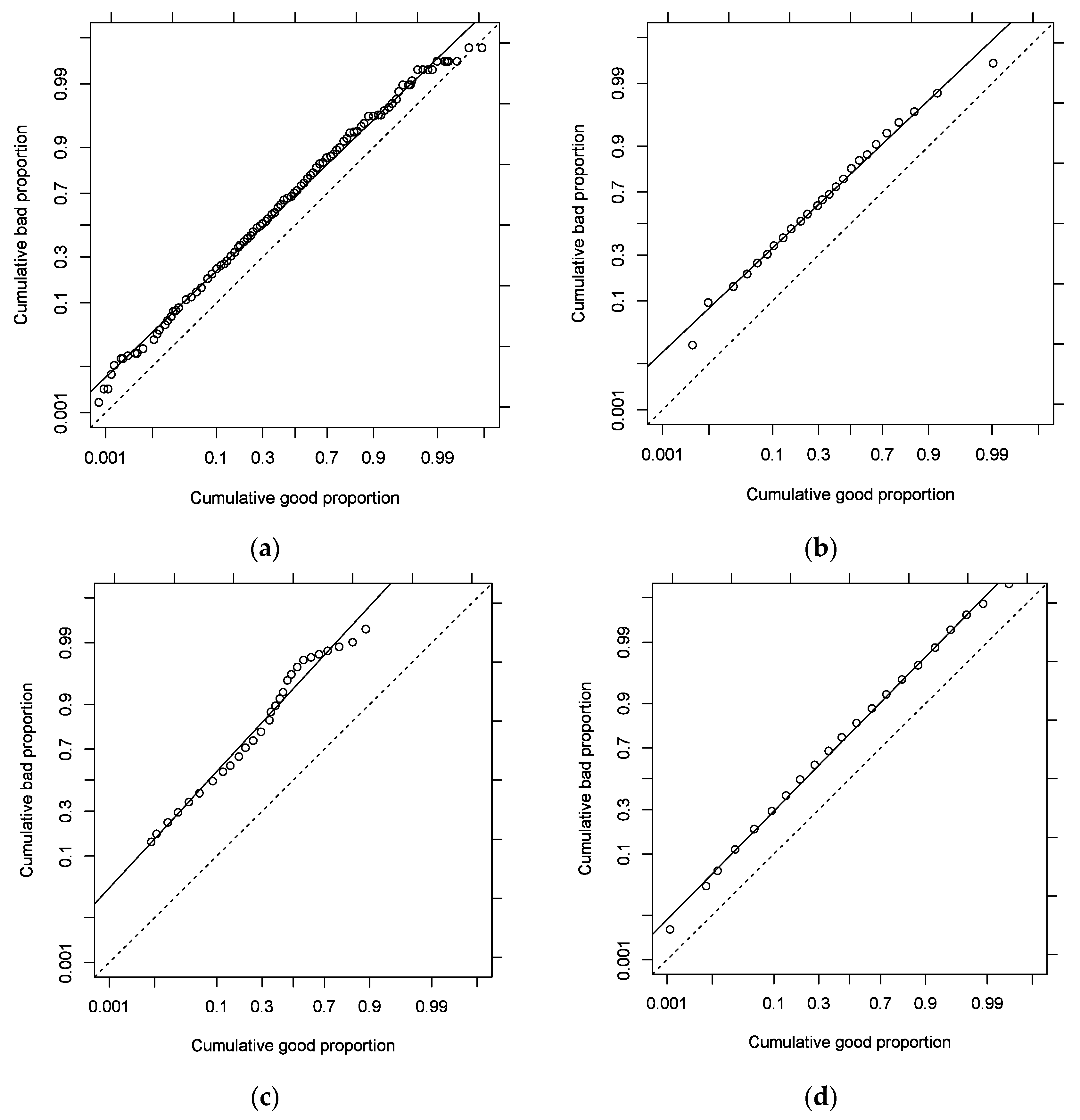
Hanley (1988) summarised the arguments in favour of the binormal model. The claims included mathematical tractability and convenience, and theoretical considerations. Empirical results (Swets 1986) have also shown that the model fits the data quite well. Additionally, as shown by Hanley (1988), because of the relative scarcity of medical data, the random noise is much more visible than the deviations driven by the differences between the models. The scarcity of data is a less frequent problem in the credit-scoring domain, but the empirical argument (the fit turns out to be the best for many real-life instances) is even more vital. Figure 5 shows the results of a visual inspection as proposed by Swets (1986). The plots are “binormal” in the sense that the cumulative bad and good proportions were rescaled according to their standard normal distribution deviates (Φ−1(x) and Φ−1(y)). If the binormal model is adequate, then the empirical data points should gather along a straight line. For most of the empirical curves presented Section 3, this was true. The data from Tobback and Martens (2019) had the most pronounced deviations (see the irregular shape in Figure 5c), but none of the other ROC curve models could explain this anomaly.
Table 3 brings together the advantages and disadvantages of the ROC curve models discussed in this article.
So far, the literature on the subject of credit scoring has not devoted much attention to ROC curve models. With the exception of Satchell and Xia (2008), Kürüm et al. (2012), and Kochański (2021), we did not find articles in this area that directly refer to curve models, binormal or others. This study helps to fill that gap and provides credit-risk managers and researchers with a useful set of ROC curve modelling tools. As demonstrated in the literature section, ROC curve models are valuable for credit-risk management. They provide methods for determining confidence intervals and inferring the AUROC from a sample. Thanks to them, it is possible to model the impact of scoring models that have not yet been built. They also allow for a concise description of the curve shape: a scorecard with the same AUROC but a different shape of the curve may be used differently (cutting off the worst customers versus selecting the best of the best). Each of these applications deserves separate research; the results provided in this paper provide a good starting point for such studies.
Concluding, the binormal model seems to be the optimal approach to modelling credit-scoring ROC curves. When a one-parameter ROC curve model is needed, the midnormal (the binormal model with equal variances assumption) seems to be the right choice. The binormal model can be accommodated to have the Gini coefficient as a parameter. This feature is quite essential from a credit-risk-management perspective. Additionally, the mathematical tractability of the model, as well as convenience and theoretical considerations provide arguments in favour of this approach. “Improperness” of the binormal model (presence of nonconcave “hook” regions if variances are not equal) seems to have little practical importance.
Funding
This research received no external funding.
Data Availability Statement
The data and R code performing the calculations as well as generating the graphs are made available in the script file roc_curves_fitting.R at https://github.com/roccurves/scoringROCcurves/blob/main/roc_curves_fitting.R.
Conflicts of Interest
The author declares no conflict of interest.
References
- Anderson, Raymond. 2007. The Credit Scoring Toolkit: Theory and Practice for Retail Credit Risk Management and Decision Automation. Oxford: Oxford University Press. [Google Scholar]
- Atapattu, Saman, Chintha Tellambura, and Hai Jiang. 2010. Analysis of area under the ROC curve of energy detection. IEEE Transactions on Wireless Communications 9: 1216–25. [Google Scholar] [CrossRef]
- Bamber, Donald. 1975. The area above the ordinal dominance graph and the area below the receiver operating characteristic graph. Journal of Mathematical Psychology 12: 387–415. [Google Scholar] [CrossRef]
- Bandos, Andriy I., Ben Guo, and David Gur. 2017. Estimating the Area Under ROC Curve When the Fitted Binormal Curves Demonstrate Improper Shape. Academic Radiology 24: 209–19. [Google Scholar] [CrossRef] [PubMed]
- Berg, Tobias, Valentin Burg, Ana Gombović, and Manju Puri. 2020. On the Rise of FinTechs: Credit Scoring Using Digital Footprints. The Review of Financial Studies 33: 2845–97. [Google Scholar] [CrossRef]
- Bewick, Viv, Liz Cheek, and Jonathan Ball. 2004. Statistics review 13: Receiver operating characteristic curves. Critical Care 8: 508. [Google Scholar] [CrossRef]
- Birdsall, Theodore G. 1973. The Theory of Signal Detectability: ROC Curves and Their Character. Ann Arbor: Cooley Electronics Laboratory, Department of Electrical and Computer Engineering, The University of Michigan. [Google Scholar]
- Blöchlinger, Andreas, and Markus Leippold. 2006. Economic benefit of powerful credit scoring. Journal of Banking & Finance 30: 851–73. [Google Scholar] [CrossRef]
- Bowyer, Kevin, Christine Kranenburg, and Sean Dougherty. 2001. Edge Detector Evaluation Using Empirical ROC Curves. Computer Vision and Image Understanding 84: 77–103. [Google Scholar] [CrossRef]
- Bradley, Andrew P. 1997. The use of the area under the ROC curve in the evaluation of machine learning algorithms. Pattern Recognition 30: 1145–59. [Google Scholar] [CrossRef]
- Chang, Chein-I. 2010. Multiparameter Receiver Operating Characteristic Analysis for Signal Detection and Classification. IEEE Sensors Journal 10: 423–42. [Google Scholar] [CrossRef]
- Chen, Weijie, and Nan Hu. 2016. Proper Bibeta ROC Model: Algorithm, Software, and Performance Evaluation. In Medical Imaging 2016: Image Perception, Observer Performance, and Technology Assessment. Presented at the Medical Imaging 2016: Image Perception, Observer Performance, and Technology Assessment, SPIE, San Diego, CA, USA, March 2; pp. 97–104. [Google Scholar] [CrossRef]
- Conolly, Stephen. 2017. Personality and Risk: A New Chapter for Credit Assessment. Presented at the Credit Scoring and Credit Control XV Conference, Edinburgh, UK, August 30–September 1; Available online: https://www.business-school.ed.ac.uk/crc-conference/accepted-papers (accessed on 27 April 2018).
- Cook, Nancy R. 2007. Use and misuse of the receiver operating characteristic curve in risk prediction. Circulation 115: 928–35. [Google Scholar] [CrossRef]
- Cook, Nancy R. 2008. Statistical evaluation of prognostic versus diagnostic models: Beyond the ROC curve. Clinical Chemistry 54: 17–23. [Google Scholar] [CrossRef] [PubMed]
- Davidov, Ori, and Yuval Nov. 2012. Improving an estimator of Hsieh and Turnbull for the binormal ROC curve. Journal of Statistical Planning and Inference 142: 872–77. [Google Scholar] [CrossRef]
- Djeundje, Viani B., Jonathan Crook, Raffaella Calabrese, and Mona Hamid. 2021. Enhancing credit scoring with alternative data. Expert Systems with Applications 163: 113766. [Google Scholar] [CrossRef]
- Dorfman, Donald D., Kevin S. Berbaum, Charles E. Metz, Russell V. Lenth, James A. Hanley, and Hatem Abu Dagga. 1997. Proper Receiver Operating Characteristic Analysis: The Bigamma Model. Academic Radiology 4: 138–49. [Google Scholar] [CrossRef]
- England, William L. 1988. An Exponential Model Used for Optimal Threshold Selection on ROC Curves. Medical Decision Making 8: 120–31. [Google Scholar] [CrossRef]
- Fang, Lian, and David C. Gossard. 1995. Multidimensional curve fitting to unorganized data points by nonlinear minimization. Computer-Aided Design 27: 48–58. [Google Scholar] [CrossRef]
- Faraggi, David, and Benjamin Reiser. 2002. Estimation of the area under the ROC curve. Statistics in Medicine 21: 3093–106. [Google Scholar] [CrossRef]
- Faraggi, David, Benjamin Reiser, and Enrique F. Schisterman. 2003. ROC curve analysis for biomarkers based on pooled assessments. Statistics in Medicine 22: 2515–27. [Google Scholar] [CrossRef]
- Fawcett, Tom. 2006. An Introduction to ROC Analysis. Pattern Recognition Letters 27: 861–74. [Google Scholar] [CrossRef]
- Frisken, Sarah F. 2008. Efficient Curve Fitting. Journal of Graphics Tools 13: 37–54. [Google Scholar] [CrossRef]
- Gneiting, Tilmann, and Peter Vogel. 2022. Receiver operating characteristic (ROC) curves: Equivalences, beta model, and minimum distance estimation. Machine Learning 111: 2147–59. [Google Scholar] [CrossRef]
- Gonçalves, Luzia, Ana Subtil, M. Rosário Oliveira, and Patricia de Zea Bermudez. 2014. ROC Curve Estimation: An Overview. REVSTAT-Statistical Journal 12: 1–20. [Google Scholar] [CrossRef]
- Gönen, Mithat, and Glenn Heller. 2010. Lehmann Family of ROC Curves. Medical Decision Making 30: 509–17. [Google Scholar] [CrossRef]
- Guest, Philip George. 2012. Numerical Methods of Curve Fitting. Cambridge: Cambridge University Press. [Google Scholar]
- Guido, Giuseppe, Sina Shaffiee Haghshenas, Sami Shaffiee Haghshenas, Alessandro Vitale, Vincenzo Gallelli, and Vittorio Astarita. 2020. Development of a Binary Classification Model to Assess Safety in Transportation Systems Using GMDH-Type Neural Network Algorithm. Sustainability 12: 6735. [Google Scholar] [CrossRef]
- Hahm, Joon-Ho, and Sangche Lee. 2011. Economic Effects of Positive Credit Information Sharing: The Case of Korea. Applied Economics 43: 4879–90. [Google Scholar] [CrossRef]
- Hajian-Tilaki, Karimollah. 2013. Receiver Operating Characteristic (ROC) Curve Analysis for Medical Diagnostic Test Evaluation. Caspian Journal of Internal Medicine 4: 627–35. [Google Scholar]
- Hamel, Lutz. 2009. Model Assessment with ROC Curves. In Encyclopedia of Data Warehousing and Mining, 2nd ed. Pennsylvania: IGI Global. [Google Scholar] [CrossRef]
- Hand, David J. 2009. Measuring classifier performance: A coherent alternative to the area under the ROC curve. Machine Learning 77: 103–23. [Google Scholar] [CrossRef]
- Hand, David J., and Christoforos Anagnostopoulos. 2013. When is the area under the receiver operating characteristic curve an appropriate measure of classifier performance? Pattern Recognition Letters 34: 492–95. [Google Scholar] [CrossRef]
- Hanley, James A. 1988. The Robustness of the “Binormal” Assumptions Used in Fitting ROC Curves. Medical Decision Making 8: 197–203. [Google Scholar] [CrossRef] [PubMed]
- Hanley, James A. 1996. The Use of the ‘Binormal’ Model for Parametric ROC Analysis of Quantitative Diagnostic Tests. Statistics in Medicine 15: 1575–85. [Google Scholar] [CrossRef]
- Hastie, Trevor, Robert Tibshirani, and Jerome Friedman. 2016. The Elements of Statistical Learning: Data Mining, Inference, and Prediction, 2nd ed. New York: Springer. [Google Scholar]
- Hautus, Michael J., Michael O’Mahony, and Hye-Seong Lee. 2008. Decision Strategies Determined from the Shape of the Same–Different ROC Curve: What Are the Effects of Incorrect Assumptions? Journal of Sensory Studies 23: 743–64. [Google Scholar] [CrossRef]
- Hsieh, Fushing, and Bruce W. Turnbull. 1996. Nonparametric and semiparametric estimation of the receiver operating characteristic curve. The Annals of Statistics 24: 25–40. [Google Scholar] [CrossRef]
- Idczak, Adam Piotr. 2019. Remarks on Statistical Measures for Assessing Quality of Scoring Models. Acta Universitatis Lodziensis. Folia Oeconomica 4: 21–38. [Google Scholar] [CrossRef]
- Iyer, Rajkamal, Asim Ijaz Khwaja, Erzo F. P. Luttmer, and Kelly Shue. 2016. Screening Peers Softly: Inferring the Quality of Small Borrowers. Management Science 62: 1554–77. [Google Scholar] [CrossRef]
- Janssens, A. Cecile J. W., and Forike K. Martens. 2020. Reflection on modern methods: Revisiting the area under the ROC Curve. International Journal of Epidemiology 49: 1397–403. [Google Scholar] [CrossRef]
- Jennings, Andrew. 2015. Expanding the Credit Eligible Population in the USA. Presented at the Credit Scoring and Credit Control XIV Conference—Conference Papers, Edinburgh, UK, August 26–28; Available online: https://www.business-school.ed.ac.uk/crc/category/conference-papers/2015/ (accessed on 27 April 2018).
- Jokiel-Rokita, Alicja, and Rafał Topolnicki. 2019. Minimum distance estimation of the binormal ROC curve. Statistical Papers 60: 2161–83. [Google Scholar] [CrossRef]
- Kochański, Błażej. 2021. Bifractal Receiver Operating Characteristic Curves: A Formula for Generating Receiver Operating Characteristic Curves in Credit-Scoring Contexts. Journal of Risk Model Validation 15: 1–18. [Google Scholar] [CrossRef]
- Krzanowski, Wojtek J., and David J. Hand. 2009. ROC Curves for Continuous Data, 1st ed. London: Chapman and Hall/CRC. [Google Scholar]
- Kürüm, Efsun, Kasirga Yildirak, and Gerhard-Wilhelm Weber. 2012. A classification problem of credit risk rating investigated and solved by optimisation of the ROC curve. Central European Journal of Operations Research 20: 529–57. [Google Scholar] [CrossRef]
- Lahiri, Kajal, and Liu Yang. 2018. Confidence Bands for ROC Curves With Serially Dependent Data. Journal of Business & Economic Statistics 36: 115–30. [Google Scholar] [CrossRef]
- Lappas, Pantelis Z., and Athanasios N. Yannacopoulos. 2021. A machine learning approach combining expert knowledge with genetic algorithms in feature selection for credit risk assessment. Applied Soft Computing 107: 107391. [Google Scholar] [CrossRef]
- Levy, Bernard C. 2008. Principles of Signal Detection and Parameter Estimation, 2008th ed. Berlin: Springer. [Google Scholar]
- Lloyd, Chris J. 2000. Fitting ROC Curves Using Non-linear Binomial Regression. Australian & New Zealand Journal of Statistics 42: 193–204. [Google Scholar] [CrossRef]
- Mandrekar, Jayawant N. 2010. Receiver Operating Characteristic Curve in Diagnostic Test Assessment. Journal of Thoracic Oncology 5: 1315–16. [Google Scholar] [CrossRef] [PubMed]
- Metz, Charles E. 1978. Basic principles of ROC analysis. Seminars in Nuclear Medicine 8: 283–98. [Google Scholar] [CrossRef]
- Metz, Charles E., and Xiaochuan Pan. 1999. “Proper” Binormal ROC Curves: Theory and Maximum-Likelihood Estimation. Journal of Mathematical Psychology 43: 1–33. [Google Scholar] [CrossRef]
- Mossman, Douglas, and Hongying Peng. 2016. Using Dual Beta Distributions to Create “Proper” ROC Curves Based on Rating Category Data. Medical Decision Making 36: 349–65. [Google Scholar] [CrossRef]
- Ogilvie, John C., and C. Douglas Creelman. 1968. Maximum-likelihood estimation of receiver operating characteristic curve parameters. Journal of Mathematical Psychology 5: 377–91. [Google Scholar] [CrossRef]
- Omar, Luma, and Ioannis Ivrissimtzis. 2019. Using theoretical ROC curves for analysing machine learning binary classifiers. Pattern Recognition Letters 128: 447–51. [Google Scholar] [CrossRef]
- Park, Seong Ho, Jin Mo Goo, and Chan-Hee Jo. 2004. Receiver Operating Characteristic (ROC) Curve: Practical Review for Radiologists. Korean Journal of Radiology 5: 11–18. [Google Scholar] [CrossRef]
- Pencina, Michael J., Ralph B. D’Agostino Sr., Ralph B. D’Agostino Jr., and Ramachandran S. Vasan. 2008. Evaluating the added predictive ability of a new marker: From area under the ROC curve to reclassification and beyond. Statistics in Medicine 27: 157–72, discussion 207–12. [Google Scholar] [CrossRef]
- Ramspek, Chava L., Kitty J. Jager, Friedo W. Dekker, Carmine Zoccali, and Merel van Diepen. 2021. External validation of prognostic models: What, why, how, when and where? Clinical Kidney Journal 14: 49–58. [Google Scholar] [CrossRef]
- Řezáč, Martin, and František Řezáč. 2011. How to Measure the Quality of Credit Scoring Models. Czech Journal of Economics and Finance (Finance a Úvěr) 61: 486–507. [Google Scholar]
- Řezáč, Martin, and Jan Koláček. 2012. Lift-Based Quality Indexes for Credit Scoring Models as an Alternative to Gini and KS. Journal of Statistics: Advances in Theory and Applications 7: 1–23. [Google Scholar]
- Satchell, Stephen, and Wei Xia. 2008. 8—Analytic models of the ROC Curve: Applications to credit rating model validation. In The Analytics of Risk Model Validation. Edited by George Christodoulakis and Stephen Satchell. Cambridge: Academic Press, pp. 113–33. [Google Scholar] [CrossRef]
- Scallan, Gerard. 2013. Why You Shouldn’t Use the Gini. ARCA Retail Credit Conference, Leura, Australia. Available online: https://www.scoreplus.com/assets/files/Whats-Wrong-with-Gini-why-you-shouldnt-use-it-ARCA-Retail-Credit-Conference-Nov-2013.pdf (accessed on 29 June 2022).
- Shen, Feng, Xingchao Zhao, Gang Kou, and Fawaz E. Alsaadi. 2021. A new deep learning ensemble credit risk evaluation model with an improved synthetic minority oversampling technique. Applied Soft Computing 98: 106852. [Google Scholar] [CrossRef]
- Siddiqi, Naeem. 2017. Intelligent Credit Scoring: Building and Implementing Better Credit Risk Scorecards. Hoboken: John Wiley & Sons. [Google Scholar]
- Somers, Robert H. 1962. A New Asymmetric Measure of Association for Ordinal Variables. American Sociological Review 27: 799–811. [Google Scholar] [CrossRef]
- Swets, John A. 1986. Form of Empirical ROCs in Discrimination and Diagnostic Tasks: Implications for Theory and Measurement of Performance. Psychological Bulletin 99: 181–98. [Google Scholar] [CrossRef]
- Swets, John A. 2014. Signal Detection Theory and ROC Analysis in Psychology and Diagnostics: Collected Papers. London: Psychology Press. [Google Scholar] [CrossRef]
- Tang, Tseng-Chung, and Li-chiu Chi. 2005. Predicting multilateral trade credit risks: Comparisons of Logit and Fuzzy Logic models using ROC curve analysis. Expert Systems with Applications 28: 547–56. [Google Scholar] [CrossRef]
- Thomas, Lyn C. 2009. Consumer Credit Models: Pricing, Profit and Portfolios. Oxford: Oxford University Press. [Google Scholar]
- Thomas, Lyn, Jonathan Crook, and David Edelman. 2017. Credit Scoring and Its Applications, 2nd ed. Philadelphia: Society for Industrial and Applied Mathematics. [Google Scholar] [CrossRef]
- Tobback, Ellen, and David Martens. 2019. Retail Credit Scoring Using Fine-Grained Payment Data. Journal of the Royal Statistical Society: Series A (Statistics in Society) 182: 1227–46. [Google Scholar] [CrossRef]
- Tripathi, Diwakar, Damodar R. Edla, Venkatanareshbabu Kuppili, and Annushree Bablani. 2020. Evolutionary Extreme Learning Machine with novel activation function for credit scoring. Engineering Applications of Artificial Intelligence 96: 103980. [Google Scholar] [CrossRef]
- Wichchukit, Sukanya, and Michael O’Mahony. 2010. A Transfer of Technology from Engineering: Use of ROC Curves from Signal Detection Theory to Investigate Information Processing in the Brain during Sensory Difference Testing. Journal of Food Science 75: R183–R193. [Google Scholar] [CrossRef] [PubMed]
- Wójcicki, Bartosz, and Grzegorz Migut. 2010. Wykorzystanie skoringu do przewidywania wyłudzeń kredytów w Invest-Banku. In Skoring w Zarządzaniu Ryzykiem. Kraków: Statsoft, pp. 47–57. [Google Scholar]
- Xia, Yufei, Junhao Zhao, Lingyun He, Yinguo Li, and Mengyi Niu. 2020. A novel tree-based dynamic heterogeneous ensemble method for credit scoring. Expert Systems with Applications 159: 113615. [Google Scholar] [CrossRef]
Figure 1.
Bifractal curves.

Figure 2.
Binormal curves.

Figure 3.
Results of the fitting of ROC models to the D1 data.

Figure 4.
Average goodness of fit () for particular models.

Figure 5.
Empirical ROC curves on binormal plots. (a) A1 model; (b) Data from Řezáč and Řezáč (2011); (c) Data from Tobback and Martens (2019); (d) C1 model.
Figure 5.
Empirical ROC curves on binormal plots. (a) A1 model; (b) Data from Řezáč and Řezáč (2011); (c) Data from Tobback and Martens (2019); (d) C1 model.


Table 1.
Results of the fitting of four ROC models to the D1 data.
| Model | Parameters | Fitting Objective (fobj) |
|---|---|---|
| Binormal (Equation (21)) | b = 0.9539; γ = 0.4290 | fobj = 8.09 × 10⁻⁵ |
| Bifractal (Equation (19)) | β = 0.4239; γ = 0.4298 | fobj = 8.40 × 10⁻⁵ |
| Bilogistic (Equation (12)) | α0 = 1.2884; α1 = 0.9279 | fobj = 3.31 × 10⁻⁴ |
| Power (Equations (16) or (17)) | θ = 0.4072 or γ = 0.4212 | fobj = 1.27 × 10⁻³ |
Table 2.
ROC model curve fitting—the goodness of fit ().
| Binormal | Midnormal | Bifractal | Midfractal | Bilogistic | Bibeta | Simplified Bibeta | Bigamma | Power | |
|---|---|---|---|---|---|---|---|---|---|
| Berg et al. (2020), Credit Bureau model | 0.79 | 1.40 | 1.14 | 1.58 | 0.53 | 0.80 | 1.07 | 0.80 | 2.75 |
| Berg et al. (2020), Digital Footprint model2 | 0.53 | 2.14 | 1.00 | 2.25 | 1.35 | 0.53 | 0.65 | 0.64 | 2.66 |
| Conolly (2017), curve I | 0.84 | 1.40 | 1.19 | 1.71 | 1.22 | 0.90 | 0.94 | 0.95 | 5.15 |
| Conolly (2017), curve II | 0.82 | 0.94 | 1.06 | 1.14 | 0.80 | 0.83 | 0.96 | 0.94 | 2.46 |
| Jennings (2015) | 0.75 | 1.09 | 1.38 | 1.64 | 0.78 | 0.77 | 1.11 | 0.80 | 5.76 |
| Hahm and Lee (2011), model A | 1.38 | 3.14 | 2.13 | 3.59 | 1.06 | 1.45 | 1.70 | 1.39 | 3.39 |
| Hahm and Lee (2011), model B | 0.68 | 0.95 | 1.65 | 1.79 | 1.11 | 0.91 | 1.04 | 0.69 | 5.24 |
| Iyer et al. (2016) | 0.42 | 1.42 | 1.04 | 1.77 | 1.29 | 0.43 | 0.61 | 0.42 | 6.13 |
| Řezáč and Řezáč (2011) | 0.82 | 1.11 | 1.34 | 1.58 | 1.11 | 0.90 | 1.05 | 1.05 | 5.21 |
| Řezáč and Řezáč (2011)—additional data points read from the graph | 0.53 | 0.53 | 0.71 | 0.72 | 1.50 | 0.50 | 0.53 | 0.52 | 4.45 |
| Tobback and Martens (2019) | 1.95 | 2.52 | 1.89 | 2.51 | 3.24 | 1.08 | 1.64 | 1.60 | 7.55 |
| Wójcicki and Migut (2010) | 0.67 | 0.98 | 1.66 | 1.80 | 1.63 | 0.68 | 0.85 | 0.74 | 6.54 |
| Model A1 | 0.50 | 0.55 | 0.68 | 0.73 | 0.88 | 0.51 | 0.62 | 0.60 | 3.36 |
| Model A2 | 0.68 | 0.81 | 0.80 | 0.88 | 0.88 | 0.68 | 0.80 | 0.78 | 3.00 |
| Model B1 | 0.90 | 0.90 | 1.34 | 1.40 | 2.04 | 0.82 | 0.83 | 0.84 | 5.41 |
| Model B2 | 1.66 | 3.32 | 1.69 | 3.32 | 1.55 | 1.67 | 1.81 | 1.83 | 8.61 |
| Model B3 | 1.71 | 2.27 | 2.08 | 2.63 | 2.61 | 1.55 | 1.60 | 1.57 | 4.03 |
| Model C1 | 0.46 | 0.71 | 0.95 | 1.13 | 0.72 | 0.49 | 0.79 | 0.78 | 4.78 |
| Model D1 | 0.90 | 1.18 | 0.92 | 1.13 | 1.82 | 0.78 | 0.79 | 0.79 | 3.57 |
Table 3.
ROC curve models—pros and cons.
| Model | Pros | Cons |
|---|---|---|
| Bigamma/bibeta/simple bibeta | Good fit. “Proper” with some restrictions. | 4 parameters (2 in case of simple bibeta), no explicit AUROC parameter, complicated implementation (requires beta and gamma distribution functions). |
| Bilogistic | 2 parameters, simple mathematical operations. | On average, the worst among the models with more than one parameter, presence of non-concave regions. |
| Bifractal/midfractal | 2 parameters (or 1 in case of midfractal), explicit Gini parameter, interpretable shape parameter, only the simplest mathematical operations needed, monotone in the whole domain. | Lack of theoretical background, clearly “algebraic”. |
| Binormal/midnormal | 2 parameters (or 1 in case of midnormal), the model may be reformulated to produce an explicit Gini parameter. Mathematical tractability, convenience, good empirical fit in case of credit scoring and in other domains. | Presence of “hooks”: non-concave regions of the curve if b ≠ 1. |
| Power | One parameter | Very poor fit. |
Publisher’s Note: MDPI stays neutral with regard to jurisdictional claims in published maps and institutional affiliations. |
© 2022 by the author. Licensee MDPI, Basel, Switzerland. This article is an open access article distributed under the terms and conditions of the Creative Commons Attribution (CC BY) license (https://creativecommons.org/licenses/by/4.0/).
Share and Cite
MDPI and ACS Style
Kochański, B. Which Curve Fits Best: Fitting ROC Curve Models to Empirical Credit-Scoring Data. Risks 2022, 10, 184. https://doi.org/10.3390/risks10100184
AMA Style
Kochański B. Which Curve Fits Best: Fitting ROC Curve Models to Empirical Credit-Scoring Data. Risks. 2022; 10(10):184. https://doi.org/10.3390/risks10100184
Chicago/Turabian StyleKochański, Błażej. 2022. "Which Curve Fits Best: Fitting ROC Curve Models to Empirical Credit-Scoring Data" Risks 10, no. 10: 184. https://doi.org/10.3390/risks10100184
Note that from the first issue of 2016, this journal uses article numbers instead of page numbers. See further details here.