Growth of Defect-Induced Carbon Nanotubes for Low-Temperature Fruit Monitoring Sensor

Abstract

Herein, a carbon nanotubes-based sensor has been grown for the purpose of ethylene detection. The prepared CNTs had a crystalline structure with a smooth surface of 11.0 nm in diameter and 10.0 µm in length. The low-intensity graphite peak (G-band) as compared to the peak of the defect (D-band) characterizes the defects in the CNTs. An MWNTs-gas sensor was fabricated for monitoring the ethylene gas. The highest response was recorded at a low operating temperature of 30 °C. The sensor was also examined at 300 ppb up to 10 ppm and it showed a response of 2% up to 28%. The sensor response and recovery time constants were varied from 60 to 300 s, depending on the gas concentration. The results that were obtained for the synthetic ethylene gas were also compared with the real measurements for banana ripening. The results confirmed that the sensor is appropriate for the monitoring of fruit ripening.

1. Introduction

Avoiding food spoilage, such as that seen in fruits and vegetables, is the strategy of the commercial market. The fruits and vegetables are running quickly toward ripeness if they are exposed to more ethylene gas. Thus, the people responsible for transporting the product want to know how the product situation is going, and whether they need to take any action to keep it in a safe condition. For example, the condition of the fruit in various distribution chains is controlled by monitoring the ethylene level at every stage of the journey. The level of ethylene gas that is emitted from the products should be controlled when managing long-term storage.

Ethylene gas is an unsaturated hydrocarbon and a very important plant hormone. Ethylene gas emissions from the fruits during ripeness are sweet-smelling and colorless [1]. The emission of ethylene affects the aging and ripeness of adjacent fruits [2,3]. Although ethylene is useful in accelerating the ripening of fruits, it is harmful and causes food spoilage in some cases [4,5].

Few reports are available for the gas adsorption of ethylene as a detector for fruit ripening [6,7,8,9,10,11,12,13]. However, reaching cost-effective, simple, and good performance remains challenging. Gas-chromatographs [7], optical [10,11], and acoustic waves [12], which are expensive techniques, are currently used to detect ethylene gas. The electrochemical [13] and chemo-resistive [14,15] sensors are also studied. The conductometric/chemical-resistor sensors are simple, and they have the advantage of integrating into the micro-sensing device.

CNTs chemiresistor sensors have been widely studied due to their sensitivity to many gases, operation at room temperature, and extremely low detection advantage [8,16,17,18,19]. So far, there are open questions regarding the basic mechanism of CNTs sensing. It is known that the main gas sensing mechanism for a sensor that is composed of carbon nanotubes depends on the change in the concentration of the charge carriers in the nanotubes. There are two possible mechanisms: the variations of Schottky barriers at the contact points between the carbon nanotubes and metal electrodes, and the charge transfer due to the adsorption of gas molecules onto the carbon nanotubes surface.

A study was carried out for a device that was made of a single carbon nanotube connected by metal electrodes. The electrodes were covered with a protective layer, where most of the surface of the carbon nanotube was exposed. This study has provided evidence that the Schottky barrier variation is the main detection mechanism for gas sensing [20,21]. However, when experiments were performed on carbon nanotube networks, the situation became less clear, which suggests that the adsorption of gas molecules onto carbon nanotubes was primarily responsible for the conductivity change [22]. Additionally, there has been a theoretical study done on NO₂ through the density functional theory (DFT). This study demonstrated that NO₂ is absorbed on the tube surfaces within the network. However, subsequent work concluded that NO₂ binds more strongly to the interstitial regions between tubes. Thus, the molecules preferentially interact with more carbon nanotubes [23,24]. Moreover, the gas adsorption can be affected by the defects in the tubes or local functionalization of the CNT wall, where these defects sites can provide additional places for molecular bonding [25]. Therefore, the MWNTs are a promising candidate for obtaining more induced defects and additional interstitial regions. Hence, they are suitable for obtaining a good sensitivity and better performance towards gas molecules.

In this work, a sensing device was designed based on defect-induced CNTs that were synthesized by the PE-CVD technique for ethylene detection at low operating temperatures and very low gas concentrations. Raman spectroscopy and FESEM microscopy characterized the CNTs. The effect of working temperature on the sensor response under exposure to synthetic ethylene gas was also presented. The sensor was also tested at different ethylene concentrations to demonstrate the calibration curve and sensor ability in detecting a wide range of gas concentrations (300 ppb to 10 ppm). The sensor was investigated under a real condition for monitoring ethylene gas, which banana fruits produce during natural ripening.

2. Materials and Methods

Figure 1 illustrates the steps for the synthesis of the CNTs and the gas sensing device. The CNTs were grown on the Si/SiO₂ substrate. At first, the substrate was cleaned by deionized water, followed by ethanol, and drying in air. The substrate was coated with a Cr layer of ~5 nm and followed by a Ni catalyst layer of 18 nm, which was deposited using DC-sputtering. The substrate was then processed to grow CNTs by the PECVD method. The growth of CNTs was carried out using the system of the first-nano PECVD (3000-EasyTube-model). The carbon product obtained was carefully scratched for application in the characterization and sensing investigation.

The CNTs morphology was analyzed by using FE-SEM of Model JEOL JMS-7600F with low and high magnifications. The structure of CNTs was analyzed by confocal Raman microscope (LabRAM HR800) at room temperature and an ambient atmosphere with a He-Ne wavelength laser of 633 nm and power of 20 mW.

For fabricating the sensing device, two gold electrodes of ~200 µm were deposited on a glass substrate using DC sputtering, which was followed by scratched CNTs deposition (suspension in ethanol). Before the measurement, the sensor was dried at 60 °C for 30 min. in ambient air. The sensor was then tested using the gas sensing measurements system of model GSM-6000A. The system contains MFCs and a temperature-controlled Linkam chamber of model Linkam HFS600E-PB4 probe with a thermal stage of temperature accuracy of 0.1 °C, as shown in Figure 2. For examining the sensing performance, the sensor resistance was attained for the baseline in the airflow. The ethylene was passing in the sensing chamber with dry air at a flow rate of 200 mL/min. with a pressure of 1.0 atom. To keep the signal style, the sensor was exposed to the gas for ~200 s and then left to recover to the baseline for ~ 200 s. However, in some cases, the sensor may need more time to reach equilibrium. The measurements were performed using data acquisition (Keithley-2010, SweepMe 1.5.5 software). The sensing measurements were then carried out at various working temperatures that started from 30 °C up to 100 °C.

3. Results and Discussions

3.1. Morphology and Structure of CNTs

The morphology and structure of CNTs were expressed through scanning electron microscopy (SEM) and transmission electron microscopy (TEM), as shown in Figure 3. The FESEM images were observed for two high magnifications of 80,000 and 220,000, where CNTs morphology was described as a porous-like structure, as shown in Figure 3a,b. These porous CNTs are curvy, lengthy, and present interstitial contacts. The observed length and diameter of CNTs were about ~10 µm and ~11.0 nm, respectively. The diameter of the CNTs demonstrated that the CNT is combined with multilayers (MWNTS). The microstructure and materials morphology has numerous effects on the gas adsorption/desorption process onto the surface of the sensing layer. Thus, the curvy, lengthy, and porous structure is the most suitable for sensing performance. This type of structure has more surface defects, which work as active sites for gas molecules. Figure 3c,d present the relevant TEM images, which show that CNTs are multi-walled nanotubes and the diameter of the synthesized MWCNT was about 10–12 nm.

Raman analysis provides important information regarding the structure throughout the degree of crystallinity and disordering of the fabricated materials. The Raman spectrum qualitatively observed the defects inside the CNTs. The Raman spectrum of the fabricated CNTs was measured in the wavenumber range of 100–2800 cm⁻¹ through a He-Ne laser of 633 nm, as shown in Figure 4. Three modes were detected in the Raman spectrum, in which the peaks were assigned to D-, G-, and G’-bands corresponding to 1330, 1595, and 1645 cm⁻¹, respectively [26]. The intensity of the D-band was ascribed to the high defective points, where the ratio in the intensity of D/G peaks is approximately 2.1, which refers to defect-induced CNTs [27]. The observed bands describe the stretching vibrations of C-C bonds. The G-band is ascribed to the in-plane bond of stretching motion of Sp² pairs hybridized carbons and assigned to the symmetry of E_2g. The D-band describes the breathing mode of A_1g symmetry due to the disordering [28]. The G’-band provides information regarding the different interactions of the graphite interlayers in the depth of CNTs. The intensity ratio of G’- to G-band (G’/G = 0.17) indicates the multilayer formation of CNTs [29,30,31].

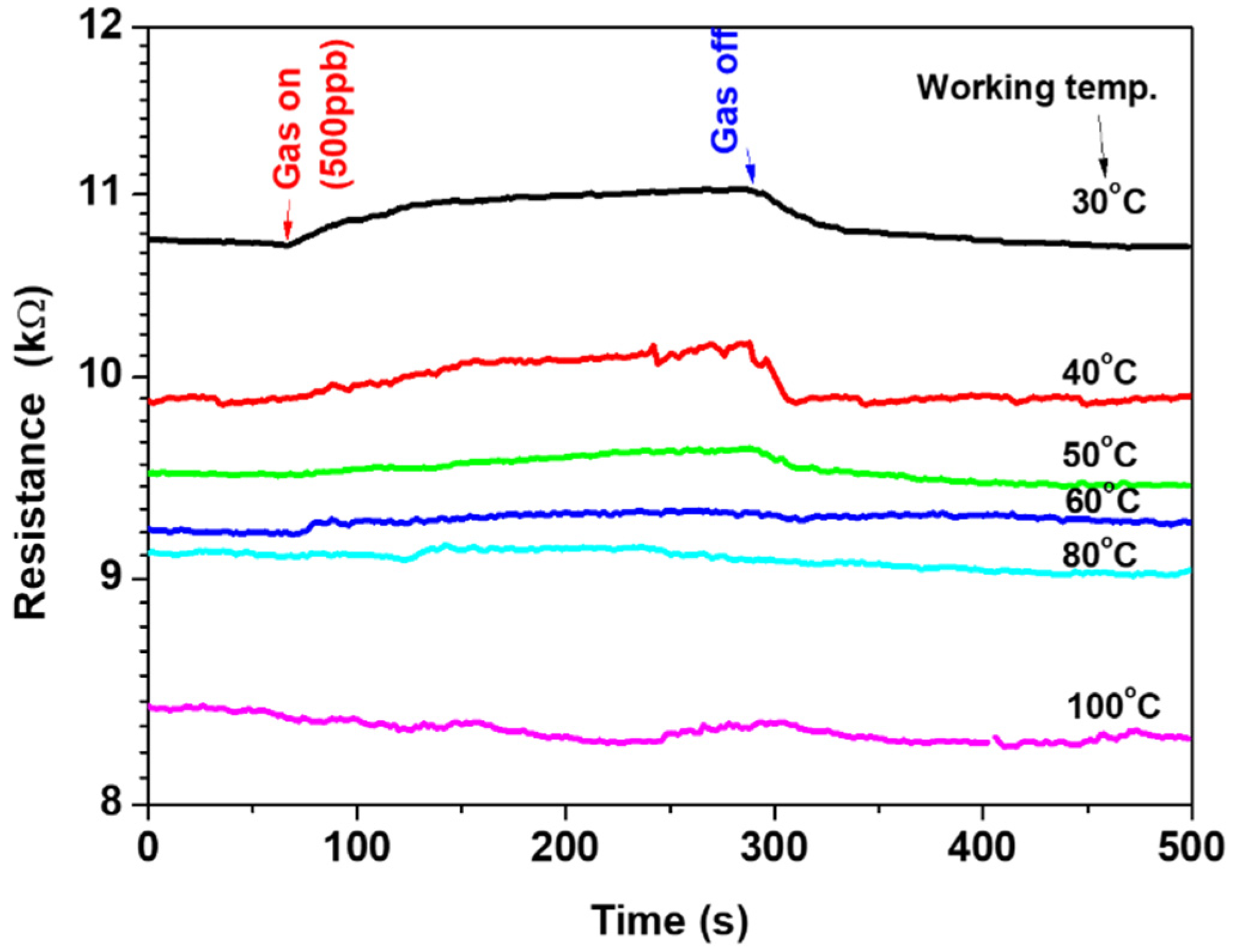
3.2. Sensor Response towards Ethylene Gas at Various Temperatures

The fabricated sensor was tested on 500-ppb-ethylene gas at various operating temperatures to define the most sensitive temperature. The operation/working temperature was varied from 30 °C up to 100 °C. Figure 5 shows the one-cycle signal of the sensor at various operating temperatures. The signal exhibited the effect of the gas on the electrical resistance of the sensor. The resistance increased upon exposure to the gas and then decreased when the gas flow was switched off. The signal is strong at a low temperature of 30 °C; however, it is weak at a high temperature of 80 °C, indicating the influence of the operating temperature on the sensor outputs. The electrical resistance decreased due to the increase in the operating temperature, showing semiconductor-like behavior. The selectivity of operation temperature confirmed the ability of the sensor to work at a low temperature of 30 °C.

Figure 6 calculates and depicts the sensor response based on the sensor outputs presented above. The sensor response (sensitivity, S) is defined as:

$$S\%=\frac{R_g-R_a}{R_a}\times 100$$

(1)

where R_a and R_g are the sensor resistances in air and air including gas, respectively. The response/sensitivity calculated at 30 °C is about 3%, corresponding to a low gas concentration of 500 ppb. This response gradually decreased to 2.8, 1.5, 1.0, 0.7, and 0.0% with increasing the working temperature to 40, 50, 60, 70, 80, and 100 °C, respectively. The empirical equation (S% = 4.88 − 0.062 T, where T in Celsius (°C)) formulated this decrease in the sensor response. The reduction in the sensor response at high temperatures may be explained in light of the results that were observed by Albesa et al. for the adsorption isothermal for ethylene on the CNTs [32]. In their study, the adsorption isotherms for ethylene on homogeneous nanotube were studied at 153, 273, and 343 K. They observed that the initial adsorption started at very low pressures and occurred on the interior sites of the CNTs. They found that, at 153 K, the adsorption curve displayed a sub-step at an average number of adsorbed molecules of 200. It was ascribed to the achievement of the first layer of ethylene molecules on the outer surface of CNTs. They also studied the effect of temperature on the simulated isotherms for ethylene that corresponds to the subsequent filling of the adsorption sites. The results concluded that, for all three temperatures, the density of the adsorbed phase in the internal sites of CNTs remained the same, while it was not the situation for the external sites. A disorder was observed for a gas molecule layer at the exterior surface of CNTs and it increased at high temperatures. Thus, their results are in agreement with the present sensing data, where it is expected that the adsorption of ethylene molecules will be much less at high temperatures.

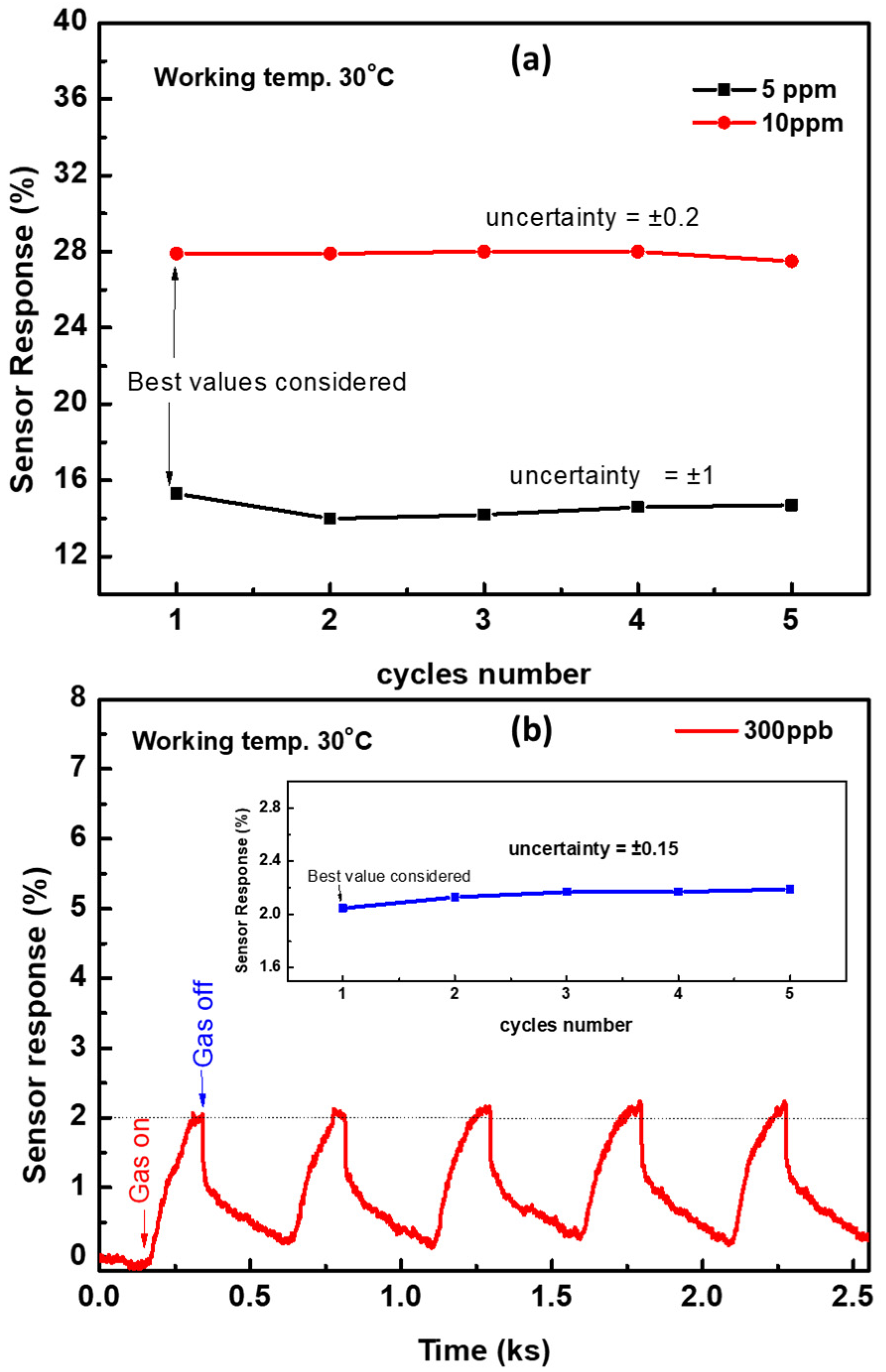
3.3. Sensor Response towards Ethylene Gas at Various Concentrations

The sensor was also investigated at various gas concentrations to understand its performance and demonstrate the calibration curve. This study was carried out at the most sensitive temperature of 30 °C. Figure 7 shows the resistance change (ΔR) of the device versus time as a function of gas concentration. The signal was recorded at the various gas concentrations of 300, 500, 1000, and 2000 ppb in sequence. The sensor signals increased with an increase of the gas concentration and exhibited a quick response/recovery towards the gas on/off.

For further investigations, the sensor was tested towards higher gas concentrations of 5.0 and 10.0 ppm at 30 °C. The signal was repeated five times to achieve the reversibility and repeatability of the sensor signals. The cycle time of the signal at these two concentrations is approximately 500 s (we give more time for the recovery time), as shown in Figure 8. The sensor outputs confirmed the repeatability and reversibility of the sensor signals. Based on the results that are observed in Figure 7 and Figure 8, the calibration curve was demonstrated, as shown in Figure 9. The calibration curve showed the ability of the sensor to respond and distinguish the change in gas concentration. However, two regions were observed for this curve; the first region is from 0.3 ppm up to 2.0 ppm, and the second is from 2.0 ppm up to 10 ppm. Both of the regions were proposed by a straight line with slopes of ~5.18 and ~2.17, respectively. The first region was ascribed to the high response towards the low gas concentrations. It may be due to the limitation of the active sites. The surface-active sites play an important role in sensor response.

The response and recovery time constants are very important parameters for describing the features of the sensor. These constants are defined as the time taken for resistance to reach 90% of its equilibrium (response/recovery), as demonstrated in the inset of Figure 10. The response and recovery times are calculated as a function of the gas concentration for the signal that is reported in Figure 7 and Figure 8. The response time constant (black mark) is about 60 s at a gas concentration of 0.3 ppm and it increased up to ~110 s at 10 ppm, as plotted in Figure 10. The recovery time constant (red mark) is ~120 s at a low concertation of 0.3 ppm and it increased linearly with an increasing the gas concentration. The response and recovery of the sensor are fast and reasonable.

The uncertainty/accuracy in the sensor response was calculated from the cyclic signals. The sensor response was measured at various cycles at gas concentrations of 5 and 10 ppm, as shown in Figure 8. Figure 11b clarifies the repeated signal at a low gas concentration of 300 ppb and the sensor response as a function of cycle number (inset) at this concentration. The sensor response is calculated as a function of the cycle number for 0.3, 5.0, and 10.0 ppm, as shown in Figure 11. Because there is no standard to measure uncertainty, we consider the first value of the response as the reference value, and then the change in the sensor response was calibrated to this value. We found that the uncertainty depends on the gas concentration. The best values of the sensor responses that were considered for 0.3, 5.0, and 10.0 ppm were 2.0, 15.3, and 27.9, respectively. The uncertainty was ±0.15, ±1.0, and ±0.2 for gas concentrations of 0.3, 5.0, and 10.0 ppm, which corresponded to exact percentage errors of 7.5, 6.5, and 0.7%, respectively. It seems that, at low concentrations, the uncertainty or error percentage, as compared to the sensor response, is higher than that of high concentrations. The reason is not well understood. However, we can assume that, at low gas concentrations, the gas molecules may not fill all active sites of the surface and they may adsorb on different sites at every cycle. Therefore, the response is not coming from the same active sites for every cycle. At high gas concentrations, the ethylene molecules might achieve a complete layer on the surface and the gas molecules fill most of the active sites, which results in a more stable sensor signal for every cycle.

3.4. Sensor Performance toward Various Gases and Humidity Conditions

Various gases, such as NO₂, NO, ethanol, acetone, and ethylene, were tested at the same working temperature of 30 °C to facilitate the comparison, and even the concentration was higher than ethylene concentration. The histogram of Figure 12 and its inset show the sensor signal and sensor response toward these gases. The sensor responds to these target gases, but with a different level of performance. The sensor signal shown in the inset exhibited that the sensor response and recovery of ethanol and acetone gases are faster than that of NO₂ and NO gases. The response to these gases has been calculated and compared, showing that the CNTs sensor is more sensitive for ethylene gas. It can be concluded that the CNTs-based sensor has good selectivity toward ethylene gas. The highest responses are found for ethylene, while the other gases show lower response values, as shown in Figure 12.

The effect of humidity on the performance of the fabricated gas sensor is applied by subjecting it to different humidity levels using a controlled humidity chamber (Humidity Series, Sheldon Manufacturing, Inc.). Figure 13 presents the effect of humidity conditions on the resistance of the fabricated sensor. Upon exposure to the humidity, the sensor resistance did not change until 50% humidity; however, it slightly increased with higher humidity. It was found that the maximum relative resistance change at 80% RH is about 0.02, which can be neglected. The results confirm that the present sensor can work well at various levels of humidity conditions.

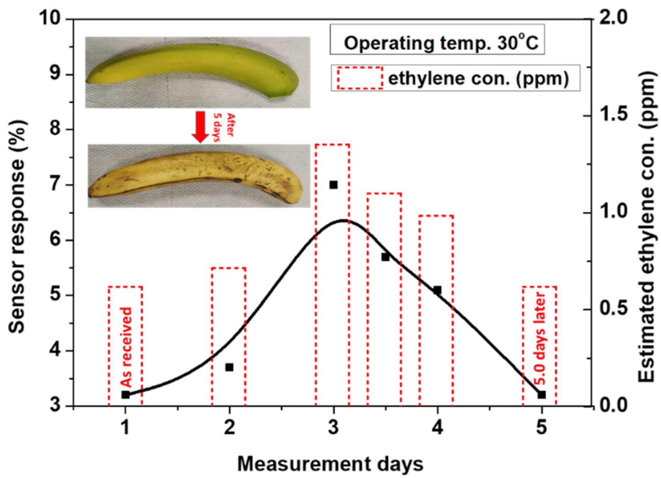
3.5. Sensor Response in a Real Condition

The device was tested to monitor the natural ripening of banana fruits in order to investigate the ability of the present sensor for monitoring the fruit quality. Xiao et al. reported a considerable study of ripeness controls by the ethylene production of natural ripeness of banana, 1-MCP-delayed, and ethylene-induced ripening [1]. They observed that the produced ethylene in natural ripening increased significantly after the 15th day of banana storage, attained the maximum level on day 18, and it then gradually reduced. Based on Xiao’s study, we have used a similar strategy as a guide for testing our device with banana natural ripening with ethylene production. Thus, a green-yellowish banana was brought as fresh fruit from the market. The ripeness of the banana over five days was detected by monitoring its produced ethylene. The measurements were carried out by placing the banana inside the glass jar, and then the synthetic air was flow at 200 SCCM through the jar to the sensing measurement chamber. The elapsed time from placing the banana to flow the air through the jar was approximately 5 min. to collect more gas from the banana. Figure 14 shows the estimated sensor response of the present device as a function of the ripening days at a working temperature of 30 °C. The sensor response of the green banana is about 2.8% on the first day of measurement. This response increased up to 7% on the third day, where the banana becomes mostly yellowish, and the ethylene emits at its highest level. With continued measurement for the fourth and fifth day, the dark spots started to cover the banana, and the sensor response decreases to the level of the first day. According to the data that were obtained in Figure 9, the equivalent ethylene concentration that is deduced from the sensor response during the banana ripening measurement can be estimated by the equation obtained from the first fitting line (S% = 5.18% C, where C is the gas concentration in ppm). The estimated ethylene concentration is presented as a histogram of the right side of Figure 14. These results are in agreement with the results presented by Xiao, confirming the ability of the present sensor to be integrated as a device for monitoring food quality.

We also performed cycling on a CNTs-based sensor to investigate the repeatability of the fabricated sensor, as shown in Figure 15. Figure 15a shows the response changes of the CNTs-based sensor as a function of time when the sensor was exposed to five cycles of a sequence of air, including produced ethylene (response for 180 s) and dry air (recovery for 300 s), according to three bananas with a different level of ripening, as shown in Figure 15b. It was found that the sensor has a good sensing performance during the sensing cycles without sensing decay, which suggests that the sensing characteristics were repeatable. Moreover, it is sensitive to various levels of banana ripening.

3.6. Sensing Mechanism toward Ethylene

The elucidation of the sensing mechanism of gas sensors based on CNTs remains challenging. In the present study, we attempt to propose a sensing mechanism that considers the intra-CNT mechanisms, which are modes of interaction between the analyte and CNTs. They include changes in the number or mobility of charge carriers and the generation of defects on the walls of CNTs. Charge transfer that is directly or indirectly induced by gas interactions will modulate the conductance of the CNTs by changing the concentration of the majority charge carriers. Because CNTs are p-doped, the exposure to further oxidizing gas will increase the hole conduction and cause a decrease in the resistance, while reducing gas will induce the reverse effect. The resistance increased when the ethylene molecules were introduced to the CNTs sensing layer, which suggested that more electrons are injected into the CNTs, where ethylene is bound with the CNTs at the interstitial or defect points, as shown in Figure 16. The direct charge transfer between the analyte and CNTs has been identified as a major sensing mechanism [33].

In the contact mechanism, the electrons are transferred between the Au electrode terminals to the CNT. The Fermi level of both materials reaches equilibrium where the Au Fermi level approaches the lowest unoccupied molecular orbital (LUMO) of the CNT [17,18]_. The ethylene molecules that accessed the sensor may bind with the electrode contacts, which decreases the carriers transport between the CNTs and Au electrode. However, we expect that the possibility of this mechanism contributing to the sensor conductivity is low when compared to the direct reaction with CNTs due to the large surface of CNTs, which are linked in a gap of 200 µm between electrodes. It is expected that there are large interstitials and defective sites in the sensing layer when compared to the electrode area. In other words, the mechanism of the Schottky barrier at the Au-contacts might be ignored here.

4. Conclusions

In summary, the CNTs were fabricated by plasma-enhanced chemical vapor deposition (PE-CVD), where the Si/SiO₂ substrate was coated by the Cr layer, followed by the Ni layer as catalysts. CNTs were indexed as defect-induced MWNTs with a high intensity of D-band when compared to the graphitic G-band. The morphology of CNTs exhibited features, such as a length of 10 µm and diameter of 11.0 nm. CNTs fabricated the gas sensing device, and it was applied for investigating the detection of ethylene gas at various temperatures and gas concentrations. The sensor showed a high response towards the low concentrations of ethylene gas. The maximum response recorded is approximately 7% at a temperature of 30 °C and gas concentration of 500 ppb. This response considerably increased up to ~29% when the gas concentration increased to 10 ppm. However, the sensor becomes less sensitive at high temperatures and insensitive at 100 °C. The present results show the capability of the defect-induced CNTs sensor. The response and recovery time constants were found to increase with the gas concentration with the reasonable values of 60–300 s at 0.3–10 ppm. The uncertainty in the sensor response is approximately ±0.15, ±1.0, and ±0.2 for 0.3, 5.0, and 10 ppm, corresponding to exact percentage errors of 7.5, 6.5, and 0.7%, respectively. Moreover, the device was tested in real conditions. The ability of the present sensor to monitor the fruit quality was investigated for monitoring the natural ripening of banana fruits. The sensor showed a good sensing performance during the sensing cycles without sensing decay, which suggests that the sensing characteristics were repeatable. The sensor that has been presented here demonstrated its ability to work well in food quality monitoring.

References

1. Xiao, Y.Y.; Kuang, J.F.; Qi, X.N.; Ye, Y.J.; Wu, Z.X.; Chen, J.Y.; Lu, W.J. A comprehensive investigation of starch degradation process and identification of a transcriptional activator MabHLH6 during banana fruit ripening. Plant Biotechnol. J. 2018, 16, 151–164. [Google Scholar] [CrossRef] [Green Version]
2. Kevany, B.M.; Tieman, D.M.; Taylor, M.G.; Cin, V.D.; Klee, H.J. Ethylene receptor degradation controls the timing of ripening in tomato fruit. Plant J. 2007, 51, 458–467. [Google Scholar] [CrossRef]
3. Nath, P.; Trivedi, P.K.; Sane, V.A.; Sane, A.P. Role of ethylene in fruit ripening. Ethyl. Action Plants. 2006, 151–184. [Google Scholar] [CrossRef]
4. Dhillon, W.S.; Mahajan, B.V.C. Ethylene and ethephon induced fruit ripening in pear. J. Stored Prod. Postharvest Res. 2011, 2, 45–51. [Google Scholar]
5. Mahajan, B.V.C.; Tajender, K.; Gill, M.I.S.; Dhaliwal, H.S.; Ghuman, B.S.; Chahil, B.S. Studies on optimization of ripening techniques for banana. J. Food Sci. Technol. 2010, 47, 315–319. [Google Scholar] [CrossRef] [PubMed] [Green Version]
6. Fong, D.; Luo, S.X.; Andre, R.S.; Swager, T.M. Trace Ethylene Sensing via Wacker Oxidation. ACS Cent. Sci. 2020, 6, 507–512. [Google Scholar] [CrossRef] [PubMed] [Green Version]
7. Sklorz, A.; Miyashita, N.; Schäfer, A.; Lang, W. Low level ethylene detection using preconcentrator/sensor combinations. Proc. IEEE Sens. 2010, 2494–2499. [Google Scholar] [CrossRef]
8. Popa, C.; Dumitras, D.C.; Patachia, M.; Banita, S. Improvement of a photoacoustic technique for the analysis of non-organic bananas during ripening process. Rom. J. Phys. 2015, 60, 1132–1138. [Google Scholar]
9. Li, J.; Du, Z.; Zhang, Z.; Song, L.; Guo, Q. Hollow waveguide-enhanced mid-infrared sensor for fast and sensitive ethylene detection. Sens. Rev. 2017, 37, 82–87. [Google Scholar] [CrossRef]
10. Chiang, M.C.; Hao, H.C.; Hsiao, C.Y.; Liu, S.C.; Yang, C.M.; Tang, K.T.; Yao, D.J. Gas sensor array based on surface acoustic wave devices for rapid multi-detection. In Proceedings of the 2012 IEEE Nanotechnology Materials and Devices Conference (NMDC2012), Waikiki Beach, HI, USA, 16–19 October 2012; pp. 139–142. [Google Scholar] [CrossRef]
11. Shekarriz, R.; Allen, W.L. Nanoporous gold electrocatalysis for ethylene monitoring and control. Eur. J. Hortic. Sci. 2008, 73, 171–176. [Google Scholar]
12. Kathirvelan, J.; Vijayaraghavan, R. Development of prototype laboratory setup for selective detection of ethylene based on multiwalled carbon nanotubes. J. Sens. 2014. [Google Scholar] [CrossRef]
13. Kathirvelan, J.; Vijayaraghavan, R.; Thomas, A. Ethylene detection using TiO2-WO3 composite sensor for fruit ripening applications. Sens. Rev. 2017, 37, 147–154. [Google Scholar] [CrossRef]
14. Lorwongtragool, P.; Sowade, E.; Dinh, T.N.; Kanoun, O.; Kerdcharoen, T.; Baumann, R. Inkjet printing of chemiresistive sensors based on polymer and carbon nanotube networks. In Proceedings of the International Multi-Conference on Systems, Signals & Devices, Chemnitz, Germany, 20–23 March 2012; pp. 1–4. [Google Scholar]
15. Salehi-Khojin, A.; Khalili-Araghi, F.; Kuroda, M.A.; Lin, K.Y.; Leburton, J.P.; Masel, R.I. On the sensing mechanism in carbon nanotube chemiresistors. ACS Nano 2011, 5, 153–158. [Google Scholar] [CrossRef] [PubMed]
16. Zaporotskova, I.V.; Boroznina, N.P.; Parkhomenko, Y.N.; Kozhitov, L.V. Carbon nanotubes: Sensor properties: A review. Mod. Electron. Mater. 2016, 2, 95–105. [Google Scholar] [CrossRef]
17. Li, Y.; Hodak, M.; Lu, W.; Bernholc, J. Selective sensing of ethylene and glucose using carbon-nanotube-based sensors: An ab initio investigation. Nanoscale 2017, 9, 1687–1698. [Google Scholar] [CrossRef] [PubMed]
18. Kim, J.; Choi, S.W.; Lee, J.H.; Chung, Y.; Byun, Y.T. Gas sensing properties of defect-induced single-walled carbon nanotubes. Sens. Actuators B Chem. 2016, 228, 688–692. [Google Scholar] [CrossRef]
19. Shaalan, N.M.; Ahmed, F.; Kumar, S.; Melaibari, A.; Hasan, P.M.Z.; Aljaafari, A. Monitoring Food Spoilage Based on a Defect-Induced Multiwall Carbon Nanotube Sensor at Room Temperature: Preventing Food Waste. ACS Omega 2020, 5, 30531–30537. [Google Scholar] [CrossRef]
20. Peng, N.; Zhang, Q.; Chow, C.L.; Tan, O.K.; Marzari, N. Sensing Mechanisms for Carbon Nanotube Based NH3 Gas Detection. Nano Lett. 2009, 9, 1626–1630. [Google Scholar] [CrossRef]
21. Zhang, J.; Boyd, A.; Tselev, A.; Paranjape, M.; Barbara, P. Mechanism of NO2 detection in carbon nanotube field effect transistor chemical sensors. Appl. Phys. Lett. 2006, 88, 123112. [Google Scholar] [CrossRef]
22. Battie, Y.; Ducloux, O.; Thobois, P.; Dorval, N.; Lauret, J.S.; Attal-Trétout, B.; Loiseau, A. Gas sensors based on thick films of semi-conducting single walled carbon nanotubes. Carbon N. Y. 2011, 49, 3544–3552. [Google Scholar] [CrossRef]
23. Chang, H.; Lee, J.D.; Lee, S.M.; Lee, Y.H. Adsorption of NH3 and NO2 molecules on carbon nanotubes. Appl. Phys. Lett. 2001, 79, 3863–3865. [Google Scholar] [CrossRef]
24. Zhao, J.; Buldum, A.; Han, J.; Lu, J.P. Gas molecule adsorption in carbon nanotubes and nanotube bundles. Nanotechnology 2002, 13, 195–200. [Google Scholar] [CrossRef]
25. Zhang, Y.-H.; Chen, Y.-B.; Zhou, K.-G.; Liu, C.-H.; Zeng, J.; Zhang, H.-L.; Peng, Y. Improving gas sensing properties of graphene by introducing dopants and defects: A first-principles study. Nanotechnology 2009, 20, 185504. [Google Scholar] [CrossRef] [PubMed] [Green Version]
26. Dresselhaus, M.S.; Jorio, A.; Hofmann, M.; Dresselhaus, G.; Saito, R. Perspectives on carbon nanotubes and graphene Raman spectroscopy. Nano Lett. 2010, 10, 751–758. [Google Scholar] [CrossRef] [PubMed]
27. Lucchese, M.M.; Stavale, F.; Ferreira, E.H.M.; Vilani, C.; Moutinho, M.V.O.; Capaz, R.B.; Achete, C.A.; Jorio, A. Quantifying ion-induced defects and Raman relaxation length in grapheme. Carbon N. Y. 2010, 48, 1592–1597. [Google Scholar] [CrossRef]
28. Ferrari, A.C.; Robertson, J. Interpretation of Raman spectra of disordered and amorphous carbon. Phys. Rev. B 2000, 61, 14095–14107. [Google Scholar] [CrossRef] [Green Version]
29. Ferrari, A.C. Raman spectroscopy of graphene and graphite: Disorder, electron–phonon coupling, doping and nonadiabatic effects. Solid State Commun. 2007, 143, 47–57. [Google Scholar] [CrossRef]
30. Jorio, A.; Saito, R. Raman spectroscopy for carbon nanotube applications. J. Appl. Phys. 2021, 129, 21102. [Google Scholar] [CrossRef]
31. Ferrari, A.C.; Meyer, J.C.; Scardaci, V.; Casiraghi, C.; Lazzeri, M.; Mauri, F.; Piscanec, S.; Jiang, D.; Novoselov, K.S.; Roth, S.; et al. Raman Spectrum of Graphene and Graphene Layers. Phys. Rev. Lett. 2006, 97, 187401. [Google Scholar] [CrossRef] [Green Version]
32. Albesa, A.G.; Rafti, M.; Rawat, D.S.; Vicente, J.L.; Migone, A.D. Ethane/Ethylene Adsorption on Carbon Nanotubes: Temperature and Size Effects on Separation Capacity. Langmuir 2012, 28, 1824–1832. [Google Scholar] [CrossRef]
33. Schroeder, V.; Savagatrup, S.; He, M.; Lin, S.; Swager, T.M. Carbon Nanotube Chemical Sensors. Chem. Rev. 2019, 119, 599–663. [Google Scholar] [CrossRef] [PubMed]
Figure 1. The steps for CNTs preparation and device fabrication.
Chemosensors 09 00131 g001
Figure 2. Scheme of gas sensing instrument, including MFCs, Linkam chamber attached with the heating system, electrical measurement, and sensor design.
Chemosensors 09 00131 g002
Figure 3. (a,b) Field emission scanning electron microscope images, (c,d) TEM and HRTEM images of the prepared CNTs.
Chemosensors 09 00131 g003
Figure 4. Raman spectrum of the prepared CNTs demonstrated the D-, G-, and G’-bands.
Chemosensors 09 00131 g004
Figure 5. The sensor signal at various working temperatures of 30–100 °C.
Chemosensors 09 00131 g005
Figure 6. The sensor response toward 500-ppb ethylene gas at various working temperatures.
Chemosensors 09 00131 g006
Figure 7. The sensor signal as a function of time at various gas concentrations.
Chemosensors 09 00131 g007
Figure 8. Five cycles of sensor signal at a working temperature of 30 °C for 5 ppm and 10 ppm.
Chemosensors 09 00131 g008
Figure 9. Sensor response as a function of gas concertation at a working temperature of 30 °C.
Chemosensors 09 00131 g009
Figure 10. The response and recovery time constants as a function of gas concentration calculated from device signal measured at 30 °C. The inset shows the method for calculating the response and recovery time constants.
Chemosensors 09 00131 g010
Figure 11. (a) The sensor response as a function of cycles number for a concentration of 5 and 10 ppm calculated from the device signal measured at 30 °C. (b) Cyclic sensor response for a gas concentration of 300 ppb at 30 °C, and the inset shows the sensor response as a function of cycle number. The error percentages for concentrations of 300 ppb, 5 ppm, and 10 ppm are 7.5%, 6.5%, and 0.7%, respectively.
Chemosensors 09 00131 g011
Figure 12. Sensor response toward various gases, such as NO2, NO, ethanol, acetone, and ethylene. The inset shows the sensor signal toward these gases.
Chemosensors 09 00131 g012
Figure 13. Relative resistance of the sensor at various humidity conditions for the fabricated sensor measured at 30 °C.
Chemosensors 09 00131 g013
Figure 14. Sensor response of a single banana as a function of the ripening days, detecting the ripening of banana over five days.
Chemosensors 09 00131 g014
Figure 15. (a) A repeated sensor signal (five cycles) for (b) different bananas at different ripening levels.
Chemosensors 09 00131 g015
Figure 16. Sensing mechanism of defect-induced carbon nanotubes.
Chemosensors 09 00131 g016
Publisher’s Note: MDPI stays neutral with regard to jurisdictional claims in published maps and institutional affiliations.