A Low-Cost Virtual Sensor for Underwater pH Monitoring in Coastal Waters

Abstract

In coastal water monitoring, abrupt pH changes might indicate different pollution sources. Existing sensors for pH monitoring in coastal waters at low cost are mainly based on a glass membrane and a reference electrode. Virtual sensors are elements capable of measuring certain parameters based on data from other parameters or variables. The aim of this paper is to propose the use of a virtual pH sensor based on measuring different physical effects of H+ on the electromagnetic field generated by an inductor. Double inductors based on two solenoids of 40 and 80 spires are used as sensing elements. Samples with pH from 4 to 11 are used, and the effect of temperature is evaluated using samples from 10 to 40 °C. The induced voltage and the delay of the signal are measured for powering frequencies from 100 to 500 kHz. These data of delay, induced voltage, frequency, and temperature are included in a probabilistic neural network to classify these data according to the pH. The results indicate low accuracy for samples with a pH of 11. A second analysis, excluding these data, offered correctly classified cases of 88.9%. The system can achieve considerable high accuracy (87.5%) using data gathered at a single frequency, from 246 to 248 kHz. The predicted versus observed data is correlated with a linear model characterized by an R2 of 0.69, which is similar to the ones observed in other virtual sensors.

1. Introduction

Water quality monitoring is vital for many activities, such as agriculture, industry, and environmental monitoring. According to [1], the chemical parameter most frequently measured worldwide is the pH value. The different purposes and scenarios suppose different requirements for pH sensors. While in most industries, high precision and accuracy are needed to control industrial processes, which involve chemical [2] or biochemical reactions [3], in other cases, the robustness and low cost of the sensors are more important. There is a vast variability of applications in which pH is measured, such as for cement pastes [4,5], wastewater [6,7], food quality [8,9], food packaging [10,11], agriculture soils [12,13], agriculture irrigation [14,15], aquaculture [16,17], and environmental monitoring [18,19] among others. The required precision for pH monitoring in different areas differs. While extremely fine equipment is needed for some applications, for example, in medicine or industrial processes, other applications might not require high precision. According to [20], the desired precision of a pH sensor is ±0.2 units of pH, but it could be acceptable with ±0.6 units, and it is considered a poor precision for ±0.8 units. Moreover, the sensors’ precision might differ along their dynamic range, with a maximum sensitivity of around 8 for marine and 6 for bioprocesses monitoring [21]. Thus, there is a massive variability of requirements for pH sensors. In the case of marine monitoring, depending on the purpose, the requirements might differ, while for the acidification process linked to climate change, accuracy might be 0.01 units; for abnormal situations, the detection precision of 1 unit or 0.5 units might be sufficient.

Deploying the sensors underwater is a task that requires advances in isolation, adapting the electronic circuits to power the sensor and receive its signal, and adding other elements, such as the node and other sensors. Due to the effect of the pressure of water on the sensor, many studies focused on using different materials, such as hydrogel, have been carried out [22]. Furthermore, the use of robotic systems to monitor underwater parameters has increased [23]. Finally, after the development of the devices, it is necessary to establish a network of underwater wireless sensors that allows the transmission and collection of environmental monitoring data [24].

This paper focuses on the pH monitoring of water for coastal zone monitoring to detect an abrupt abnormal situation in seawater caused by human activities. These might include illegal dumps in irrigation channels and runoff of agricultural activities [25], industrial accidental or illegal discharges in sewage grids or rivers [25], malfunctioning of wastewater treatment plants and emissaries [25,26], incorrect or uncontrolled operation of aquaculture facilities [27], dragging in ports [25,26,27], or illegal or accidental dumps from ships [26,27]. For these cases in which continuous and nearly real-time monitoring is required, the use of a pH sensor is the sole option. Physical sensors are recommended for sensors placed in the sea and around aquaculture facilities [28]. The use of physical sensors supposes the use of no reagents, membranes, or chemical or biochemical elements in the sensor. The benefits of physical sensors are mainly their robustness and low maintenance requirements, which allow long-term and real-time monitoring in remote areas. In order to create a dense monitoring network, it is necessary to ensure a low cost of devices to avoid the economic barriers to effective environmental monitoring.

The use of glass membrane characterizes the following commercial probes: Aqua TROLL 600 Multiparameter Sonde (from InSitu, Fort Collins, CO, USA) [29], HI-12303 (from Hanna Instruments, Woonsocket, RI, USA) [30], MPS-D8/Qualilog8 (from SEBA Hydrometrie, Kaufbeuren, Germany) [31], Combination pH/ORP Sensors (from HACH, Loveland, CO, USA) [32], SMR04 series pH Analyzer (from AQUAS, Taipei, Taiwan) [33], and Pro Series 1001 pH Sensor (from YSI, Yellow Springs, OH, USA) [34]. The low robustness of these sensors is not the most suitable for harsh environments such as coastal or polluted waters. The glass electrode needs to be cleaned regularly, and the sensor needs to be recalibrated. Considering biofouling’s high and fast effect in natural water bodies, the glass electrodes’ cleaning needs might be problematic for long-term monitoring.

As far as the authors are concerned, no commercial probes are based on physical pH measurements in natural waters. Even though there are alternatives to the glass membrane sensors, such as the ones based on Optical Sensing and Imaging of pH Values [1] or the Metal oxides-based electrochemical pH sensors [35], their use is not adapted for seawater quality monitoring. The most common physical methods for water quality monitoring are the optical, acoustic, and electromagnetic effects. Considering that the pH is measured as the amount of H+ present in water and the fact that H+ are colorless ions with a positive charge, the electromagnetic method is preferred. The inductor, also known as an induction coil, can be used in a variety of applications, including electrical motors, generators, transformers, and inductors in electronic circuits. The coils used for the aforementioned purposes have ferromagnetic cores. Nonetheless, coreless copper coils can be used as sensors [36,37]. The use of inductive coils as physical sensors have been presented in the literature mainly for conductivity measurement [38,39,40] based on the induced Peak to Peak Voltage (Vpp) and the frequency.

In recent years, the concept of virtual sensors or soft sensors has appeared. The virtual sensors are sensing elements that are capable of measuring specific parameters based on the use of data measured from other parameters or variables as input variables for an Artificial intelligence (AI) tool, which operates and provides the value of the seek variable as the output [20,41]. This type of sensor is extremely useful when the required sensors for the variable monitoring are costly, cannot be adapted into a Wireless Sensor Network (WSN), or have too high maintenance requirements. This is the case for pH monitoring in seawater. Some examples of virtual sensors can be found for many chemical parameters in water, such as calcium [42], oxygen content [43], nitrogen and phosphorus [44], and phosphorus and chemical oxygen demand [45].

The aim of this paper is to propose the use of a virtual pH sensor based on measuring different physical effects of H+ on the electromagnetic field generated by an inductor. The induced coils used in this paper are based on the ones presented in [38], composed of two solenoids with 40 and 80 spires of enameled copper of 0.4 mm with no core. In this case, the delay is measured as an additional physical variable of the electromagnetic signal. Water calibration samples with six different pHs, from 4 to 11, are prepared in the laboratory to test the copper coil. The samples were measured at different temperatures to evaluate and compensate, if necessary, for the effect of temperature on the measurement. Vpp and delay in the induced coil were measured using an oscilloscope. A generator was used to power the powered coil at 3.3 V and frequencies from 100 to 500 kHz. The frequencies were selected according to the results of [38]. After data gathering, data are statistically analyzed, and AI is used to classify these data according to the water pH, similar to virtual sensors. The objectives, and the main novelties of the paper, are the following:

• Test a virtual pH sensor with low maintenance and low cost in laboratory conditions for future use in water quality monitoring in natural water bodies.
• Evaluate if measuring the Vpp and delay of a generated magnetic field of a water core coil can be used as input data for the virtual pH sensor.
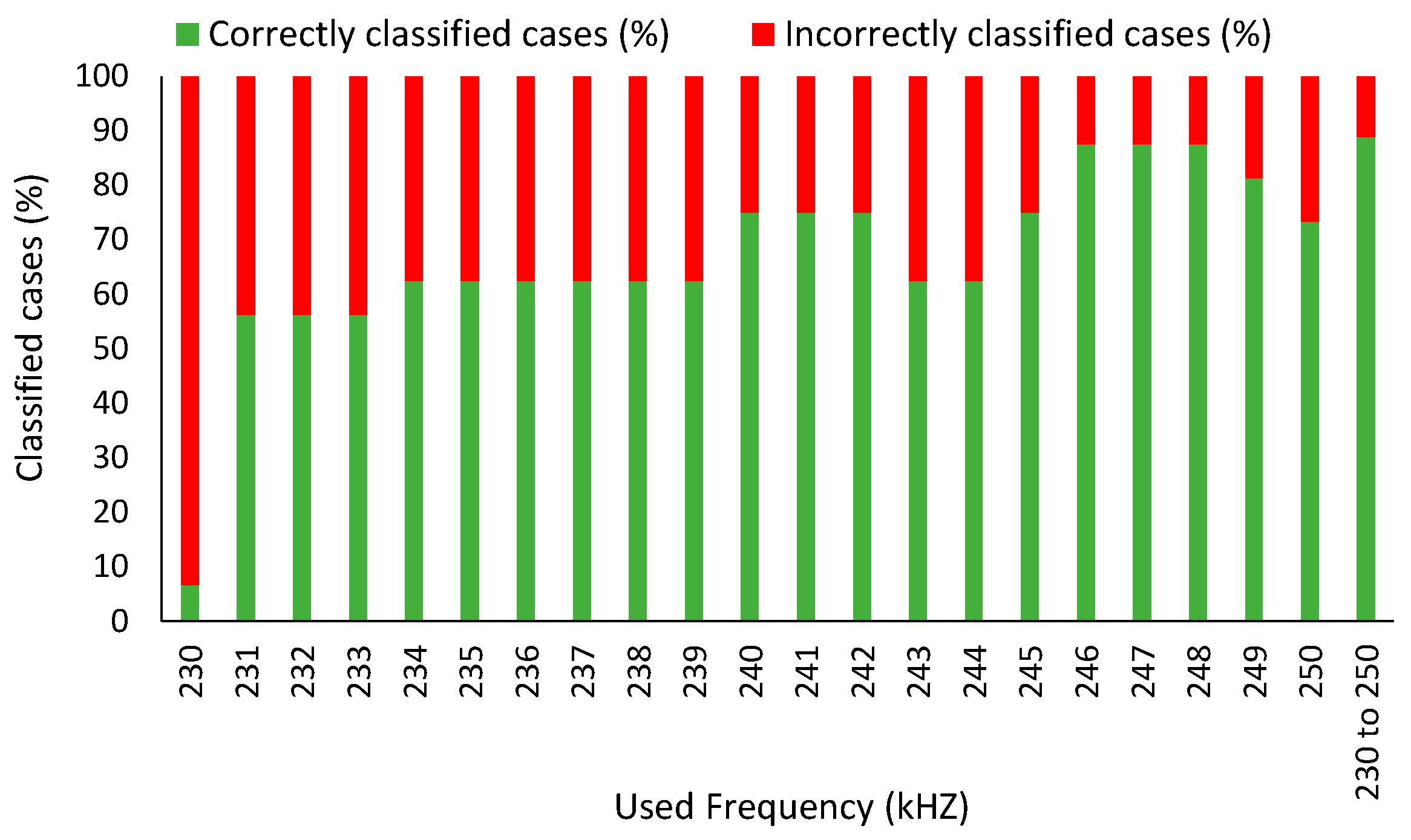
• Identify the most suitable frequency for the inductor operation.
• Assess any potential effect of temperature in the virtual sensor to determine whether temperature correction is necessary.

2. Materials and Methods

2.1. Laboratory Equipment

The laboratory equipment used to carry out the study is commercial laboratory equipment. In this case, a commercial pH meter (HI98129) has been used to check the pH of the samples. The accuracy of this is ±0.05 pH [46].

A magnetic stirrer (RSLab-11c) was used to homogenize the solutions. In addition, this device allows the maintenance of the temperature of the sample. Regarding the temperature variation of the samples, a laboratory water bath was used to heat and cool the samples. The samples’ temperature was measured using a digital thermometer (VENTIX ST-9263A). The accuracy is ±1 °C [47]. The samples were prepared in 1000 mL Erlenmeyer and decanted into 600 mL beakers. This has allowed the coil to be introduced into the sample.

A power supply has been used to feed the coil used, and an oscilloscope allows visualizing of the electrical signals and changes in the different media.

2.2. Reagents

The reagents used were 37% hydrochloric acid to establish the values of the acid pH scale. For the basic samples on the pH scale, 0.1 mol/L sodium hydroxide was used.

2.3. Coil Description

In order to develop the proposed device, it is used 2 coils of different sizes coiled over a PVC pipe and introduced into the water. The diameter of the PVC tube is 2.5 cm.

A coil, also known as an inductor, is an electronic device able to store energy in a magnetic field when an electrical current flows through it. The functioning of two coils can be understood by examining the concept of mutual inductance. As Parra et al. shown [38], the principle of operation of this sensor is based on the concept of mutual inductance between a powered coil ($L_{power}$) and an induced coil ($L_{induced}$). In this case, the sensor has two coils with lengths $H_{powered}$and $H_{induced}$and a number of spires of $N_{powered}$ and $N_{induced}$.with a given section (S). Additionally, the coils lack a ferromagnetic core. Instead of that, the internal part of the coils is occupied by water with concentrations of dissolved salts with a relative permeability ${\mu }_{r\_water}$. Equations (1) and (2) show the mathematical expression of the inductance of both coils.

$$L_{powered}\left(H\right)={\mu }_r\frac{N_{powered}{}^2·S}{H_{powered}}$$

(1)

$$L_{induced}\left(H\right)={\mu }_r\frac{N_{induced}{}^2·S}{H_{induced}}$$

(2)

On the other hand, the mutual inductance between two coils is determined by the number of turns in each coil, the size and shape of the coils, and the distance between the coils. When the current in the first coil changes, it creates an electromotive force and opposes the current change. The mutual inductance between two coils can be increased by increasing the number of turns in the coils, bringing the coils closer together, or making the coils larger. The mutual inductance $L_m$ between two coils can be calculated using the following expression:

$$L_m\left(H\right)=k\frac{N_{powered}·N_{induced}}{d},$$

(3)

where k is a constant depending on the type of core used, and d is the distance between the coils. Mutual inductance can also be positive or negative, depending on the orientation of the coils. If the coils are oriented in such a way that the magnetic flux generated by one coil passes through the other coil in the same direction, the mutual inductance is said to be positive. On the other hand, if the magnetic flux passes through the other coil in the opposite direction, the mutual inductance is said to be negative.

Table 1. Description of coils composing the sensor.

Coil	Section (mm)	Length (mm)	Wire Section (mm)	N°. Spires	Material
Powered	25	32	0.4	80	Enameled copper wire
Induced	25	16	0.4	40	Enameled copper wire

shows the measures of the coils, while Figure 1a shows a schematic of the disposition of both coils and their features. Finally, the distance between coils is 2 mm. The physical aspect of the coil during the measurements can be seen in Figure 1b. These coils have been based on previous studies. These studies show that the number of spires and the distance between the coils provide the most suitable values [38].

2.4. Samples Preparation

Different samples of different pH values (4, 5, 7, 8, 9, and 11) were prepared with distilled water. Buffer samples with pH values 4, 7, and 9 were used. A sachet of the buffer compound was added to 250 mL of distilled water to prepare these samples. After carrying out the dissolution, it was brought to a final volume of 500 mL. This volume allows the coil to be fully immersed. The rest of the pH values were adjusted using reagents such as hydrochloric acid and sodium hydroxide. To obtain the pH samples of 5, 8, and 11, the pH of the distilled water was adjusted using the acid and the base, respectively, until the desired pH was obtained.

Regarding the temperature, four different values were established (10, 20, 25, and 40 °C). The choice of these temperatures is due to the need to establish two extreme temperature values: a low temperature of 10 °C and a high temperature of 40 °C. The temperature of 20 °C is the ambient temperature in situ in the laboratory. Finally, the standard temperature, widely used in different fields for the development of tests, 25 °C, is tested too.

The beakers were sealed using Parafilm. This fact allows us to minimize the exchange of gases with the atmosphere. Regarding the control of temperature and pH, they were taken at the beginning, and the end of each sampling, and the average pH was calculated. Since measures were conducted over a short period of time, there were no big differences in temperature. These data-gathering times were below 5 min.

Table 2. pH measures according to temperature.

Integer Value of pH for the Analyses	pH of Samples for Each Temperature
	10	20	25	40
4	4.1	4.0	4.18	4.24
5	5.3	5.2	5.1	5.3
7	6.9	6.9	6.96	7.02
8	7.98	8.03	7.9	8.0
9	8.98	8.73	8.8	8.92
11	10.85	10.98	11.0	10.94

shows the exact pH values for each solution depending on temperature. However, the integer values have been set due to the sensitivity of the new sensor.

Three different water samples were used to verify the proposed sensor: distilled water, water and irrigation channel, and seawater. A pH ramp was conducted with all water samples, including pH values between 7 and 9. The pH of the water samples was modified by adding reagents in the natural water and by CO₂ exchange with the atmosphere for the distillate sample. The pH values were taken as integer values for verification.

2.5. Coil Powering

A function generator to create a sinus wave of 5 Vpp at different frequencies has been used to power the system and measure the results. This signal is in charge of inducing a current in the second coil. Using a digital oscilloscope, it is possible to measure the induced signal and the delay. Figure 2 shows the connection diagram of the coils, the function generator, and the oscilloscope.

2.6. Measuring Procedure

A set of frequencies to be tested for measuring the samples has been defined. First, the frequency at which the induced voltage is maximum has been identified; this is the Peak Frequency (PK). Based on previous studies [38], the response of the sensors is the maximum close to the PK. Thus, the tests started from 100 kHz to 500 kHz, measuring the induced voltage every 10 kHz. Nonetheless, these data were gathered every 1 kHz close to the peak frequency.

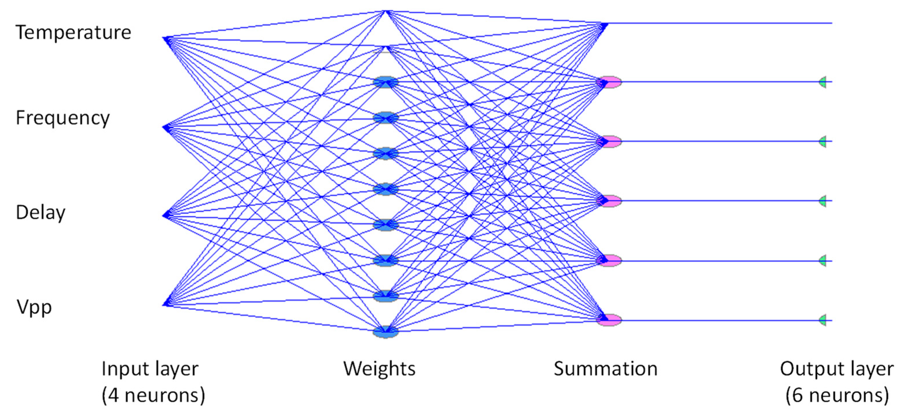
2.7. Data Processing and Analyses

The steps followed for data processing are defined in this subsection. First, X-YY plots were carried out to represent the Vpp and Frequency data of the tested coil for different pH and temperature values. The same graphs were created to identify the relationship between delay and frequency with pH and temperature. This is conducted to visualize these data and to check if this graphic suggests a possible correlation between Vpp or delay and pH value.

After visualizing these data from the X–Y plots, a two-way ANalysis Of VAriance (ANOVA) is selected to evaluate the influence of pH, frequency, and temperature on the obtained values of Vpp and the delay. Then, a multivariate analysis is performed to assess the correlation between the factors above (temperature, frequency, and pH) with delay and Vpp. The last step is to include the gathered data into a Probabilistic Neural Network (PNN) to classify these data according to the pH based on different input variables. In this step, the impact of temperature, delay, frequency, and Vpp on the accuracy of the PNN is considered. With these results, it will be possible to evaluate if the tested methodology can be used in the laboratory to classify the pH with all obtained data.

Nonetheless, to be used as a sensor, some adjustments are needed. First, it is necessary to filter these data according to the most common pH values in natural water bodies. In addition, the input information about the used frequencies will also be reduced, including only the frequencies for the best working range. In real applications, changing the frequency of the powering signal might be challenging. According to previous related work, the best working range is close to the PK. Thus, the input information in the system has been limited to frequencies close to the PK for evaluating the performance of the classification.

The last step will be identifying the sensor’s best Working Frequency (WF). This is necessary since the electronic configuration of the probe will allow its operation only at a certain frequency. To compare the performance of classification for the different frequencies, the percentage of correctly classified cases with a PNN is used to define the WK.

3. Results

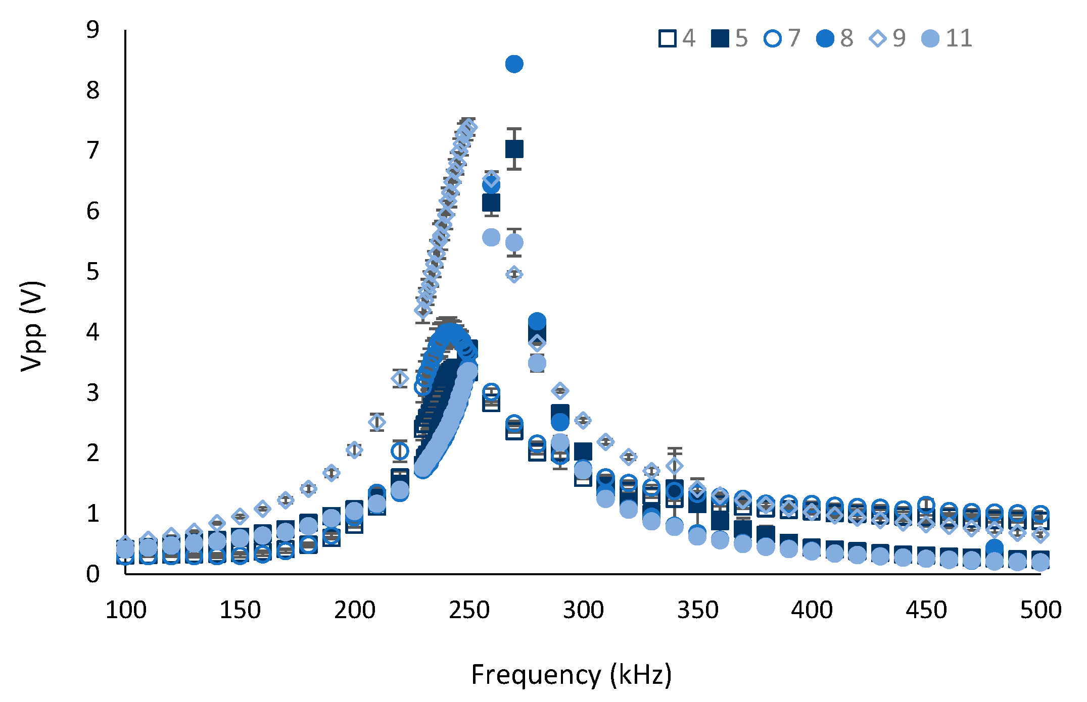
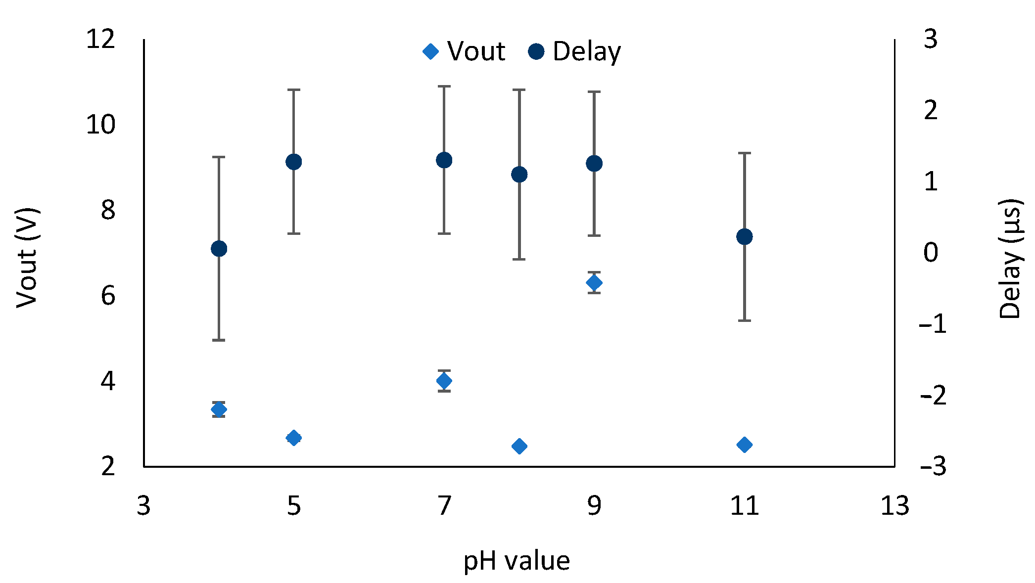
3.1. General Overview of Results

In the following graph (see Figure 3), the frequency in kilohertz (kHz) is plotted against the peak-peak voltage (Vpp) for different pH measurements. Note the maximum voltage is obtained when the frequency is around 220 kHz. Therefore, it is established that this is the working frequency for the coil used, also known as the working frequency zone. On the other hand, regarding the pH, it is observed that pH 9 and 11 present a higher peak than the rest of the values. The Vpp data indicated that at pH 8, the induced voltage is the lowest among tested solutions. According to the obtained data, it seems that there is a relationship between the pH value and Vpp since the values appear grouped. However, the obtained Vpp for the tested pH values is not listed in increasing or decreasing order.

In Figure 3, the effect of temperature is presented. As in Figure 4, the highest voltage peak that coincides with the working frequency is observed. It is observed that there is no relationship between temperature and voltage since the temperatures are not grouped. It is observed that higher voltage occurs for the temperature of 40 °C.

The following graph (see Figure 5) shows the frequency versus the delay in milliseconds and the different pH values. No apparent differences are observed between the values obtained. However, it is observed that the retardation for pH values 5 and 9 is farther away. In Figure 6, the effect of temperature is seen. The effect of temperature on the retardation for the different pH values cannot be observed in this graph.

3.2. ANOVAs and PNN with All the Data

In this subsection, the results of the two-way ANOVA for Vpp and delay are analyzed. Then, the PNN output is presented and analyzed.

First, the results of the two two-way ANOVA for Vpp and Duncan’s Multiple Range Test for Temperature and pH are presented in

Table 3. Two-Way ANOVA results for Vpp with all gathered data.

Source of Variation	SS (/107)	Df	MS(/105)	F	p-Value 1
Temperature	1.31835	3	43.945	8.38	<0.0000
pH	40.3099	5	806.197	153.71	<0.0000
Frequency	259.894	58	448.093	85.43	<0.0000
Error	64.5657	1231	5.24498
Total	368.557	1297

¹ Results for 95% of confidence.

,

Table 4. Duncan’s Multiple Range Test for Temperature of Two-Way ANOVA results for Vpp with all gathered data.

Temperature (°C)	Cases	Mean Vpp Value
10	354	1837.21 a
20	354	1956.36 b
25	354	1965.19 b
40	236	2152.07 c

^a Different letters indicate different groups.

and

Table 5. Duncan’s Multiple Range Test for pH of Two-Way ANOVA results for Vpp with all gathered data.

pH	Cases	Mean Vpp Value
11	177	1563.97 a
8	177	1636.48 ab
5	236	1676.77 ab
4	236	1771.17 b
7	236	2062.17 c
9	236	3155.67 d

^a Different letters indicate different groups.

. Table 3 includes the Summation of Squares (SS), the Degrees of freedom (Df), the Mean Square (MS), the F-value (F), and the p-value. The results summarized in Table 3 indicate that all factors significantly affect the variability of the Vpp according to the p-values, which are lower than 0.005. Table 4 and Table 5 include the number of cases and the mean Vpp value. In addition, the groups generated according to the mean values are indicated by superscript letters. The groups were defined according to the value for Duncan’s Multiple Range Test. The tests were repeated twice, one for each factor, the pH or the temperature. The results in Table 4 pointed out that there are three groups for the temperatures, temperature 25 °C and temperature 20 °C in the same group. Meanwhile, Table 5 shows the results of grouping Vpp data according to the pH values. In this case, four groups are found, and pH values of 8 and four are included in the same group.

The results of the two two-way ANOVA for the delay and Duncan’s Multiple Range Test for Temperature and pH are presented in

Table 6. Two-Way ANOVA results for the delay with all gathered data.

Source of Variation	SS SS (/107)	Df	MS SS (/106)	F	p-Value 1
Temperature	2.2366	3	7.45532	6.02	0.0005
pH	14.2699	5	28.5398	23.06	<0.0000
Frequency	104.076	58	17.9442	14.50	<0.0000
Error	152.37	1231	1.23778
Total	274.215	1297

¹ Results for 95% of confidence.

,

Table 7. Duncan’s Multiple Range Test for Temperature of Two-Way ANOVA results for the delay with all gathered data.

Temperature (°C)	Cases	Mean Vpp Value
10	354	140.984 a
25	354	269.954 ab
40	236	411.832 bc
20	354	473.888 c

^a Different letters indicate different groups.

and

Table 8. Duncan’s Multiple Range Test for pH of Two-Way ANOVA results for the delay with all gathered data.

pH	Cases	Mean Vpp Value
11	177	−0.560028 a
8	177	0.161441 a
5	236	82.464 a
9	236	304.29 b
7	236	778.511 c
4	236	780.122 c

^a Different letters indicate different groups.

. According to the p-values of Table 6, all factors significantly affect the delay’s variability. The results in Table 7 indicate that there are three groups for the temperatures. Nonetheless, all temperatures are classified differently. Regarding Table 8, the second Duncan’s Multiple Range Test results pointed out that there are only three groups for the pH. The pH data equal to 5, 8, and 11 are classified in the same group.

These initial results suggest that even though the two studied factors, temperature, and pH, significantly affect both Vpp and delay, it might not be possible to classify the samples using a single parameter (Vpp or delay). Thus, for the combination of both parameters and the factors which can be easily measured with existing physical sensors, the temperature is used as the input neurons in a PNN. The frequency is also added as an input neuron since it affects the delay and Vpp. The first scheme for the first PNN tested can be seen in Figure 7. In this case, all data are used for the classification; the PNN is trained with jackknifing, which is 0.01797 and assumes an equal previous probability and equal cost of error for all groups. The confusion matrix, which summarises the results when all data are used, can be seen in

Table 9. Classification results of PNN using all cases and temperature, frequency, Vpp, and delay as input neurons.

Current pH	Cases	Classified as pH
		4	5	7	8	9	11
4	236	45.76% (108)	0%	46.19% (109)	0.85% (2)	6.36% (15)	0.85% (2)
5	236	1.27% (3)	43.22% (102)	0.85% (2)	27.54% (65)	6.36% (15)	20.76% (49)
7	236	49.15% (116)	0.42% (1)	44.07% (104)	0.42% (1)	5.93% (14)	0%
8	177	0.56% (1)	23.16% (41)	0%	6.21% (11)	2.82% (5)	67.23% (119)
9	236	8.47% (20)	10.17% (24)	9.75% (23)	2.54% (6)	68.64% (162)	0.42% (1)
11	177	0.56% (1)	22.03% (39)	0%	66.10% (117)	0%	11.30% (20)
Total correctly classified 39.06%

.

Considering the experience in the past with similar PNN and data [48], the reduction in input neurons is evaluated. Thus, the temperature and the frequency are deleted individually and jointly in three new PNNs. The results of the PNN when temperature, output voltage, and delay are used are shown in

Table 10. Classification results of PNN using all cases and temperature, Vpp, and delay as input neurons.

Current pH	Cases	Classified as pH
		4	5	7	8	9	11
4	236	62.29% (147)	2.97% (7)	30.93% (73)	1.27% (3)	1.69% (4)	0.85% (2)
5	236	2.54% (6)	52.97% (125)	2.97% (7)	14.83% (35)	6.78% (16)	19.92% (47)
7	236	27.12% (64)	2.97% (7)	66.10% (156)	1.27% (3)	2.12% (5)	0.42% (1)
8	177	2.26% (4)	23.16% (15)	0%	44.07% (78)	2.26% (4)	42.94% (76)
9	236	2.97% (7)	8.05% (19)	12.71% (30)	6.78% (16)	65.68% (155)	3.81% (9)
11	177	1.69% (3)	12.99% (23)	0.56% (1)	66.10% (77)	2.26% (4)	38.98% (69)
Total correctly classified 56.24%

. It is possible to see that the percentage of correctly classified data increases to 56.24%. In this case, the jackknifing value is 0.0148. When the frequency, delay, and output voltage are the input neurons, the percentage of correctly classified data reaches 73.57%. These data can be seen in

Table 11. Classification results of PNN using all cases and frequency, Vpp, and delay as input neurons.

Current pH	Cases	Classified as pH
		4	5	7	8	9	11
4	236	82.63% (195)	0.42% (1)	16.10% (38)	0%	0.42% (1)	0.42% (1)
5	236	0%	63.14% (149)	0.42% (1)	13.56% (32)	6.78% (16)	16.10% (38)
7	236	36.44% (86)	0%	61.02% (144)	0%	2.12% (5)	0.42% (1)
8	177	0.56% (1)	2.26% (4)	0%	75.14% (133)	0.56% (1)	21.47% (38)
9	236	3.81% (9)	2.12% (5)	2.54% (6)	0%	91.53% (216)	0%
11	177	0.56% (1)	5.65% (10)	0.56% (1)	26.55% (47)	0%	66.67% (118)
Total correctly classified 73.57%

, and the jackknifing value is 0.133.

Finally, if only delay and the output voltage are used, the percentage of correctly classified data drops to 68.49%, see

Table 12. Classification results of PNN using all cases and Vpp and delay as input neurons.

Current pH	Cases	Classified as pH
		4	5	7	8	9	11
4	236	73.73% (174)	3.81% (9)	19.49% (46)	0.42% (1)	1.27% (3)	1.27% (3)
5	236	1.27% (12)	55.93% (132)	3.39% (8)	10.17% (24)	8.90% (21)	16.53% (39)
7	236	24.15% (57)	4.24% (10)	67.37% (159)	0.42% (1)	2.12% (5)	1.69% (4)
8	177	1.13% (2)	3.95% (7)	0.56% (1)	71.75% (127)	1.69% (3)	20.90% (37)
9	236	1.69% (4)	8.05% (19)	5.51% (13)	3.81% (9)	78.81% (186)	2.12% (5)
11	177	1.13% (2)	12.43% (22)	0.56% (1)	22.03% (39)	1.13% (2)	62.71% (111)
Total correctly classified 68.49%

. The jackknifing value for that last case is 0.006. It is important to remark that in all cases, the samples with pH 11 and pH 8 are the ones with the higher percentage of incorrectly classified data. The differences in correctly classified cases among the different evaluated input neurons indicate that including delay, output voltage, and frequency is the one that offered the most accurate results. It can be caused by the experimented difficulties in maintaining the temperature stable along the measures. Thus, the temperature data case supposes a noise in the PNN.

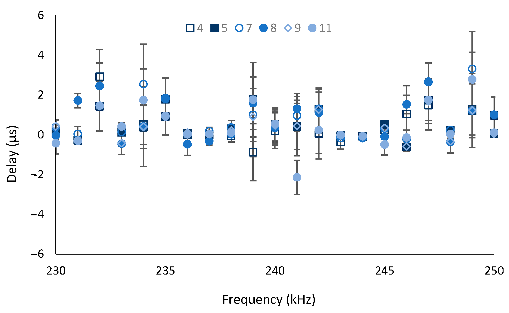
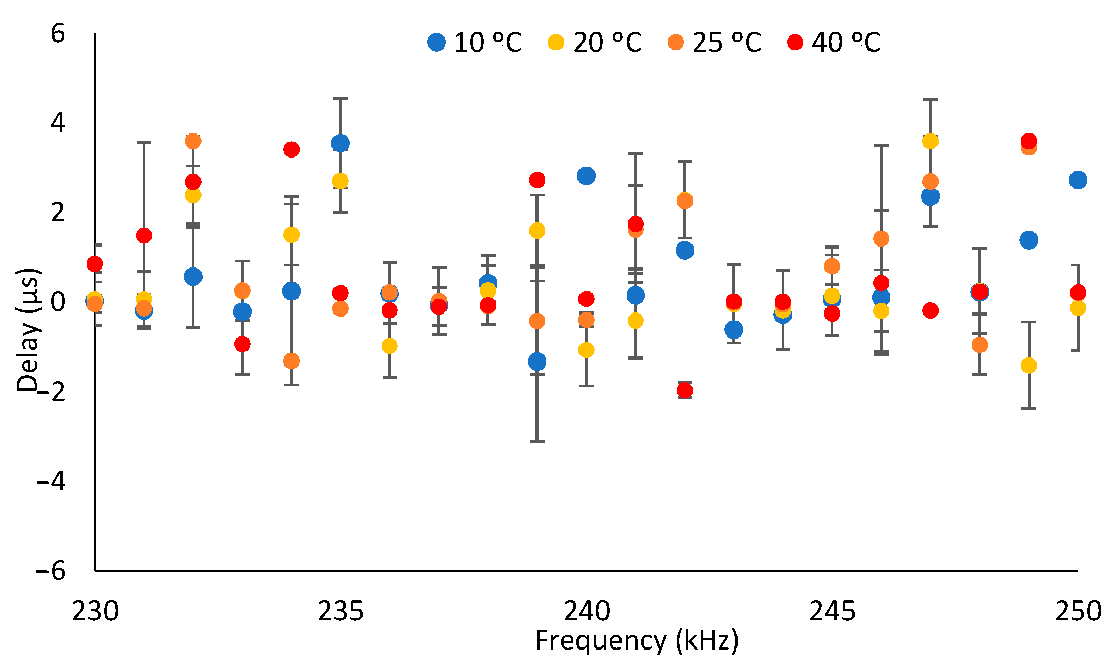
3.3. General Overview of Results of the Selected Range

Figure 8 shows these obtained data for the selected range. In the selected range, these obtained data are only those obtained in the area of the working frequency. In this case, the Vpp values for each pH value in the frequency range are represented. It is observed that the pH values appear grouped and that pH 9 is the one with the highest Vpp value. On the other hand, pH 8 is the one that shows the lowest Vpp values.

In Figure 9, the effect of temperature is shown. It is observed that the temperature values are grouped and that the temperatures 20 °C and 25 °C present a higher voltage for a particular pH value.

Figure 10 represents the selected frequency range against the delay for the different pH values. It is observed that when the frequency values are higher and close to the working frequency, the delay values go from positive to negative values. As in Figure 11, the frequency is a function of the delay considering the temperature. No relationship with temperature is observed in this graph.

The Vpp data and delay obtained at the PF for the different pH values can be seen in Figure 12. The PF has been selected according to the Vpp at a pH of 7; the PF is 242 kHz. The PF varies along the tested pH values. This confirms the above information that there is no apparent linear regression between pH and obtained data. Thus, other types of approaches are used for further analyses.

3.4. ANOVAs and ANN with Selected Data

This subsection analyses the results of the two-way ANOVA for Vpp and delays for these selected data. Then, the PNN output is presented and analyzed for all selected data. Finally, the evaluation of the possibility of a single-frequency use for the classification of pH is detailed.

Initially, the two two-way ANOVA results for Vpp and Duncan’s Multiple Range Test for temperature and pH are presented. These results can be seen in

Table 13. Two-Way ANOVA results for Vpp with selected data.

Source of Variation	SS (/107)	Df	MS (/106)	F	p-Value
Temperature	6.06042	3	20.2014	24.40	<0.0000
pH	22.9289	4	57.3222	69.23	<0.0000
Frequency	41.9108	20	20.9554	25.31	<0.0000
Error	25.3368	306	0.827999
Total	102.38	333

¹ Results for 95% of confidence.

,

Table 14. Duncan’s Multiple Range Test for Temperature of Two-Way ANOVA results for Vpp with selected data.

Temperature (°C)	Cases	Mean Vpp Value
10	83	326.848 a
25	105	847.02 b
40	41	1287.07 c
20	105	1439.08 c

^a Different letters indicate different groups.

and

Table 15. Duncan’s Multiple Range Test for pH of Two-Way ANOVA results for Vpp with selected data.

pH	Cases	Mean Vpp Value
8	63	9.33551 a
5	63	266.996 ab
9	42	585.956 b
4	83	1968.77 c
7	83	2043.96 c

^a Different letters indicate different groups.

. Regarding data from Table 13 pointed out that the three factors have a significant effect on the variability of the Vpp; all p-values are lower than 0.005. On the one hand, in Table 14, three groups are found, and data from 20 and 40 °C are classified into the same group. On the other hand, data from Table 15 indicate three groups, some merging data from different pH levels.

To conclude the ANOVAs, the results of the two two-way ANOVA for the delay and Duncan’s Multiple Range Test for Temperature and pH when selected data are used are presented in

Table 16. Two-Way ANOVA results for the delay with selected data.

Source of Variation	SS (/107)	Df	MS (/105)	F	p-Value
Temperature	1.35745	3	45.2485	42.47	<0.0000
pH	33.4439	4	836.098	784.68	<0.0000
Frequency	6.34787	20	31.7393	29.79	<0.0000
Error	3.26051	306	1.06552
Total	48.6782	333

¹ Results for 95% of confidence.

,

Table 17. Duncan’s Multiple Range Test for Temperature of Two-Way ANOVA results for the delay with selected data.

Temperature (°C)	Cases	Mean Vpp Value
10	83	3224.96 a
20	105	3576.92 b
25	105	3587.66 b
40	41	3923.76 c

^a–c Different letters indicate different groups.

and

Table 18. Duncan’s Multiple Range Test for pH of Two-Way ANOVA results for the delay with selected data.

pH	Cases	Mean Vpp Value
8	63	2514.51 a
5	63	2674.03 b
4	83	3095.34 c
7	83	3751.87 d
9	42	5855.87 e

^a–e Different letters indicate different groups.

. According to Table 16, again, all factors significantly affect the delay’s variability. Table 17 indicates that there are three groups for the temperatures. The temperatures of 20 and 25 °C are classified in the same group. Finally, the results of Table 1 pointed out that there are five groups for the pH, one for each pH value.

The results from these statistical analyses indicate that the classification of data according to the two-way ANOVAs when data are filtered improved. A reduction in data variability due to deleting one of the pH samples and focusing on the frequencies close to the PF improved the results. The simplified data are now used as input for the PNN. According to the results of the previous subsection, the comparison of correctly classified cases for the different input information is presented in

Table 19. Correctly classified cases with PNN using different input information for the selected data.

pH	Cases	Correctly Classified
		All	Vpp, Delay, and Temperature	Vpp, Delay, and Frequency	Vpp and Delay
4	83	98.7952	96.3855	96.3855	95.1807
5	63	66.6667	69.8413	58.7302	66.6667
7	83	98.7952	95.1807	89.1566	87.9518
8	63	60.3175	65.0794	93.6508	96.8254
9	42	100.0	100.0	100.0	100.0
Total	334	85.63	85.63	87.42	88.92

. Comparing the results of Table 19 with the results of initial PNNs, Table 8, Table 9, Table 10 and Table 11, it is possible to affirm that the percentage of correctly classified cases has improved considerably. As in the other case, the accuracy improves when the temperature is excluded from input data (87.42% of correctly classified cases compared with 85.63%). In this case, the maximum percentage of correctly classified cases, 88.92%, is attained when only delay and output voltage are used.

Finally, to select the best WF, PNNs are calculated for each of the frequencies in the PNN of Table 18. The results can be seen in Figure 13, which represents the correctly classified cases for these data corresponding to each frequency in the x-axis. When all data are used, 88.92% of cases are correctly classified. The best WF are 246, 247, and 248 kHz. For those frequencies, the correctly classified cases are 87.5%. There is a reduction in less than 1.5% of cases. Any of these frequencies is recommended for the pH monitoring sensor.

3.5. Verification with New Water Samples

The results for the new water samples are presented in terms of correctly classified cases with the ANN model obtained at 274 kHz. When the obtained Vpp and delays for water samples with diverse pH values of all water sources are included in the verification, the percentage of correctly classified cases decrease to 33%. When only data about distilled water, which pH varies due to the CO₂ exchange with the atmosphere and which has a similar composition to calibration samples, the percentage reaches 83%. In this case, the errors were linked to the values which were a bit below 7. It might be caused because this stage is when the pH varies faster due to the exchange of CO₂ with the atmosphere, which might impact the measurements. In natural and water samples, it might not be a problem since natural water use is equilibrated with the atmosphere. This suggests that more experiments are needed to ensure an acceptable percentage of classified cases with different water sources.

4. Discussion

4.1. General Findings

The utmost relevant results are the following:

• The use of Vpp and delay of the generated magnetic field of a water core coil used as input data for the PNN can serve as a virtual pH sensor, attaining 88.9% of correctly classified cases and 83% in the verification tests with new samples.
• The best WF for the inductor is 246, 247, and 248 kHz; any of these frequencies offer the same percentage of correctly classified cases in the PNN.
• The differences between using a single frequency, see frequencies above, and using a range of frequencies represent a decrease lower than 1.5% of the correctly classified cases with the PNN.
• Even though, according to two-way ANOVA results, the temperature significantly affects the variation of delay and Vpp, once data of both Vpp and delay are introduced in the PNN, the results improve when the temperature is excluded from the input neurons. The improvement of correctly classified cases when the temperature is excluded represents 43% when all data are used and 2% when selected data are used.

This paper’s main novelty is identifying a copper coils-based virtual sensor for pH monitoring, being the first pH virtual sensor for water samples. This covers an important gap in the current literature since virtual sensors were applied for multiple chemical parameters but not for pH so far. The impact of this virtual sensor for coastal water monitoring in locations in which probes are cleaned, calibration, and membrane replacement will suppose better sensor networks for water quality. The low cost of these sensors and their low maintenance needs will increase the available information about water quality, helping the water managers to; (i) manage their valuable resources properly, (ii) classify the environmental impacts suffered along the coastal line, and (iii) identify abnormal situations in marine reserves using early warning systems.

As mentioned before, existing pH sensors are based on the use of chemical reactions of the use of electrodes and membranes, such as the glass membrane. Several proposals have appeared in recent years due to the requirements of pH monitoring in different areas and the high maintenance requirements of the glass membrane pH sensors. Those proposals are based on different chemical and photochemical reactions of H+ with the sensor. For that purpose, a wide variety of chemical compounds are used; in

Table 20. Summary of recent pH sensors.

Operation Principle	Possibility to WSN	pH Range (N° of Tested pHs)	Temperature Range (N° of Temperatures)	Classification	Accuracy	Year	Ref.
Polymer + Flourescense	No	2–11 (17)	-	Two regression models	R2 = 0.99	2018	[49]
Polymer + Flourescense	No	3.8–8.7 (5)	9.85–69.85	Regression model	R2 = 0.99	2019	[50]
Polymer + Flourescense	No	4–12 (9)	-	Regression model	R2 = 0.99	2022	[51]
Polymer + Flourescense	No	9–13 (5)	-	Regression model	R = 0.98	2019	[52]
Polymer + Flourescense	No	0.04–8.69 (16)	-	Regression model	R2 = 0.99	2020	[53]
Polymer + Refractive index	Apparently yes	1–12 (5)	20–40 (5)	Linear regression	-	2018	[54]
Electrode + Potentiometric	Yes	6–9 (4)	-	Regression model	R2 = 0.98	2019	[55]
Polymer + Potentiometric	Yes	6.09–8.92 (4)	-	-	-	2022	[56]
Electrode + Potentiometric	Yes	4.3–9 (5)	25–45 (3)	Regression model	R2 = 0.99	2019	[57]
Electrode + Potentiometric	Yes	2–12 (6)	-	Regression model	-	2020	[58]
ISFET	Yes	2–10 (9)	23–53 (4)	Regresion model	R2 = 0.99	2021	[59]
Electromagnetic field	Yes	4–9 (5)	10–40 (4)	PNN	R2 = 0.69	2023	This work

, a summary of some of those sensors is outlined. The aim of adding Table 20 is to compare the accuracy of existing pH sensors, their calibration range, and the inclusion of temperatures in the calibrations, among others, with the proposed sensor and calibration conducted in this paper. All the included sensors are developed for liquid monitoring. Although all the sensors are developed for liquid monitoring, some cannot be adapted or included in WSN since they are for a single-use or the preparation conditions prevent their use for water quality monitoring. These proposals for pH monitoring are based on the use of polymers introduced in the samples and the posterior use of fluorescence measuring. Thus, these proposals cannot be used in WSN since the continuous need for reagents (polymer and others) is not compatible with the WSN [49,50,51]. Moreover, these reagents might be toxic or harmful to aquatic life and the environment. Other examples are based on sol-gel polymers, and their maintenance needs are incompatible with the water quality monitoring in WSN [52,53].

There are other types of polymers that are not similar to the aforementioned ones. The solutions presented in [54] are based on hydrogel-coated optical fiber surface plasmon resonance. In this case, the polymer is immobilized with a thin silver film. Thus, according to the structure of the sensor, it might be implemented in a WSN. Nonetheless, it will be necessary to evaluate the performance of the sensor along with the time and the requirements in the light transmission measurement in the framework of a WSN for water quality monitoring. Other pH-measuring solution sources are based on electrodes, such as [55,56,57,58]. Different types of elements are used for the creation of electrodes, such as graphite [55,56], palladium [57], and even a combination of different elements [58]. These cases are easier to adapt to its use in a WSN. These sensors can be used for a long time, and since their response is a change in the potentiometric variable of the electrode, they can be easily integrated into a sensor node. Finally, the most typical solutions for pH monitoring in WSN are the Ion Sensitive Field-Effect Transistors (ISFET) [59]. The ISFET sensors have been used in WSN in recent years as the best solution for pH measurement. Nonetheless, the use of metallic elements, the miniaturized size of the sensing element, its dependence on the temperature, and other aspects of this type of sensor make the ISFETs an incomplete solution for some environments. The water turbidity and the presence of phytoplankton and epiphytes make its operation difficult in natural aquatic environments.

Among the presented solutions in Table 20, very few have considered the effect of temperature. The authors of [50,54,57,59] studied the effect of variations in temperature on the pH measurement. Only in [49,59] the temperature compensation is necessary. The obtained results suggest that the temperature explains part of the variability of delay and Vpp, the parameters measured. Nevertheless, when both parameters are combined in the PNN, the temperature is not necessary for the correct data classification.

Considering the pH range used for the calibration of the proposed sensor, 4 to 9, is aligned with some of the used ranges in other publications, such as [50,55,56,57]. In addition, these values cover the expected pH values in seawater samples, between 7 and 8, according to [60]. In this work, lower pH values are included in order to cover the expected punctual pH values due to acidification processes linked to pollution events from industries, which might drop even to 3.6 [61] and the acidification of the oceans due to CO₂ [62].

The presented solutions for pH monitoring represent the existing efforts in the existing literature. Even though many papers can be found in which a pH sensor is used for water quality monitoring, very few show the design and calibration of the sensing element. Several examples of pH monitoring solutions can be found in the following review [1,35,63,64,65]. Other examples of pH monitoring based on imaging can be found in [66,67,68]. Nevertheless, these methods are based on the specific characteristics of the studied area and the colored organic matter, which is the main source of pH. However, these methods become useless for general water monitoring.

Finally, regarding the classification approach and attained accuracy, the differences in the classification of chemical sensors and the fact that the proposed sensor is a virtual sensor prevent a fair comparison. Thus, no comparison is made with the sensors in Table 20. The comparison of accuracy is conducted with other virtual sensors for other parameters and alternative methods for pH monitoring. The R2 of these methods is much lower than the ones reported in Table 20. Some examples of R2 values of regression models of alternative ways of pH monitoring are 0.89 [67] and 0.69 [68]; in both cases, pH was estimated according to the hyperspectral images of the water body. However, as mentioned before, this method cannot be used for general water quality monitoring. Focusing on the virtual sensors, the following R2 can be found for calcium from 0.94 [42], NO3 0.89 [69], total reactive phosphorus 0.32 [69], total phosphorus 0.74 [69] and 0.71 [45], chemical oxygen demand 0.70 [45]. The proposed virtual pH sensors have an R2 of 0.69. This value is similar to other virtual sensors.

4.2. Limitations of Presented Results and Possible Future Solutions

The most relevant limitation of the proposed work is the relatively lower accuracy compared with existing methods. The proposed sensor correctly classifies 88.9% of cases. Testing coils will improve this relatively low accuracy with other configurations in future work. In conductivity meters based on inductors, the coil configuration changes improve accuracy. In addition, more calibration samples will be used to add more data for the PNN and improve its accuracy.

Among other samples with different pH and different temperature levels, the effect of additional parameters, such as salinity, turbidity, organic matter, and dissolved oxygen, will be considered. Thus, the proposed sensor system will be able to evaluate the effect of other parameters and the need for compensations. All data will be included in the PNN in order to increase the dataset.

The other limitation is the use of artificial samples and buffers. Nonetheless, most of the papers surveyed in Table 18 used buffers. In order to improve the accuracy of the pH sensor in natural seawater, in future work, samples of seawater, freshwater, and brackish water will be collected and used for the evaluation of sensor performance. The first step will consist of creating several pH ramps in water samples with different ionic strengths and generating different ANN models for each type of water. Thus, we will combine the pH sensors with other sensors to characterize the type of water in order to apply the corresponding ANN. A second step can consist of creating a general ANN with all pH ramps being the type of water one of the inputs for the ANN.

Regarding durability, the sensors based on copper coils have been tested many times. Even though data about their durability in underwater environments, existing data about their durability in other environments demonstrated that sensors could be used after many years. In underwater environments, factors such as biofouling, sediments or organic matter deposition, or the accumulation of air bubbles in the core might be a challenge. The biofouling will alter the behavior of the sensor; it is expected that the effect of biofouling in the sensor will drift in the measurements. It can be possible to model this drift and correct it. Anyway, the most efficient solution is to evaluate methods to reduce biofouling as performed in other sensors, such as using UV light [70] or magnetic mechanisms [71]. Considering that the sensors are based on electromagnetic fields, it must be evaluated if generated magnetic field can limit the biofouling growth.

Finally, the last limitation which will be overcome in the subsequent studies is the measurement of additional physical parameters. Regarding the inductor, the delay and the Vpp are already measured. In previous studies, the Vpp was related to the conductivity [38], but the delay has no relation with conductivity according to the existing literature and other conducted experiments. Additional parameters, such as frequency, can be measured in the future. Nonetheless, in this experiment and previous ones, no differences in frequencies are detected. No other physical parameters can be measured in the double inductor system. Thus, the other physical parameters might include optical effects such as light abortion at different wavelengths.

5. Conclusions

One of the main parameters measured in water quality monitoring is pH. Considering the wide variety of scenarios in which pH is measured, the requirements for pH sensors are variable. Most pH sensors and probes are based on a glass membrane, which must be cleaned after data collection. Moreover, these types of sensors need calibration from time to time. Therefore, using virtual sensors is a good option for this environment. In addition to their low cost, these virtual sensors are low maintenance and might not need to be calibrated.

This paper describes developing and calibrating a virtual pH sensor to detect abnormal situations in coastal areas. For this, an inductor has been tested as a virtual pH sensor. Therefore, samples with different pH values (4, 5, 7, 8, 9, and 11) and at different temperatures (10, 20, 25, and 40 °C). Finally, a pH range has been selected, and the value of pH 11 has been eliminated. When data from a selected dataset, without a pH value of 11 and focusing on the range of frequencies with better accuracy, is used as the input layer, the percentage of correctly classified cases reaches 85.63%. When the temperature is excluded from the analyses, the percentage of correctly classified cases improves to 87.42%. When only the delay and output voltage data are used, the percentage of correctly classified is 88.92%. It has been obtained that the best WF for the selected coil is 246, 247, and 248 kHz. For those frequencies, the percentage of correctly classified is 87.50%.

In future work, the sensor will be tested with different pH and temperature values to generate a larger dataset for the PNN in order to achieve higher precision and accuracy, including intermediate values of already tested solutions and new solutions with pH values of 6 and 10. Other types of sensors, such as oxidation-reduction and conductivity sensors, will be jointly deployed to detect possible interferences between the sensors. Measures will be established in different study areas. In the subsequent experiments, the deployment of the used probe to detect the pH will be conducted in different underwater environments to evaluate the durability and stability of the probe. Finally, the design of an electronic circuit that allows the implementation of the virtual sensor in natural environments and its subsequent adaptation into a sensor node of a WSN will be assessed.

References

1. Steinegger, A.; Wolfbeis, O.S.; Borisov, S.M. Optical Sensing and Imaging of pH Values: Spectroscopies, Materials, and Applications. Chem. Rev. 2020, 120, 12357–12489. [Google Scholar] [PubMed]
2. Majhi, P.K.; Kothari, R.; Arora, N.K.; Pandey, V.C.; Tyagi, V.V. Impact of pH on Pollutional Parameters of Textile Industry Wastewater with Use of Chlorella pyrenoidosa at Lab-Scale: A Green Approach. Bull. Environ. Contam. Toxicol. 2021, 108, 485–490. [Google Scholar] [PubMed]
3. Ziara, R.M.; Miller, D.N.; Subbiah, J.; Dvorak, B.I. Lactate wastewater dark fermentation: The effect of temperature and initial pH on biohydrogen production and microbial community. Int. J. Hydrogen Energy 2018, 44, 661–673. [Google Scholar]
4. Galan, I.; Müller, B.; Briendl, L.G.; Mittermayr, F.; Mayr, T.; Dietzel, M.; Grengg, C. Continuous optical in-situ pH monitoring during early hydration of cementitious materials. Cem. Concr. Res. 2021, 150, 106584. [Google Scholar]
5. Briendl, L.G.; Grengg, C.; Müller, B.; Koraimann, G.; Mittermayr, F.; Steiner, P.; Galan, I. In situ pH monitoring in accelerated cement pastes. Cem. Concr. Res. 2022, 157, 106808. [Google Scholar]
6. Boczkaj, G.; Fernandes, A. Wastewater treatment by means of advanced oxidation processes at basic pH conditions: A review. Chem. Eng. J. 2017, 320, 608–633. [Google Scholar]
7. Goulart, D.A.; Pereira, R.D. Autonomous pH control by reinforcement learning for electroplating industry wastewater. Comput. Chem. Eng. 2020, 140, 106909. [Google Scholar] [CrossRef]
8. Sabzi, S.; Arribas, J.I. A visible-range computer-vision system for automated, non-intrusive assessment of the pH value in Thomson oranges. Comput. Ind. 2018, 99, 69–82. [Google Scholar]
9. Pourdarbani, R.; Sabzi, S.; Kalantari, D.; Arribas, J.I. Non-destructive visible and short-wave near-infrared spectroscopic data estimation of various physicochemical properties of Fuji apple (Malus pumila) fruits at different maturation stages. Chemom. Intell. Lab. Syst. 2020, 206, 104147. [Google Scholar]
10. Alizadeh-Sani, M.; Mohammadian, E.; Rhim, J.W.; Jafari, S.M. pH-sensitive (halochromic) smart packaging films based on natural food colorants for the monitoring of food quality and safety. Trends Food Sci. Technol. 2020, 105, 93–144. [Google Scholar]
11. Tirtashi, F.E.; Moradi, M.; Tajik, H.; Forough, M.; Ezati, P.; Kuswandi, B. Cellulose/chitosan pH-responsive indicator incorporated with carrot anthocyanins for intelligent food packaging. Int. J. Biol. Macromol. 2019, 136, 920–926. [Google Scholar]
12. Jiao, S.; Lu, Y. Soil pH and temperature regulate assembly processes of abundant and rare bacterial communities in agricultural ecosystems. Environ. Microbiol. 2019, 22, 1052–1065. [Google Scholar] [PubMed]
13. Zhou, W.; Han, G.; Liu, M.; Li, X. Effects of soil pH and texture on soil carbon and nitrogen in soil profiles under different land uses in Mun River Basin, Northeast Thailand. PeerJ 2019, 7, e7880. [Google Scholar] [PubMed] [Green Version]
14. Bouaroudj, S.; Menad, A.; Bounamous, A.; Ali-Khodja, H.; Gherib, A.; Weigel, D.E.; Chenchouni, H. Assessment of water quality at the largest dam in Algeria (Beni Haroun Dam) and effects of irrigation on soil characteristics of agricultural lands. Chemosphere 2018, 219, 76–88. [Google Scholar]
15. van Rooyen, I.L.; Nicol, W. Optimal hydroponic growth of Brassica oleracea at low nitrogen concentrations using a novel pH-based control strategy. Sci. Total Environ. 2021, 775, 145875. [Google Scholar]
16. Huan, J.; Li, H.; Wu, F.; Cao, W. Design of water quality monitoring system for aquaculture ponds based on NB-IoT. Aquac. Eng. 2020, 90, 102088. [Google Scholar]
17. Gao, G.; Xiao, K.; Chen, M. An intelligent IoT-based control and traceability system to forecast and maintain water quality in freshwater fish farms. Comput. Electron. Agric. 2019, 166, 105013. [Google Scholar]
18. Staudinger, C.; Strobl, M.; Breininger, J.; Klimant, I.; Borisov, S.M. Fast and stable optical pH sensor materials for oceanographic applications. Sensors Actuators B Chem. 2019, 282, 204–217. [Google Scholar]
19. Jiang, L.-Q.; Carter, B.R.; Feely, R.A.; Lauvset, S.K.; Olsen, A. Surface ocean pH and buffer capacity: Past, present and future. Sci. Rep. 2019, 9, 18624. [Google Scholar]
20. Wencel, D.; Abel, T.; McDonagh, C. Optical Chemical pH Sensors. Anal. Chem. 2013, 86, 15–29. [Google Scholar]
21. Paepae, T.; Bokoro, P.N.; Kyamakya, K. From Fully Physical to Virtual Sensing for Water Quality Assessment: A Comprehensive Review of the Relevant State-of-the-Art. Sensors 2021, 21, 6971. [Google Scholar] [PubMed]
22. Ren, J.; Liu, Y.; Wang, Z.; Chen, S.; Ma, Y.; Wei, H.; Lü, S. An Anti-Swellable Hydrogel Strain Sensor for Underwater Motion Detection. Adv. Funct. Mater. 2021, 32, 2107404. [Google Scholar] [CrossRef]
23. Cao, Q.; Wang, R.; Zhang, T.; Wang, Y.; Wang, S. Hydrodynamic Modeling and Parameter Identification of a Bionic Underwater Vehicle: RobDact. Cyborg Bionic Syst. 2022, 2022, 9806328. [Google Scholar] [PubMed]
24. Gola, K.K.; Gupta, B. Underwater sensor networks: ‘Comparative analysis on applications, deployment and routing techniques’. IET Commun. 2020, 14, 2859–2870. [Google Scholar]
25. Levent, B.A.T.; Öztekin, A.; Şahin, F.; ARICI, E.; Özsandikçi, U. An overview of the Black Sea pollution in Turkey. Mediterr. Fish. Aquac. Res. 2018, 1, 66–86. [Google Scholar]
26. Vikas, M.; Dwarakish, G. Coastal Pollution: A Review. Aquat. Procedia 2015, 4, 381–388. [Google Scholar] [CrossRef]
27. Tornero, V.; Hanke, G. Chemical contaminants entering the marine environment from sea-based sources: A review with a focus on European seas. Mar. Pollut. Bull. 2016, 112, 17–38. [Google Scholar]
28. Parra, L.; Lloret, G.; Lloret, J.; Rodilla, M. Physical Sensors for Precision Aquaculture: A Review. IEEE Sensors J. 2018, 18, 3915–3923. [Google Scholar]
29. Available online: https://in-situ.com/pub/media/support/documents/AT-series-and-sensors_0222_F.pdf (accessed on 10 March 2023).
30. Available online: https://www.hannainstruments.co.uk/electrodes-and-probes/2513-hi-12303-plastic-bodied-ph-temperature-probe (accessed on 10 March 2023).
31. Available online: https://www.seba-hydrometrie.com/en/products?tx_sebaproducts_sebaproducts%5Baction%5D=show&tx_sebaproducts_sebaproducts%5Bcontroller%5D=Product&tx_sebaproducts_sebaproducts%5Bprimarycategory%5D=4&tx_sebaproducts_sebaproducts%5Bproduct%5D=34&cHash=30a32519c3a474c2a1dcd56cbca2b402 (accessed on 10 March 2023).
32. Available online: https://uk.hach.com/ph-orp-sensors/combination-ph-orp-sensors/family-downloads?productCategoryId=25114174819 (accessed on 10 March 2023).
33. Available online: https://www.aquas.com.tw/en/product-494933/pH-Analyzer-SMR04-series.html (accessed on 10 March 2023).
34. Available online: https://www.ysi.com/product/id-605101/pro-series-1001-ph-sensor (accessed on 10 March 2023).
35. Manjakkal, L.; Szwagierczak, D.; Dahiya, R. Metal oxides based electrochemical pH sensors: Current progress and future perspectives. Prog. Mater. Sci. 2020, 109, 100635. [Google Scholar]
36. Ratajczak, M.; Wondrak, T. Analysis, design and optimization of compact ultra-high sensitivity coreless induction coil sensors. Meas. Sci. Technol. 2020, 31, 065902. [Google Scholar]
37. Rohani, M.N.K.H.; Yii, C.C.; Isa, M.; Hassan, S.I.S.; Ismail, B.; Adzman, M.R.; Shafiq, M. Geometrical Shapes Impact on the Performance of ABS-Based Coreless Inductive Sensors for PD Measurement in HV Power Cables. IEEE Sens. J. 2016, 16, 6625–6632. [Google Scholar] [CrossRef]
38. Parra, L.; Sendra, S.; Lloret, J.; Bosch, I. Development of a conductivity sensor for monitoring groundwater resources to optimize water management in smart city environments. Sensors 2015, 15, 20990–21015. [Google Scholar] [CrossRef] [PubMed] [Green Version]
39. Harms, J.; Kern, T.A. Theory and Modeling of Eddy Current Type Inductive Conductivity Sensors. Eng. Proc. 2021, 6, 37. [Google Scholar]
40. Parra, L.; Viciano-Tudela, S.; Carrasco, D.; Sendra, S.; Lloret, J. Low-Cost Microcontroller-Based Multiparametric Probe for Coastal Area Monitoring. Sensors 2023, 23, 1871. [Google Scholar] [PubMed]
41. Jiang, Y.; Yin, S.; Dong, J.; Kaynak, O. A review on soft sensors for monitoring, control, and optimization of industrial processes. IEEE Sens. J. 2020, 21, 12868–12881. [Google Scholar]
42. Dilmi, S. Calcium Soft Sensor Based on the Combination of Support Vector Regression and 1-D Digital Filter for Water Quality Monitoring. Arab. J. Sci. Eng. 2022, 1–26. [Google Scholar] [CrossRef]
43. Thiruneelakandan, A.; Kaur, G.; Vadnala, G.; Bharathiraja, N.; Pradeepa, K.; Retnadhas, M. Measurement of oxygen content in water with purity through soft sensor model. Meas. Sensors 2022, 24, 100589. [Google Scholar]
44. Paepae, T.; Bokoro, P.N.; Kyamakya, K. A Virtual Sensing Concept for Nitrogen and Phosphorus Monitoring Using Machine Learning Techniques. Sensors 2022, 22, 7338. [Google Scholar] [CrossRef]
45. Nair, A.; Hykkerud, A.; Ratnaweera, H. Estimating Phosphorus and COD Concentrations Using a Hybrid Soft Sensor: A Case Study in a Norwegian Municipal Wastewater Treatment Plant. Water 2022, 14, 332. [Google Scholar] [CrossRef]
46. Datasheet of HI98129. Available online: https://www.farnell.com/datasheets/42537.pdf. (accessed on 10 March 2023).
47. Datasheet of VENTIX ST-9263A. Available online: https://br.omega.com/omegaFiles/temperature/pdf/TPD36_TPD37.pdf (accessed on 10 March 2023).
48. Romero, O.; Miura, A.S.; Parra, L.; Lloret, J. Low-Cost System for Automatic Recognition of Driving Pattern in Assessing Interurban Mobility using Geo-Information. ISPRS Int. J. Geo Inf. 2022, 11, 597. [Google Scholar] [CrossRef]
49. Chen, H.; Wang, J.; Shan, D.; Chen, J.; Zhang, S.; Lu, X. Dual-emitting fluorescent metal–organic framework nanocomposites as a broad-range pH sensor for fluorescence imaging. Anal. Chem. 2018, 90, 7056–7063. [Google Scholar] [PubMed]
50. Wang, C.; Otto, S.; Dorn, M.; Heinze, K.; Resch-Genger, U. Luminescent TOP Nanosensors for Simultaneously Measuring Temperature, Oxygen, and pH at a Single Excitation Wavelength. Anal. Chem. 2019, 91, 2337–2344. [Google Scholar] [PubMed]
51. Yang, J.; Cao, Y.; Si, W.; Zhang, J.; Wang, J.; Qu, Y.; Qin, W. Covalent Organic Frameworks Doped with Different Ratios of OMe/OH as Fluorescent and Colorimetric Sensors. Chemsuschem 2022, 15, e202200100. [Google Scholar] [PubMed]
52. Rosmawani, M.; Musa, A. Sol-gel/chitosan hybrid thin film immobilised with curcumin as pH indicator for pH sensor fabrication. Malays. J. Anal. Sci. 2019, 23, 204–211. [Google Scholar]
53. Min, J.Y.; Kim, H.J. Sol-Gel-based Fluorescent Sensor for Measuring pH Values in Acidic Environments. Bull. Korean Chem. Soc. 2020, 41, 691–696. [Google Scholar]
54. Zhao, Y.; Lei, M.; Liu, S.-X.; Zhao, Q. Smart hydrogel-based optical fiber SPR sensor for pH measurements. Sens. Actuators B Chem. 2018, 261, 226–232. [Google Scholar]
55. Manjakkal, L.; Dang, W.; Yogeswaran, N.; Dahiya, R. Textile-Based Potentiometric Electrochemical pH Sensor for Wearable Applications. Biosensors 2019, 9, 14. [Google Scholar]
56. Žutautas, V.; Jelinskas, T.; Pauliukaite, R. A novel sensor for electrochemical pH monitoring based on polyfolate. J. Electroanal. Chem. 2022, 921, 116668. [Google Scholar]
57. Diculescu, V.C.; Beregoi, M.; Evanghelidis, A.; Negrea, R.F.; Apostol, N.G.; Enculescu, I. Palladium/palladium oxide coated electrospun fibers for wearable sweat pH-sensors. Sci. Rep. 2019, 9, 1–12. [Google Scholar]
58. Liu, B.; Zhang, J. A ruthenium oxide and iridium oxide coated titanium electrode for pH measurement. RSC Adv. 2020, 10, 25952–25957. [Google Scholar]
59. Sahu, N.; Bhardwaj, R.; Shah, H.; Mukhiya, R.; Sharma, R.; Sinha, S. Towards Development of an ISFET-Based Smart pH Sensor: Enabling Machine Learning for Drift Compensation in IoT Applications. IEEE Sens. J. 2021, 21, 19013–19024. [Google Scholar] [CrossRef]
60. Sutton, A.J.; Feely, R.A.; Maenner-Jones, S.; Musielwicz, S.; Osborne, J.; Dietrich, C.; Monacci, N.; Cross, J.; Bott, R.; Kozyr, A.; et al. Autonomous seawater pCO2 and pH time series from 40 surface buoys and the emergence of anthropogenic trends. Earth Syst. Sci. Data 2019, 11, 421–439. [Google Scholar]
61. El Zrelli, R.; Rabaoui, L.; Alaya, M.B.; Daghbouj, N.; Castet, S.; Besson, P.; Michel, S.; Bejaoui, N.; Courjault-Radé, P. Seawater quality assessment and identification of pollution sources along the central coastal area of Gabes Gulf (SE Tunisia): Evidence of industrial impact and implications for marine environment protection. Mar. Pollut. Bull. 2018, 127, 445–452. [Google Scholar] [CrossRef]
62. Zheng, C.-Q.; Jeswin, J.; Shen, K.-L.; Lablche, M.; Wang, K.-J.; Liu, H.-P. Detrimental effect of CO2-driven seawater acidification on a crustacean brine shrimp, Artemia sinica. Fish Shellfish. Immunol. 2015, 43, 181–190. [Google Scholar] [CrossRef]
63. Ghoneim, M.T.; Nguyen, A.; Dereje, N.; Huang, J.; Moore, G.C.; Murzynowski, P.J.; Dagdeviren, C. Recent progress in electrochemical pH-sensing materials and configurations for biomedical applications. Chem. Rev. 2019, 119, 5248–5297. [Google Scholar]
64. Salvo, P.; Melai, B.; Calisi, N.; Paoletti, C.; Bellagambi, F.; Kirchhain, A.; Trivella, M.; Fuoco, R.; Di Francesco, F. Graphene-based devices for measuring pH. Sens. Actuators B Chem. 2018, 256, 976–991. [Google Scholar]
65. Avolio, R.; Grozdanov, A.; Avella, M.; Barton, J.; Cocca, M.; De Falco, F.; Dimitrov, A.T.; Errico, M.E.; Fanjul-Bolado, P.; Gentile, G.; et al. Review of pH sensing materials from macro- to nano-scale: Recent developments and examples of seawater applications. Crit. Rev. Environ. Sci. Technol. 2020, 52, 979–1021. [Google Scholar]
66. Riaza, A.; Buzzi, J.; García-Meléndez, E.; Carrère, V.; Sarmiento, A.; Müller, A. Monitoring acidic water in a polluted river with hyperspectral remote sensing (HyMap). Hydrol. Sci. J. 2015, 60, 1064–1077. [Google Scholar] [CrossRef]
67. Japitana, M.V.; Burce, M.E.C. A satellite-based remote sensing technique for surface water quality estimation. Eng. Technol. Appl. Sci. Res. 2019, 9, 3965–3970. [Google Scholar]
68. Abdelmalik, K. Role of statistical remote sensing for Inland water quality parameters prediction. Egypt. J. Remote Sens. Space Sci. 2016, 21, 193–200. [Google Scholar]
69. Harrison, J.W.; Lucius, M.A.; Farrell, J.L.; Eichler, L.W.; Relyea, R.A. Prediction of stream nitrogen and phosphorus concentrations from high-frequency sensors using Random Forests Regression. Sci. Total Environ. 2020, 763, 1430055. [Google Scholar] [CrossRef] [PubMed]
70. Wang, X.; Yu, H.; Li, X.; Zhou, J. Research on Anti-biofouling Technology of Ocean Observation Instruments based on Ultraviolet Method. In Proceedings of the 7th International Conference on Water Resource and Environment (WRE 2021), Islamabad, Pakistan, 29–30 December 2022; pp. 251–256. [Google Scholar]
71. Ramirez, J.P.; Stefanini, C.; De Masi, G.; Romano, D. Design of Magnetic Coupling-Based Anti-Biofouling Mechanism for Underwater Optical Sensors. In OCEANS 2022-Chennai; IEEE: New York, NY, USA, 2022; pp. 1–6. [Google Scholar]
Figure 1. Sensor for pH measurement, (a) Diagram of the proposed system to measure the water pH, (b) Picture of the sensor.
Chemosensors 11 00215 g001
Figure 2. Diagram of the testbench.
Chemosensors 11 00215 g002
Figure 3. Vpp for different frequencies according to the pH value. Data include the repetitions performed for the different temperatures.
Chemosensors 11 00215 g003
Figure 4. Vpp for different frequencies according to the temperature value. Data include the repetitions performed for the different pH values.
Chemosensors 11 00215 g004
Figure 5. Delay for different frequencies according to the pH value. Data include the repetitions performed for the different temperatures.
Chemosensors 11 00215 g005
Figure 6. Delay for different frequencies according to the pH value. Data include the repetitions performed for the different pH values.
Chemosensors 11 00215 g006
Figure 7. Structure of the PNN used for data classification.
Chemosensors 11 00215 g007
Figure 8. Vpp for the selected frequencies according to the pH value. Data include the repetitions performed for the different temperatures.
Chemosensors 11 00215 g008
Figure 9. Vpp for the selected frequencies according to the temperature value. Data include the repetitions performed for the different pH values.
Chemosensors 11 00215 g009
Figure 10. Delay for the selected frequencies according to the pH value. Data include the repetitions performed for the different temperatures.
Chemosensors 11 00215 g010
Figure 11. Delay for the selected frequencies according to the temperature value. Data include the repetitions performed for the different pH values.
Chemosensors 11 00215 g011
Figure 12. Delay and Vpp for frequency equal to 242 kHz for the different pH values.
Chemosensors 11 00215 g012
Figure 13. Correctly classified cases with the PNN when a single frequency is used.
Chemosensors 11 00215 g013