
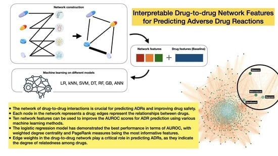
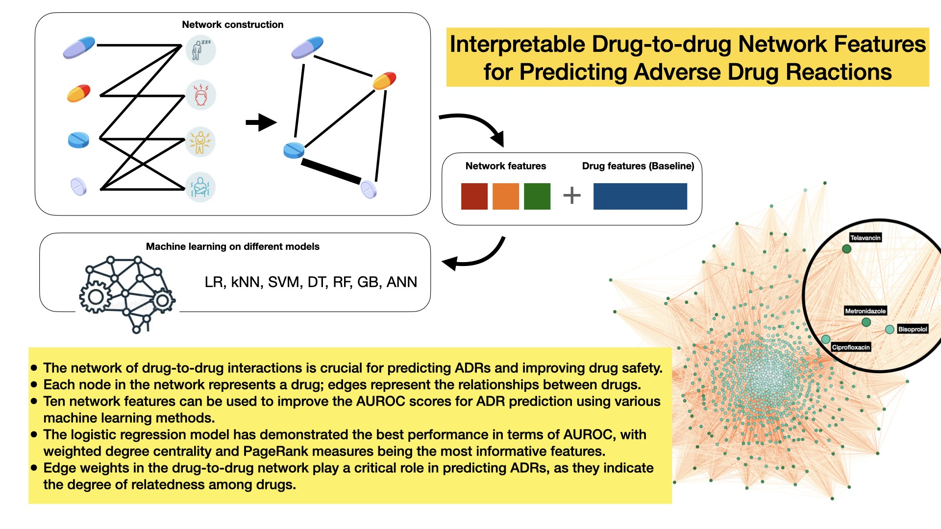
Interpretable Drug-to-Drug Network Features for Predicting Adverse Drug Reactions


Abstract
:
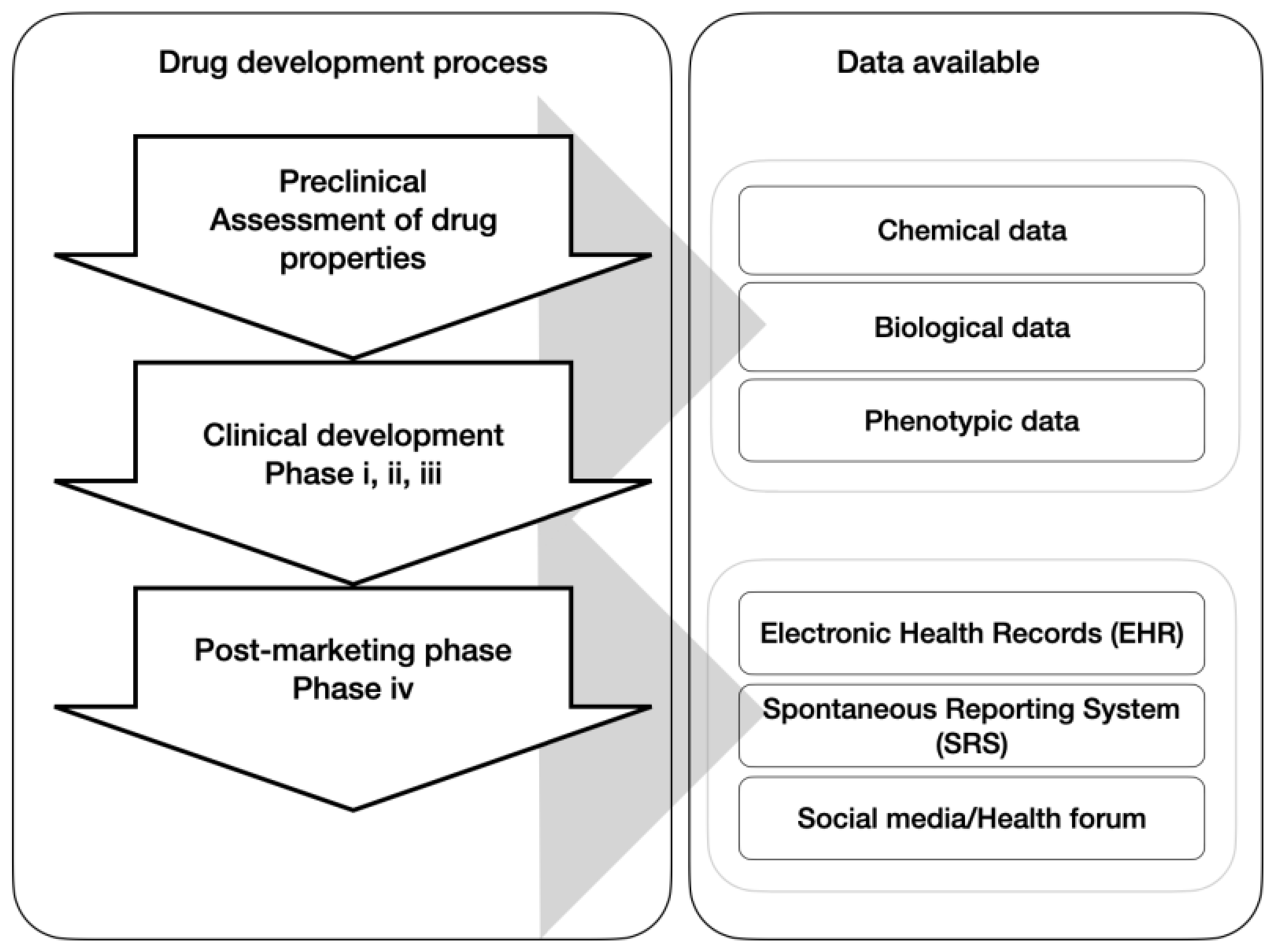
1. Introduction
2. Materials and Methods
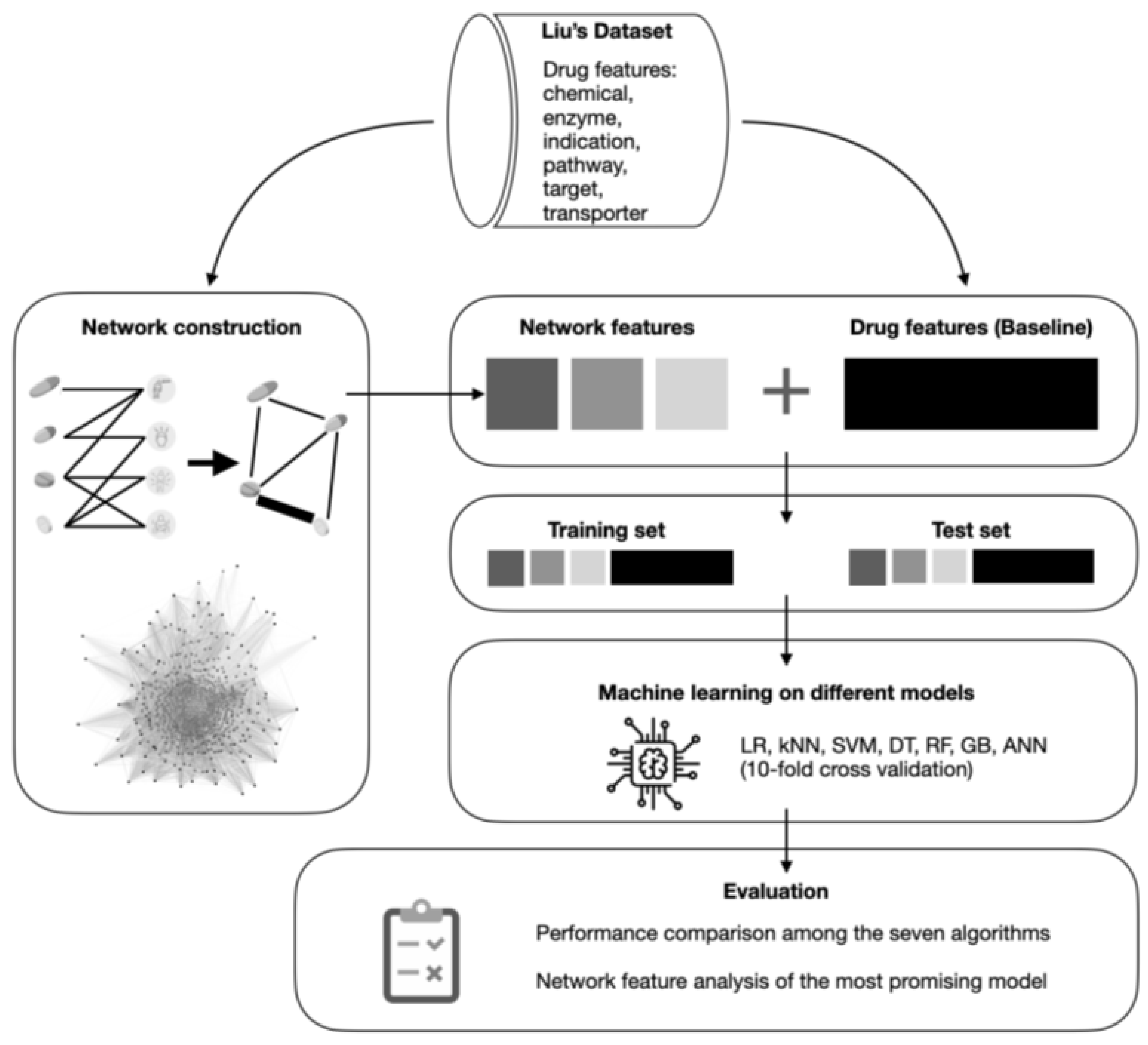
2.1. Dataset Description and Pre-Processing
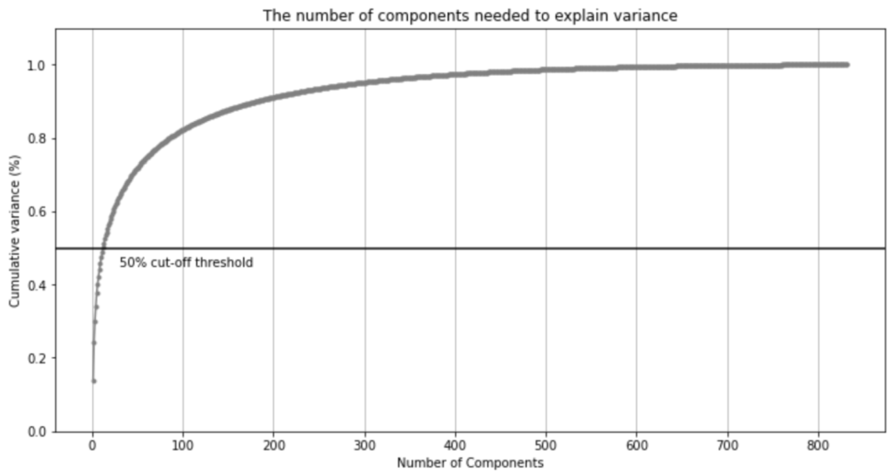
2.2. PCA Applied to One-Hot Vectors of Drugs’ Features
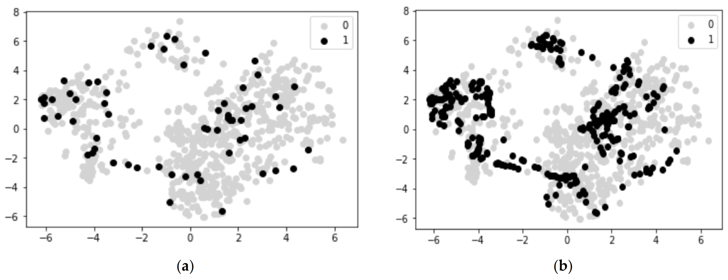
2.3. SMOTE for Imbalanced Data
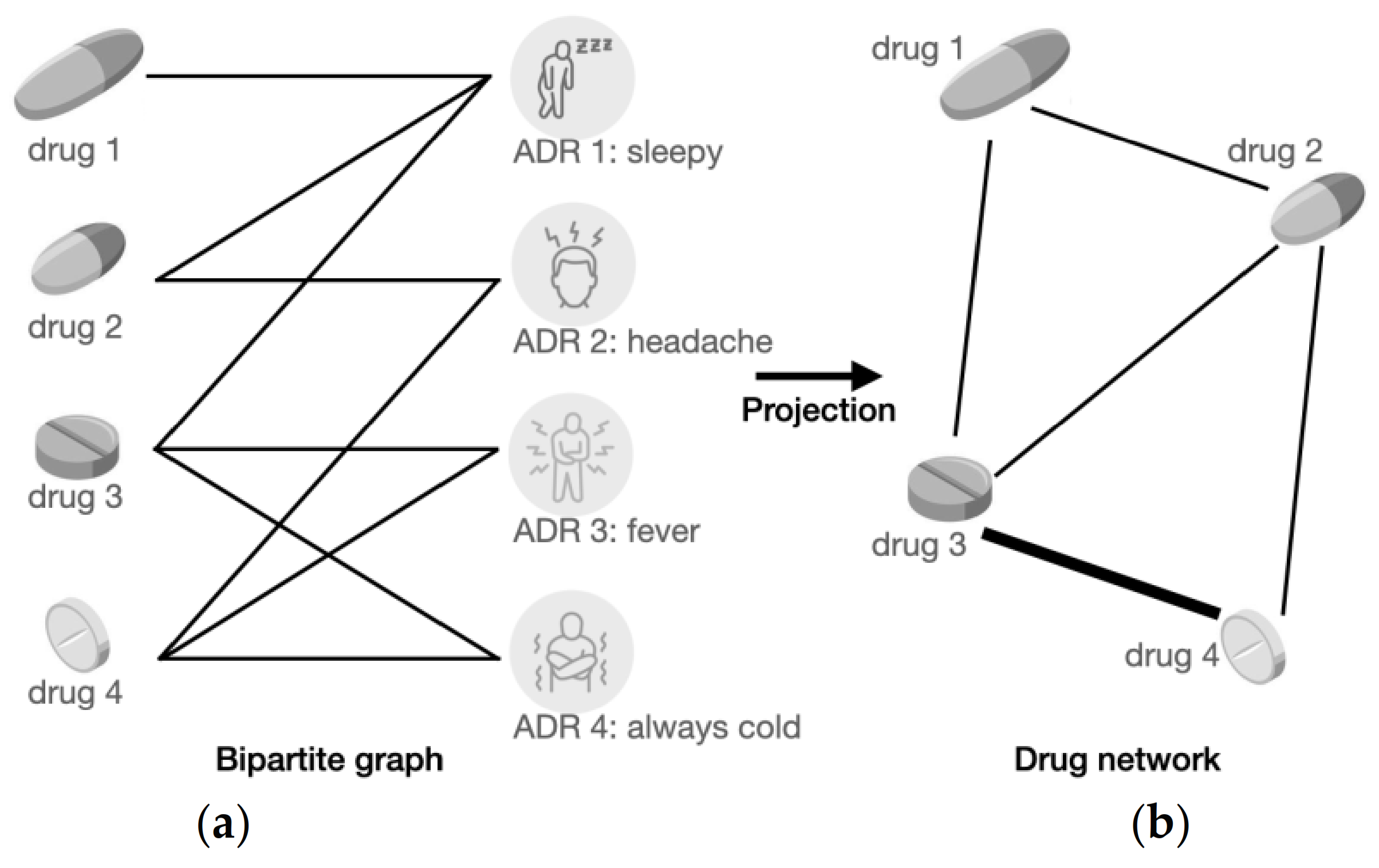
2.4. Drugs Network Construction
2.4.1. Bipartite Graph Construction
2.4.2. Bipartite Graph Projection
2.5. Network Features
2.6. Machine Learning Pipeline and Implementations
| Algorithm 1: Pseudocode of the experiment design |
| Begin For each ADR do Count how many drugs are associated with it and save it in variable N If N < 15 do Move to the next one End if If N >= 15 do If positive cases/negative cases < 0.4 do Apply SMOTE End if Apply learning algorithm and 10-fold cross-validation End if Calculate the average metrics for each algorithm End |
3. Results
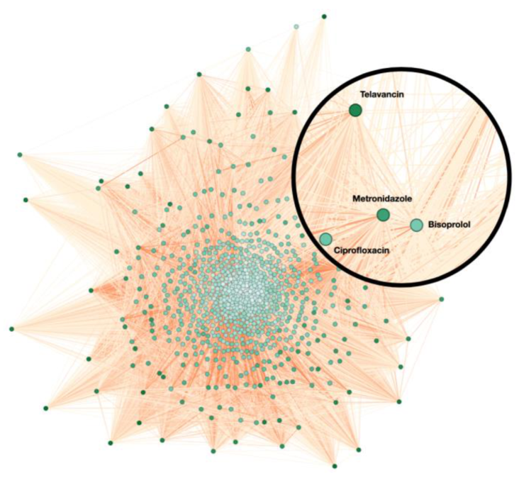
3.1. Network Overview
3.2. Performance of the Proposed Methods Compared to the Baseline
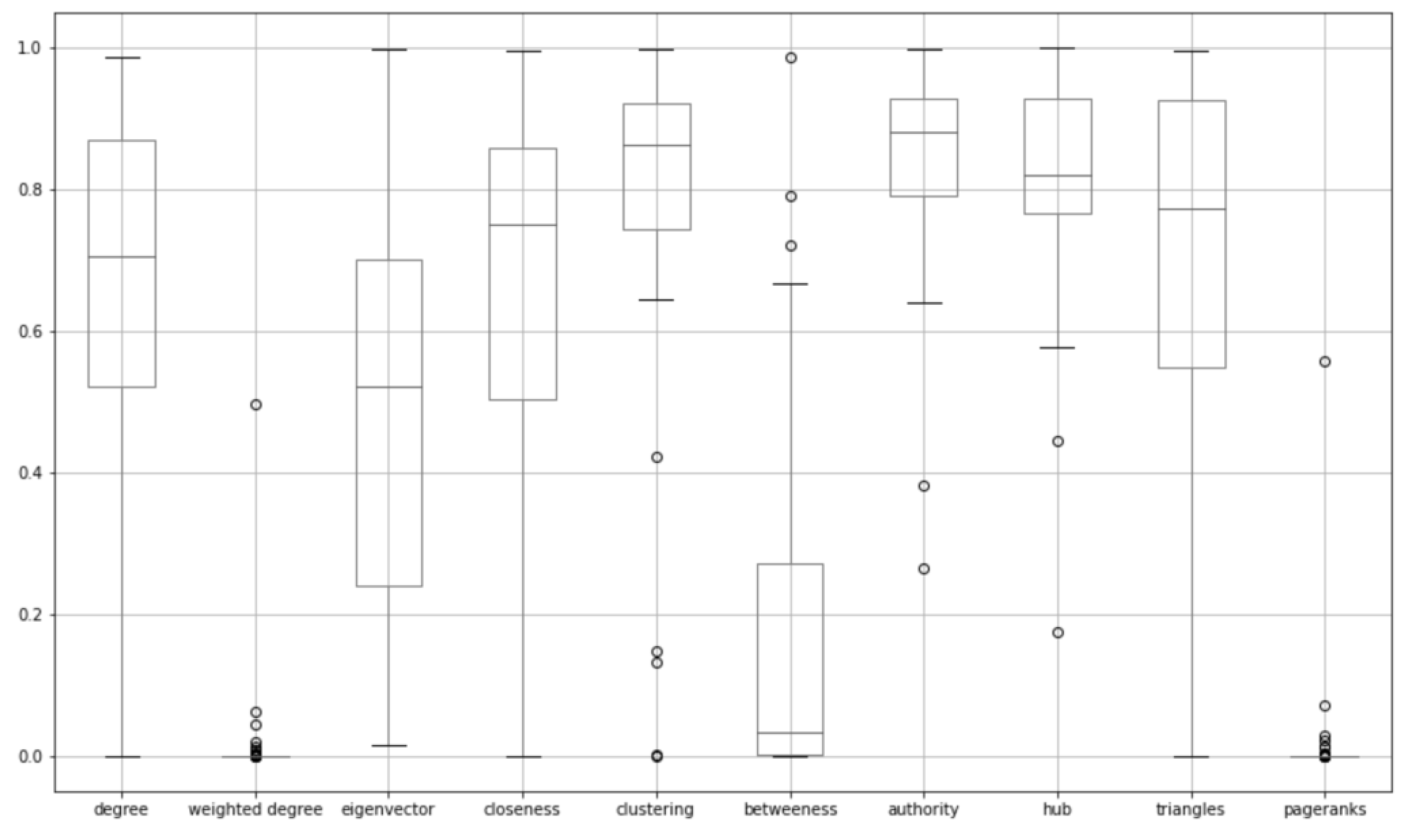
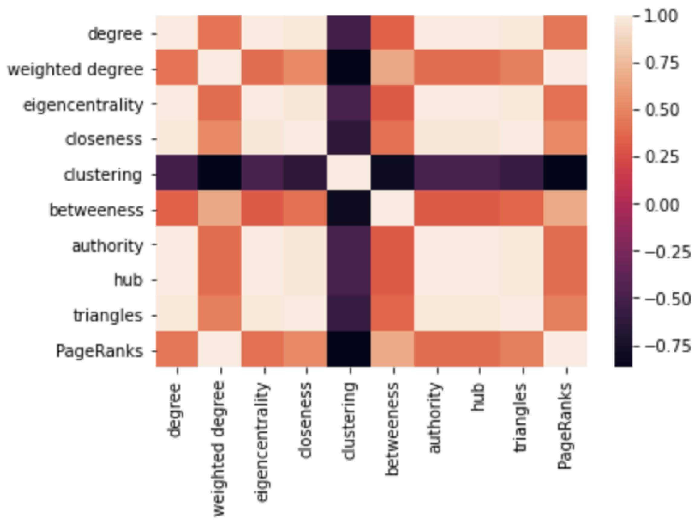
3.2.1. Network Features Assessment
3.2.2. ADRs Prediction Ranks from Logistic Regression Model
3.2.3. Feature Importance
4. Discussion
5. Conclusions
Supplementary Materials
Author Contributions
Funding
Institutional Review Board Statement
Informed Consent Statement
Data Availability Statement
Conflicts of Interest
References
- World Health Organization. The Importance of Pharmacovigilance; World Health Organization: Geneva, Switzerland, 2002. [Google Scholar]
- Sahu, R.K.; Yadav, R.; Prasad, P.; Roy, A.; Chandrakar, S. Adverse drug reactions monitoring: Prospects and impending challenges for pharmacovigilance. Springerplus 2014, 3, 695. [Google Scholar] [CrossRef] [Green Version]
- Berlin, J.A.; Glasser, S.C.; Ellenberg, S.S. Adverse event detection in drug development: Recommendations and obligations beyond phase 3. Am. J. Public Health 2008, 98, 1366–1371. [Google Scholar] [CrossRef] [PubMed]
- Norén, G.N.; Edwards, I.R. Modern methods of pharmacovigilance: Detecting adverse effects of drugs. Clin. Med. 2009, 9, 486. [Google Scholar] [CrossRef] [PubMed]
- Lazarou, J.; Pomeranz, B.H.; Corey, P.N. Incidence of adverse drug reactions in hospitalized patients: A meta-analysis of prospective studies. JAMA 1998, 279, 1200–1205. [Google Scholar] [CrossRef] [PubMed]
- Miguel, A.; Azevedo, L.F.; Araújo, M.; Pereira, A.C. Frequency of adverse drug reactions in hospitalized patients: A systematic review and meta-analysis. Pharmacoepidemiol. Drug Saf. 2012, 21, 1139–1154. [Google Scholar] [CrossRef]
- Hazell, L.; Shakir, S.A.W. Under-Reporting of Adverse Drug Reactions. Drug Saf. 2006, 29, 385–396. [Google Scholar] [CrossRef]
- Hochberg, A.M.; Hauben, M. Time-to-signal comparison for drug safety data-mining algorithms vs. traditional signaling criteria. Clin. Pharmacol. Ther. 2009, 85, 600–606. [Google Scholar] [CrossRef]
- Nguyen, D.A.; Nguyen, C.H.; Mamitsuka, H. A survey on adverse drug reaction studies: Data, tasks and machine learning methods. Brief. Bioinform. 2021, 22, 164–177. [Google Scholar] [CrossRef]
- Kanehisa, M.; Goto, S. KEGG: Kyoto Encyclopedia of Genes and Genomes. Nucleic. Acids Res. 2000, 28, 27–30. [Google Scholar] [CrossRef]
- Liu, M.; Wu, Y.; Chen, Y.; Sun, J.; Zhao, Z.; Chen, X.-W.; Matheny, M.E.; Xu, H. Large-scale prediction of adverse drug reactions using chemical, biological, and phenotypic properties of drugs. J. Am. Med. Inform. Assoc. 2012, 19, e28–e35. [Google Scholar] [CrossRef] [Green Version]
- Belleau, F.; Nolin, M.-A.; Tourigny, N.; Rigault, P.; Morissette, J. Bio2RDF: Towards a mashup to build bioinformatics knowledge systems. J. Biomed. Inform. 2008, 41, 706–716. [Google Scholar] [CrossRef]
- Cao, D.S.; Xiao, N.; Li, Y.J.; Zeng, W.B.; Liang, Y.Z.; Lu, A.P.; Xu, Q.S.; Chen, A. Integrating multiple evidence sources to predict adverse drug reactions based on a systems pharmacology model. CPT Pharmacomet. Syst. Pharmacol. 2015, 4, 498–506. [Google Scholar] [CrossRef] [Green Version]
- Liang, H.; Chen, L.; Zhao, X.; Zhang, X. Prediction of Drug Side Effects with a Refined Negative Sample Selection Strategy. Comput. Math Methods Med. 2020, 2020, 1573543. [Google Scholar] [CrossRef]
- Song, D.; Chen, Y.; Min, Q.; Sun, Q.; Ye, K.; Zhou, C.; Yuan, S.; Sun, Z.; Liao, J. Similarity-based machine learning support vector machine predictor of drug-drug interactions with improved accuracies. J. Clin. Pharm. Ther. 2019, 44, 268–275. [Google Scholar] [CrossRef]
- Lee, C.Y.; Chen, Y. Machine learning on adverse drug reactions for pharmacovigilance. Drug Discov. Today 2019, 24, 1332–1343. [Google Scholar] [CrossRef]
- Hu, B.; Wang, H.; Yu, Z. Drug Side-Effect Prediction Via Random Walk on the Signed Heterogeneous Drug Network. Molecules 2019, 24, 3668. [Google Scholar] [CrossRef] [Green Version]
- Kwak, H.; Lee, M.; Yoon, S.; Chang, J.; Park, S.; Jung, K. Drug-Disease Graph: Predicting Adverse Drug Reaction Signals via Graph Neural Network with Clinical Data. In Proceedings of the Advances in Knowledge Discovery and Data Mining: 24th Pacific-Asia Conference PAKDD 2020, Singapore, 11–14 May 2020; Volume 12085, pp. 633–644. [Google Scholar]
- Zitnik, M.; Agrawal, M.; Leskovec, J. Modeling polypharmacy side effects with graph convolutional networks. Bioinformatics 2018, 34, i457–i466. [Google Scholar] [CrossRef] [Green Version]
- Zhou, F.; Uddin, S. How could a weighted drug-drug network help improve adverse drug reaction predictions? Machine learning reveals the importance of edge weights. In Proceedings of the Australasian Computer Science Week Multiconference, Melbourne, Australia,, 31 January–3 February 2023; 2023. [Google Scholar]
- Chawla, N.V.; Bowyer, K.W.; Hall, L.O.; Kegelmeyer, W.P. SMOTE: Synthetic minority over-sampling technique. J. Artif. Intell. Res. 2002, 16, 321–357. [Google Scholar] [CrossRef]
- Bastian, M.; Heymann, S.; Jacomy, M. Gephi: An open source software for exploring and manipulating networks. In Proceedings of the 3rd International AAAI Conference on Weblogs and Social Media, San Jose, CA, USA, 17–20 May 2009. [Google Scholar]
- Blondel, V.D.; Guillaume, J.-L.; Lambiotte, R.; Lefebvre, E. Fast unfolding of communities in large networks. J. Stat.Mech. Theory Exp. 2008, 2008, P10008. [Google Scholar] [CrossRef] [Green Version]
- Opsahl, T.; Agneessens, F.; Skvoretz, J. Node centrality in weighted networks: Generalizing degree and shortest paths. Soc. Netw. 2010, 32, 245–251. [Google Scholar] [CrossRef]
- Golbeck, J. Chapter 3—Network Structure and Measures. In Analyzing the Social Web; Golbeck, J., Ed.; Morgan Kaufmann: Boston, MA, USA, 2013; pp. 25–44. [Google Scholar]
- Freeman, L.C. Centrality in social networks conceptual clarification. Soc. Netw. 1978, 1, 215–239. [Google Scholar] [CrossRef] [Green Version]
- Holland, P.W.; Leinhardt, S. Transitivity in structural models of small groups. Comp. Group Stud. 1971, 2, 107–124. [Google Scholar] [CrossRef]
- Barthélemy, M. Betweenness centrality in large complex networks. Eur. Phys. J. B 2004, 38, 163–168. [Google Scholar] [CrossRef]
- Kleinberg, J.M. Authoritative sources in a hyperlinked environment. J. ACM (JACM) 1999, 46, 604–632. [Google Scholar] [CrossRef] [Green Version]
- Brinkmeier, M. PageRank revisited. ACM Trans. Internet Technol. 2006, 6, 282–301. [Google Scholar] [CrossRef]
- Song, Y.-Y.; Ying, L. Decision tree methods: Applications for classification and prediction. Shanghai Arch. Psychiatry 2015, 27, 130. [Google Scholar]
- Fawagreh, K.; Gaber, M.M.; Elyan, E. Random forests: From early developments to recent advancements. Syst. Sci. Control. Eng. 2014, 2, 602–609. [Google Scholar] [CrossRef] [Green Version]
- Chen, T.; Guestrin, C. Xgboost: A scalable tree boosting system. In Proceedings of the 22nd Acm Sigkdd International Conference on Knowledge Discovery and Data Mining, San Francisco, CA, USA, 13–17 August 2016; pp. 785–794. [Google Scholar]
- Cortes, C.; Vapnik, V. Support-vector networks. Mach. Learn. 1995, 20, 273–297. [Google Scholar] [CrossRef]
- Cover, T.; Hart, P. Nearest neighbor pattern classification. IEEE Trans. Inf. Theory 1967, 13, 21–27. [Google Scholar] [CrossRef] [Green Version]
- Wang, S.-C. Artificial Neural Network. In Interdisciplinary Computing in Java Programming; Wang, S.-C., Ed.; Springer: Boston, MA, USA, 2003; pp. 81–100. [Google Scholar]
- Fawcett, T. An introduction to ROC analysis. Pattern Recognit. Lett. 2006, 27, 861–874. [Google Scholar] [CrossRef]
- Sundaran, S.; Udayan, A.; Hareendranath, K.; Eliyas, B.; Ganesan, B.; Hassan, A.; Subash, R.; Palakkal, V.; Salahudeen, M.S. Study on the Classification, Causality, Preventability and Severity of Adverse Drug Reaction Using Spontaneous Reporting System in Hospitalized Patients. Pharmacy 2018, 6, 108. [Google Scholar] [CrossRef] [Green Version]


| Feature Types | Sources | Number of Features |
|---|---|---|
| Chemical | KEGG | 811 |
| Enzyme | GeneBank | 111 |
| Indication | SIDER | 869 |
| Pathway | KEGG | 173 |
| Target | GeneBank | 786 |
| Transporter | GeneBank | 72 |
| Properties of the Network | Statistics |
|---|---|
| Node count | 832 |
| Edge count | 332,806 |
| Average degree | 800 |
| Network diameter | 2 |
| Average path length | 1.04 |
| Graph density | 0.96 |
| Average clustering coefficient | 0.97 |
| Datasets | Random Forest | Logistic Regression | SVM | kNN | Decision Tree | Gradient Boost Tree | ANN |
|---|---|---|---|---|---|---|---|
| Baseline | 0.618 | 0.595 | 0.608 | 0.593 | 0.542 | 0.595 | 0.670 |
| Baseline + D * | 0.770 | 0.633 | 0.644 | 0.599 | 0.603 | 0.761 | 0.688 |
| Baseline + DW * | 0.802 | 0.814 | 0.811 | 0.727 | 0.623 | 0.787 | 0.813 |
| Baseline + DWE * | 0.803 | 0.815 | 0.813 | 0.727 | 0.621 | 0.786 | 0.813 |
| Baseline + DWEO * | 0.803 | 0.815 | 0.813 | 0.727 | 0.621 | 0.787 | 0.817 |
| Baseline + DWEOC * | 0.805 | 0.819 | 0.816 | 0.735 | 0.622 | 0.790 | 0.816 |
| Baseline + DWEOCB * | 0.805 | 0.819 | 0.816 | 0.737 | 0.623 | 0.792 | 0.816 |
| Baseline + DWEOCBA * | 0.805 | 0.819 | 0.816 | 0.737 | 0.623 | 0.792 | 0.817 |
| Baseline + DWEOCBAH * | 0.804 | 0.819 | 0.816 | 0.736 | 0.623 | 0.792 | 0.817 |
| Baseline + DWEOCBAH T * | 0.804 | 0.819 | 0.817 | 0.737 | 0.622 | 0.792 | 0.817 |
| Baseline + DWEOCBAHTP * | 0.806 | 0.821 | 0.819 | 0.743 | 0.622 | 0.791 | 0.818 |
| ADR id | ADR Name | AUROC without Network Features | AUROC with Network Features | Improvement | Accuracy with Network Features |
|---|---|---|---|---|---|
| 961 [C0085624] | Burning sensation | 0.490 | 0.998 | 0.508 | 0.990 |
| 951 [C0085583] | Choreoathetosis | 0.740 | 0.966 | 0.226 | 0.951 |
| 564 [C0026113] | Miliaria | 0.936 | 0.958 | 0.022 | 0.959 |
| 371 [C0018991] | Hemiplegia | 0.568 | 0.947 | 0.379 | 0.919 |
| 1078 [C0162316] | Iron deficiency anemia | 0.646 | 0.947 | 0.301 | 0.927 |
| 753 [C0034186] | Pyelonephritis | 0.494 | 0.943 | 0.449 | 0.918 |
| 226 [C0012813] | Diverticulitis | 0.813 | 0.941 | 0.128 | 0.929 |
| 645 [C0029878] | Otitis externa | 0.506 | 0.939 | 0.433 | 0.922 |
| 204 [C0011334] | Tooth caries | 0.519 | 0.937 | 0.418 | 0.921 |
| 541 [C0024894] | Mastitis | 0.508 | 0.932 | 0.424 | 0.916 |
| Network Features | Mean of p-Values | Standard Deviation of p-Values |
|---|---|---|
| Degree | 0.673447 | 0.252389 |
| Weighted degree | 0.010291 | 0.063076 |
| Eigenvector | 0.511627 | 0.287661 |
| Closeness | 0.654633 | 0.274280 |
| Clustering coefficient | 0.793905 | 0.219335 |
| Betweenness | 0.190212 | 0.260536 |
| Authority | 0.849929 | 0.132538 |
| Hub | 0.823477 | 0.140945 |
| Triangles | 0.711467 | 0.264627 |
| Weighted PageRanks | 0.011244 | 0.070466 |
Disclaimer/Publisher’s Note: The statements, opinions and data contained in all publications are solely those of the individual author(s) and contributor(s) and not of MDPI and/or the editor(s). MDPI and/or the editor(s) disclaim responsibility for any injury to people or property resulting from any ideas, methods, instructions or products referred to in the content. |
© 2023 by the authors. Licensee MDPI, Basel, Switzerland. This article is an open access article distributed under the terms and conditions of the Creative Commons Attribution (CC BY) license (https://creativecommons.org/licenses/by/4.0/).
Share and Cite
Zhou, F.; Uddin, S. Interpretable Drug-to-Drug Network Features for Predicting Adverse Drug Reactions. Healthcare 2023, 11, 610. https://doi.org/10.3390/healthcare11040610
Zhou F, Uddin S. Interpretable Drug-to-Drug Network Features for Predicting Adverse Drug Reactions. Healthcare. 2023; 11(4):610. https://doi.org/10.3390/healthcare11040610
Chicago/Turabian StyleZhou, Fangyu, and Shahadat Uddin. 2023. "Interpretable Drug-to-Drug Network Features for Predicting Adverse Drug Reactions" Healthcare 11, no. 4: 610. https://doi.org/10.3390/healthcare11040610