
Intelligent Diagnostic Prediction and Classification Models for Detection of Kidney Disease

 ,
,  , ,
, ,
Abstract
:1. Introduction
Chronic Kidney Disease
- Review the existing approaches for the detection of kidney disease.
- Determine the best feature by applying various feature selection techniques.
- Build various prediction models on a kidney dataset using different machine learning algorithms and analyze their accuracy in the detection of kidney disease.
2. Related Works
3. Support Vector Machine
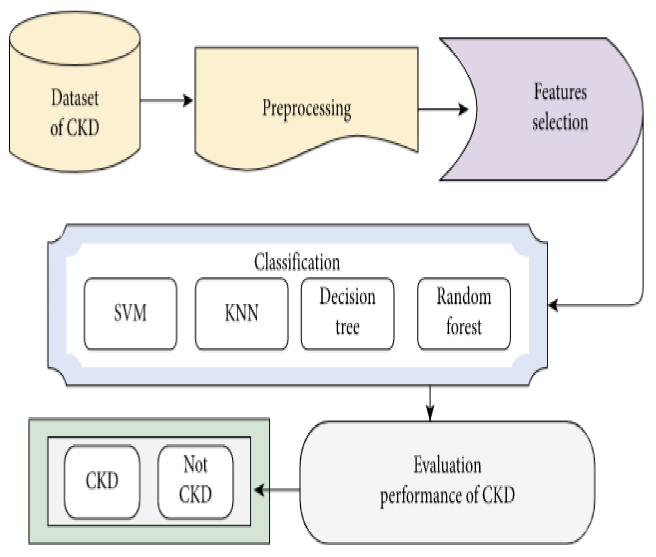
4. Materials and Methods
4.1. Kidney Disease Dataset
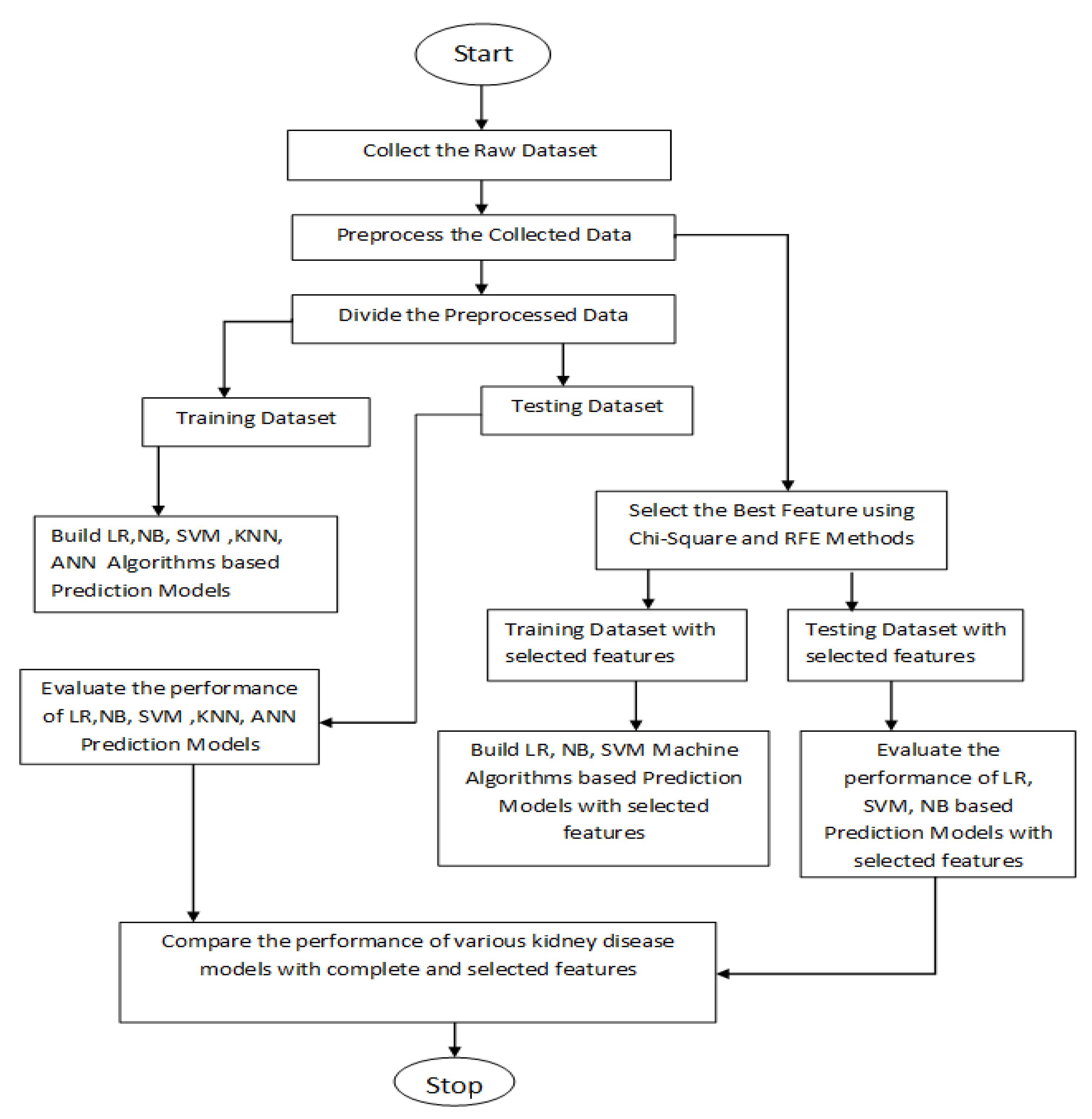
4.2. Proposed Algorithm
- In the ‘rbc’ and ‘pc’ columns, ‘normal’ and ‘abnormal’ nominal values are replaced with 1 and 0, respectively.
- In the ‘pcc’ and ‘ba’ columns, the ‘present’ and ‘nonpresent’ values are replaced with 1 and 0, respectively.
- In the ‘htn’, ‘pe’, ’ane’, ‘dm’, and ‘cad’ columns, the values ‘yes’ and ‘no’ are replaced with 1 and 0, respectively.
- Finally, in the ‘appet’ column, ‘good’ and ‘poor’ are replaced with 1 and 0, respectively.
5. Results and Analysis
5.1. Performance Measures
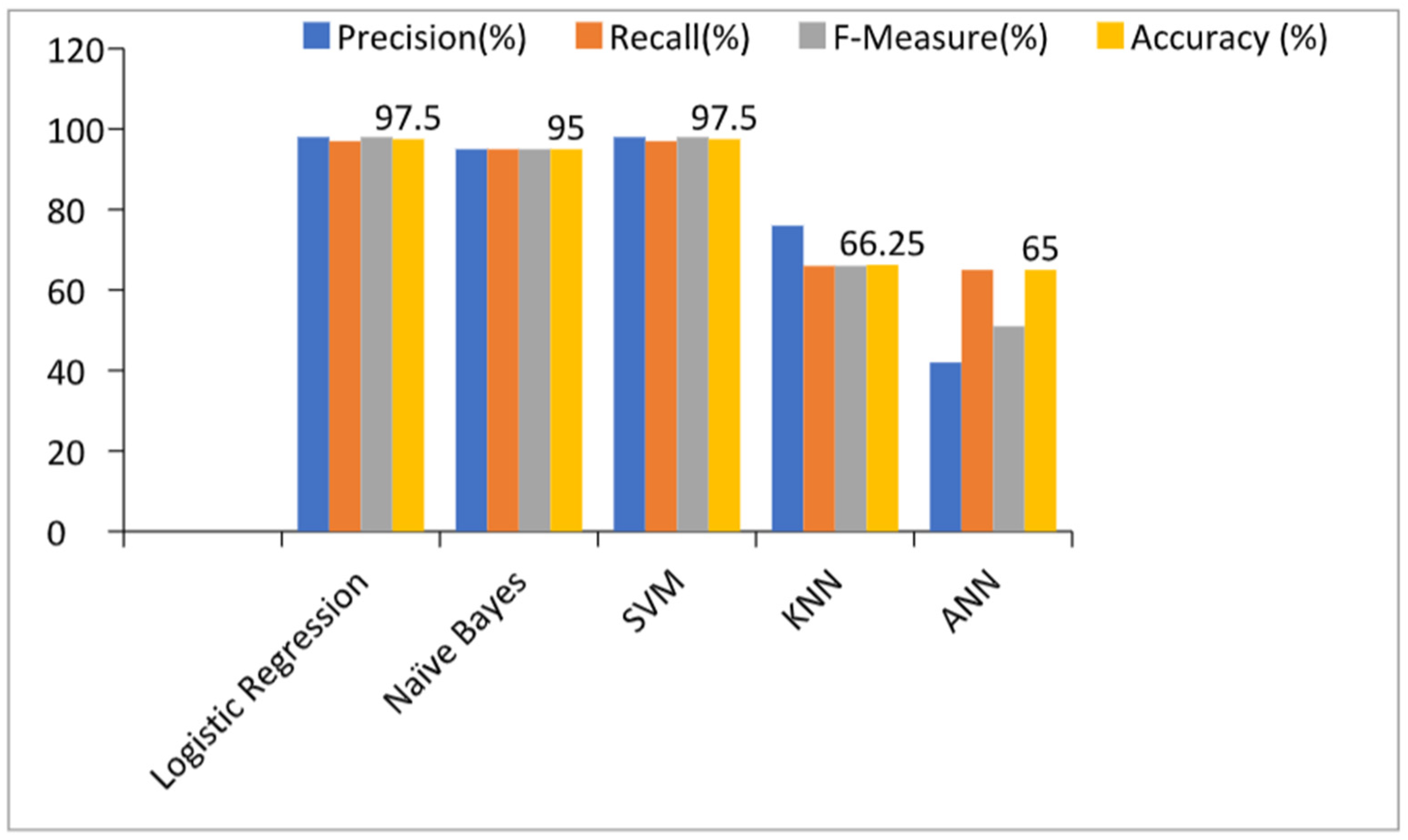
5.2. Prediction Models with All Features
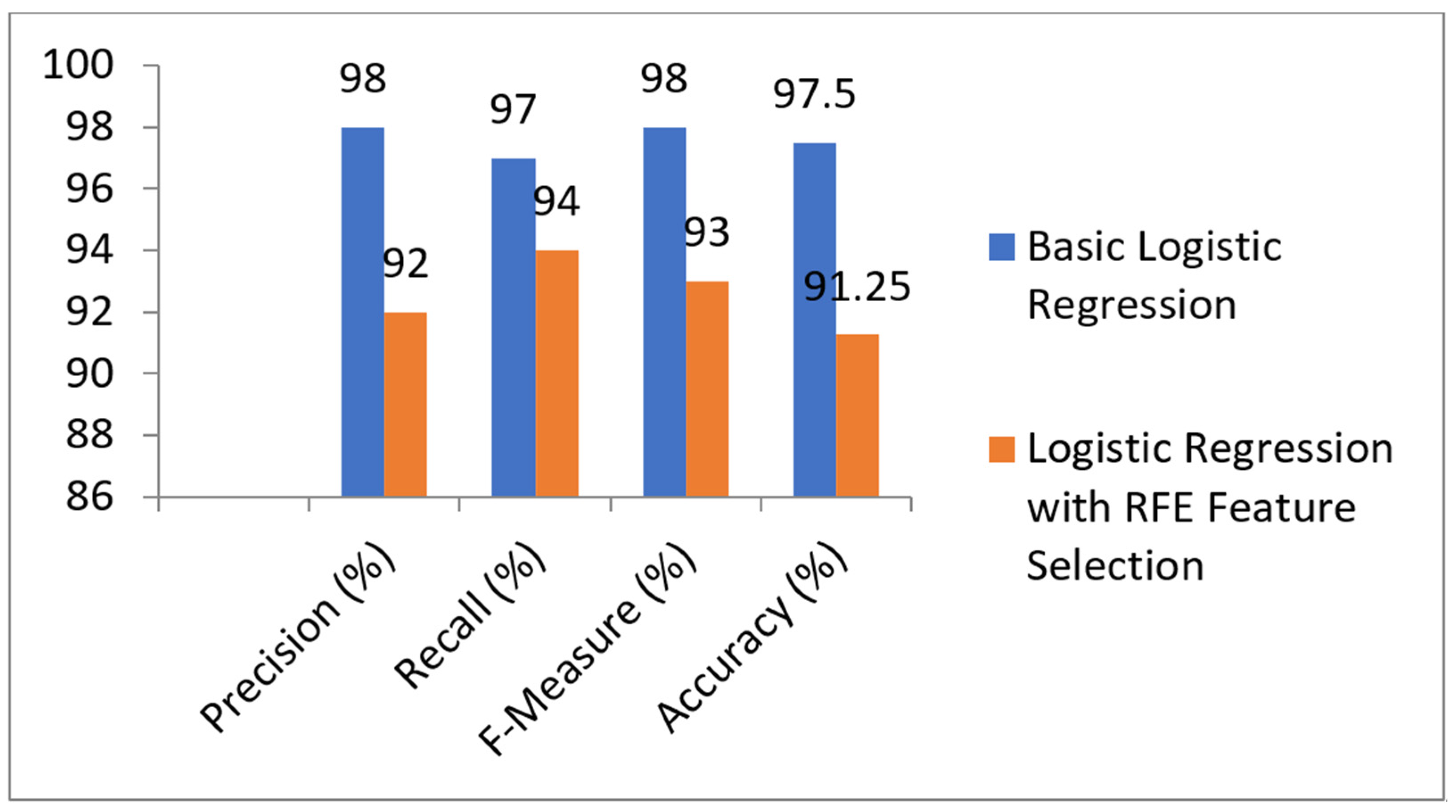
5.3. Prediction Models with RFE Feature Selection Technique
5.4. Performance of Prediction Models with Chi-Square Feature Selection
5.5. Comparison of Models with and without Feature Selection Technique
6. Conclusions and Future Work
Author Contributions
Funding
Institutional Review Board Statement
Informed Consent Statement
Data Availability Statement
Acknowledgments
Conflicts of Interest
References
- Aljaaf, A.J. Early Prediction of Chronic Kidney Disease Using Machine Learning Supported by Predictive Analytics. In Proceedings of the IEEE Congress on Evolutionary Computation (CEC), Wellington, New Zealand, 8–13 July 2018. [Google Scholar]
- Nishanth, A.; Thiruvaran, T. Identifying Important Attributes for Early Detection of Chronic Kidney Disease. IEEE Rev. Biomed. Eng. 2018, 11, 208–216. [Google Scholar] [CrossRef] [PubMed]
- Ogunleye, A.; Wang, Q.-G. XGBoost Model for Chronic Kidney Disease Diagnosis. IEEE/ACM Trans. Comput. Biol. Bioinform. 2020, 17, 2131–2140. [Google Scholar] [CrossRef] [PubMed]
- Aqlan, F.; Markle, R.; Shamsan, A. Data Mining for Chronic Kidney Disease Prediction. In Proceedings of the 67th Annual Conference and Expo of the Institute of Industrial Engineers, Pittsburgh, PA, USA, 20–23 May 2017. [Google Scholar]
- Borisagar, N.; Barad, D.; Raval, P. Chronic Kidney Disease Prediction Using Back Propagation Neural Network Algorithm. In Proceedings of the International Conference on Communication and Networks, Ahmedabad, India, 19–20 February 2017; pp. 295–303. [Google Scholar]
- Boukenze, B.; Haqiq, A.; Mousannif, H. Predicting Chronic Kidney Failure Disease Using Data Mining Techniques. In Advances in Ubiquitous Networking; El-Azouzi, R., Menasche, D.S., Sabir, E., De Pellegrini, F., Benjillali, M., Eds.; Springer: New York, NY, USA, 2018; Volume 2, pp. 701–712. [Google Scholar]
- Polat, H.; Mehr, H.D.; Cetin, A. Diagnosis of chronic kidney disease based on support vector machine by feature selection methods. J. Med. Syst. 2017, 41, 55. [Google Scholar] [CrossRef] [PubMed]
- Panwong, P.; Iam-On, N. Predicting transitional interval of kidney disease stages 3 to 5 using data mining method. In Proceedings of the 2016 Second Asian Conference on Defence Technology (ACDT), Chiang Mai, Thailand, 21–23 January 2016; pp. 145–150. [Google Scholar] [CrossRef]
- Dulhare, U.N.; Ayesha, M. Extraction of action rules for chronic kidney disease using Naïve bayes classifier. In Proceedings of the 2016 IEEE International Conference on Computational Intelligence and Computing Research (ICCIC), Chennai, India, 15–17 December 2016; pp. 1–5. [Google Scholar] [CrossRef]
- Vasquez-Morales, G.R.; Martinez-Monterrubio, S.M.; Moreno-Ger, P.; Recio-Garcia, J.A. Explainable Prediction of Chronic Renal Disease in the Colombian Population Using Neural Networks and Case-Based Reasoning. IEEE Access 2019, 7, 152900–152910. [Google Scholar] [CrossRef]
- Makino, M.; Yoshimoto, R.; Ono, M.; Itoko, T.; Katsuki, T.; Koseki, A.; Kudo, M.; Haida, K.; Kuroda, J.; Yanagiya, R.; et al. Artificial intelligence predicts the progression of diabetic kidney disease using big data machine learning. Sci. Rep. 2019, 9, 11862. [Google Scholar] [CrossRef] [Green Version]
- Ren, Y.; Fei, H.; Liang, X.; Ji, D.; Cheng, M. A hybrid neural network model for predicting kidney disease in hypertension patients based on electronic health records. BMC Med. Inf. Decis. Mak. 2019, 19, 131–138. [Google Scholar] [CrossRef]
- Ma, F.; Sun, T.; Liu, L.; Jing, H. Detection and diagnosis of chronic kidney disease using deep learning-based heterogeneous modified artificial neural network. Future Gener. Comput. Syst. 2020, 111, 17–26. [Google Scholar] [CrossRef]
- Almansour, N.; Syed, H.F.; Khayat, N.R.; Altheeb, R.K.; Juri, R.E.; Alhiyafi, J.; Alrashed, S.; Olatunji, S.O. Neural network and support vector machine for the prediction of chronic kidney disease: A comparative study. Comput. Biol. Med. 2019, 109, 101–111. [Google Scholar] [CrossRef]
- Qin, J.; Chen, L.; Liu, Y.; Liu, C.; Feng, C.; Chen, B. A Machine Learning Methodology for Diagnosing Chronic Kidney Disease. IEEE Access 2019, 8, 20991–21002. [Google Scholar] [CrossRef]
- Segal, Z.; Kalifa, D.; Radinsky, K.; Ehrenberg, B.; Elad, G.; Maor, G.; Lewis, M.; Tibi, M.; Korn, L.; Koren, G. Machine learning algorithm for early detection of end-stage renal disease. BMC Nephrol. 2020, 21, 518. [Google Scholar] [CrossRef]
- Khamparia, A.; Saini, G.; Pandey, B.; Tiwari, S.; Gupta, D.; Khanna, A. KDSAE: Chronic kidney disease classification with multimedia data learning using deep stacked autoencoder network. Multimed. Tools Appl. 2020, 79, 35425–35440. [Google Scholar] [CrossRef]
- Dua, D.; Graff, C. UCI Machine Learning Repository. 2019. Available online: http://archive.ics.uci.edu/ml (accessed on 6 December 2021).
- Ebiaredoh-Mienye, S.A.; Esenogho, E.; Swart, T.G. Integrating Enhanced Sparse Autoencoder-Based Artificial Neural Network Technique and Softmax Regression for Medical Diagnosis. Electronics 2020, 9, 1963. [Google Scholar] [CrossRef]
- Pang, Z.; Zhu, D.; Chen, D.; Li, L.; Shao, Y. A Computer-Aided Diagnosis System for Dynamic Contrast-Enhanced MR Images Based on Level Set Segmentation and ReliefF Feature Selection. Comput. Math. Methods Med. 2015, 2015, 450531. [Google Scholar] [CrossRef] [PubMed]
- Chen, G.; Ding, C.; Li, Y.; Hu, X.; Li, X.; Ren, L.; Ding, X.; Tian, P.; Xue, W. Prediction of Chronic Kidney Disease Using Adaptive Hybridized Deep Convolutional Neural Network on the Internet of Medical Things Platform. IEEE Access 2020, 8, 100497–100508. [Google Scholar] [CrossRef]
- Khan, B.; Naseem, R.; Muhammad, F.; Abbas, G.; Kim, S. An Empirical Evaluation of Machine Learning Techniques for Chronic Kidney Disease Prophecy. IEEE Access 2020, 8, 55012–55022. [Google Scholar] [CrossRef]
- Tabassum, M.; Bai, B.G.; Majumdar, J. Analysis and Prediction of Chronic Kidney Disease using Data Mining Techniques. Int. J. Eng. Res. Comput. Sci. Eng. 2018, 4, 25–31. [Google Scholar]
- Padmanaban, K.R.A.; Parthiban, G. Applying Machine Learning Techniques for Predicting the Risk of Chronic Kidney Disease. Indian J. Sci. Technol. 2016, 9. [Google Scholar] [CrossRef]
- Sharma, S.; Sharma, V.; Sharma, A. Performance Based Evaluation of Various Machine Learning Classification Techniques for Chronic Kidney Disease Diagnosis. Int. J. Mod. Comput. Sci. 2018, 4, 11–15. [Google Scholar]
- Devishri, P.; Ragin, S.; Anisha, O.R. Comparative Study of Classification Algorithms in Chronic Kidney Disease. Int. J. Recent Technol. Eng. 2019, 8, 180–184. [Google Scholar]
- Drall, S.; Drall, G.S.; Singh, S. Chronic Kidney Disease Prediction Using Machine Learning: A New Approach. Int. J. Manag. 2018, 8, 278. [Google Scholar]
- Dang, B.V.; Taylor, R.A.; Charlton, A.J.; Le-Clech, P.; Barber, T.J. Toward Portable Artificial Kidneys: The Role of Advanced Microfluidics and Membrane Technologies in Implantable Systems. IEEE Rev. Biomed. Eng. 2020, 13, 261–279. [Google Scholar] [CrossRef] [PubMed]
- Cheng, L.C.; Hu, Y.H.; Chiou, S.H. Applying the Temporal Abstraction Technique to the Prediction of Chronic Kidney Disease Progression. J. Med. Syst. 2019, 41, 85. [Google Scholar] [CrossRef] [PubMed]
- Hodneland, E. In Vivo Detection of Chronic Kidney Disease Using Tissue Deformation Fields from Dynamic MR Imaging. IEEE Trans. Biomed. Eng. 2019, 66, 1779–1790. [Google Scholar] [CrossRef] [PubMed]
- Marsh, J.N.; Matlock, M.K.; Kudose, S.; Liu, T.-C.; Stappenbeck, T.S.; Gaut, J.P.; Swamidass, S.J. Deep Learning Global Glomerulosclerosis in Transplant Kidney Frozen Sections. IEEE Trans. Med. Imaging 2018, 37, 2718–2728. [Google Scholar] [CrossRef] [PubMed]
- Antony, L.; Azam, S.; Ignatious, E.; Quadir, R.; Beeravolu, A.R.; Jonkman, M.; De Boer, F. A Comprehensive Unsupervised Framework for Chronic Kidney Disease Prediction. IEEE Access 2021, 9, 126481–126501. [Google Scholar] [CrossRef]
- Hossain, M.; Detwiler, R.K.; Chang, E.H.; Caughey, M.C.; Fisher, M.W.; Nichols, T.C.; Merricks, E.P.; Raymer, R.A.; Whitford, M.; Bellinger, D.A.; et al. Mechanical Anisotropy Assessment in Kidney Cortex Using ARFI Peak Displacement: Preclinical Validation and Pilot In Vivo Clinical Results in Kidney Allografts. IEEE Trans. Ultrason. Ferroelectr. Freq. Control 2018, 66, 551–562. [Google Scholar] [CrossRef] [PubMed]
- Hussain, M.A.; Hamarneh, G.; Garbi, R. Cascaded Localization Regression Neural Nets for Kidney Localization and Segmentation-free Volume Estimation. IEEE Trans. Med. Imaging 2021, 40, 1555–1567. [Google Scholar] [CrossRef]
- Shehata, M.; Khalifa, F.; Soliman, A.; Ghazal, M.; Taher, F.; El-Ghar, M.A.; Dwyer, A.C.; Gimel’Farb, G.; Keynton, R.S.; El-Baz, A. Computer-Aided Diagnostic System for Early Detection of Acute Renal Transplant Rejection Using Diffusion-Weighted MRI. IEEE Trans. Biomed. Eng. 2018, 66, 539–552. [Google Scholar] [CrossRef]
- Bhaskar, N.; Manikandan, S.M.S. A Deep-Learning-Based System for Automated Sensing of Chronic Kidney Disease. IEEE Sens. Lett. 2019, 3, 1–4. [Google Scholar] [CrossRef]
- Chittora, P.; Chaurasia, S.; Chakrabarti, P.; Kumawat, G.; Chakrabarti, T.; Leonowicz, Z.; Jasinski, M.; Jasinski, L.; Gono, R.; Jasinska, E.; et al. Prediction of Chronic Kidney Disease—A Machine Learning Perspective. IEEE Access 2021, 9, 17312–17334. [Google Scholar] [CrossRef]
- Zollner, F.G.; Kocinski, M.; Hansen, L.; Golla, A.-K.; Trbalic, A.S.; Lundervold, A.; Materka, A.; Rogelj, P. Kidney Segmentation in Renal Magnetic Resonance Imaging—Current Status and Prospects. IEEE Access 2021, 9, 71577–71605. [Google Scholar] [CrossRef]


| Sr. No. | Author | Year | Machine Learning Algorithms and Accuracy (%) |
|---|---|---|---|
| 1. | A. J. Aljaaf et al. [1] | 2018 | Naïve Bayes: 83.4%, J48: 86.23% |
| 2. | N. Borisagar, D. Barad, and P. Raval [5] | 2017 | ANN: 99.5 |
| 3. | B. Boukenze, A. Haqiq, and H. Mousannif [6] | 2018 | SVM: 63.5%, LR: 64.0, C4.5: 63%, KNN: 55.15% |
| 4. | H. Polat, H. D. Mehr and A. Cetin [7] | 2019 | SVM: 97.5% |
| 5. | P. Panwong and N. Iam-On [8] | 2016 | KNN: 86.32%, naïve Bayes: 60.46%, ANN: 83.24%, RF: 86.60%, J48: 79.52% |
| 6. | Makino et al. [11] | 2019 | KNN, Naïve Bayes + LDA + random subspace + Tree-based decision: 94% |
| 7. | Ren et al. [12] | 2019 | SVM + ReliefF: 92.7% |
| 8. | Ma F. et al. [13] | 2019 | Fisher discriminatory analysis and SVM: 96.7% |
| 9. | Almansour and colleagues [14] | 2020 | KNN and SVM: 99% |
| 10. | J. Qin and colleagues [15] | 2019 | SVM, KNN, and naïve Bayes decision tree: 99.7% |
| 11. | Z. Segal and colleagues [16] | 2019 | SVM, KNN, and decision tree: 99.1% |
| 12. | Khamparia et al. [17] | 2020 | Logistic regression, KNN, SVM, random forest, naive Bayes, and ANN: 99.7% |
| 13. | Ebiaredoh-Mienye Sarah A. et al. [18] | 2017 | SVM 98.5% |
| 14. | Zhiyong Pang et al. [19] | 2020 | Softmax regression 98% |
| 15. | Tabassum, Mamatha et al. [23] | 2017 | DT: 85%, RF: 85% |
| 16. | K. R. A. Padmanaban and G. Parthiban [24] | 2016 | DT: 91%, naïve Bayes: 86% |
| 17. | Sahil Sharma, Vinod Sharma, and Atul Sharma [25] | 2018 | ANN: 80.4%, RF: 78.6% |
| 18. | Pratibha Devishri [26] | 2019 | ANN: 86.40%, SVM: 77.12% |
| 19. | Sujata Drall, G. Singh Drall, S. Singh, Bharat Naib [27] | 2018 | Naïve Bayes: 94.8%, KNN: 93.75%, SVM: 96.55% |
| Name | Feature | Description |
|---|---|---|
| Age | Age | Patient’s age |
| Blood pressure | Bp | Blood pressure of the patient |
| Sugar level | Su | Sugar level of the patient |
| Bacteria | Ba | Presence of bacteria in the blood |
| Ratio of the density of urine | Sg | Ratio of the density of urine |
| Albumin level in the blood | Al | Ratio of the albumin level in the blood |
| Pedal edema | Pe | Does the patient have pedal edema or not |
| Red blood cells | Rbc | Patients’ red blood cell counts |
| Patient class | Class | Does the patient have kidney disease or not |
| Pus cell clumps | Pcc | Presence of pus cell clumps in the blood |
| Anemia | Ane | Does the patient have anemia or not |
| Red blood cell count | Rc | Red blood cell count of the patient |
| Hypertension | Htn | Does the patient have hypertension on not |
| Serum creatinine | Sc | Serum creatinine level in the blood |
| Diabetes mellitus | Dm | Does the patient have diabetes or not |
| Blood urea | Bu | Blood urea level of the patient |
| Blood glucose | Bgr | Blood glucose random count |
| Sodium | Sod | Sodium level in the blood |
| White blood cell count | Wc | White blood cell count of the patient |
| Hemoglobin | Hemo | Hemoglobin level in the blood |
| Packed cell volume | Pcv | Packed cell volume in the blood |
| Pus cell | Pc | pus cell count of patient |
| Potassium | Pot | Potassium level in the blood |
| Appetite | Appet | Patient’s appetite |
| Coronary artery disease | Cad | Does the patient have coronary artery disease or not |
| Machine Learning | Precision | Recall | F-Measure | Accuracy |
|---|---|---|---|---|
| Algorithms | (%) | (%) | (%) | (%) |
| Logistic regression | 98 | 97 | 98 | 97.5 |
| Naïve Bayes | 95 | 95 | 95 | 95 |
| Support Vector Machines | 98 | 97 | 98 | 97.5 |
| k-Nearest Neighbors | 76 | 66 | 66 | 66.25 |
| Artificial Neural Networks | 42 | 65 | 51 | 65 |
| Performance Measure | Basic Logistic Regression | Logistic Regression with RFE Feature Selection |
|---|---|---|
| Precision (%) | 98 | 92 |
| Recall (%) | 97 | 94 |
| F-Measure (%) | 98 | 93 |
| Accuracy (%) | 97.5 | 91.25 |
| Performance Measure | Basic SVM | SVM with RFE Feature Selection |
|---|---|---|
| Precision (%) | 98 | 98 |
| Recall (%) | 97 | 96 |
| F-Measure (%) | 98 | 97 |
| Accuracy (%) | 97.5 | 96.25 |
| Features | Score |
|---|---|
| Wbcc | 12,733.73 |
| Bgr | 2428.328 |
| Bu | 2336.005 |
| Sc | 354.4105 |
| Pcv | 324.7065 |
| Al | 228.1047 |
| Hemo | 125.0657 |
| Age | 113.4602 |
| Su | 100.95 |
| Htn | 86.29181 |
| Dm | 82.2 |
| Bp | 80.02432 |
| Pe | 45.10802 |
| Ane | 35.6116 |
| Sod | 28.7933 |
| Pcc | 24.07546 |
| Rbcc | 20.848 |
| Cad | 19.93604 |
| Pc | 14.16913 |
| Ba | 12.58705 |
| Appet | 12.58703 |
| Rbc | 9.416036 |
| Pot | 4.071145 |
| Sg | 0.005035 |
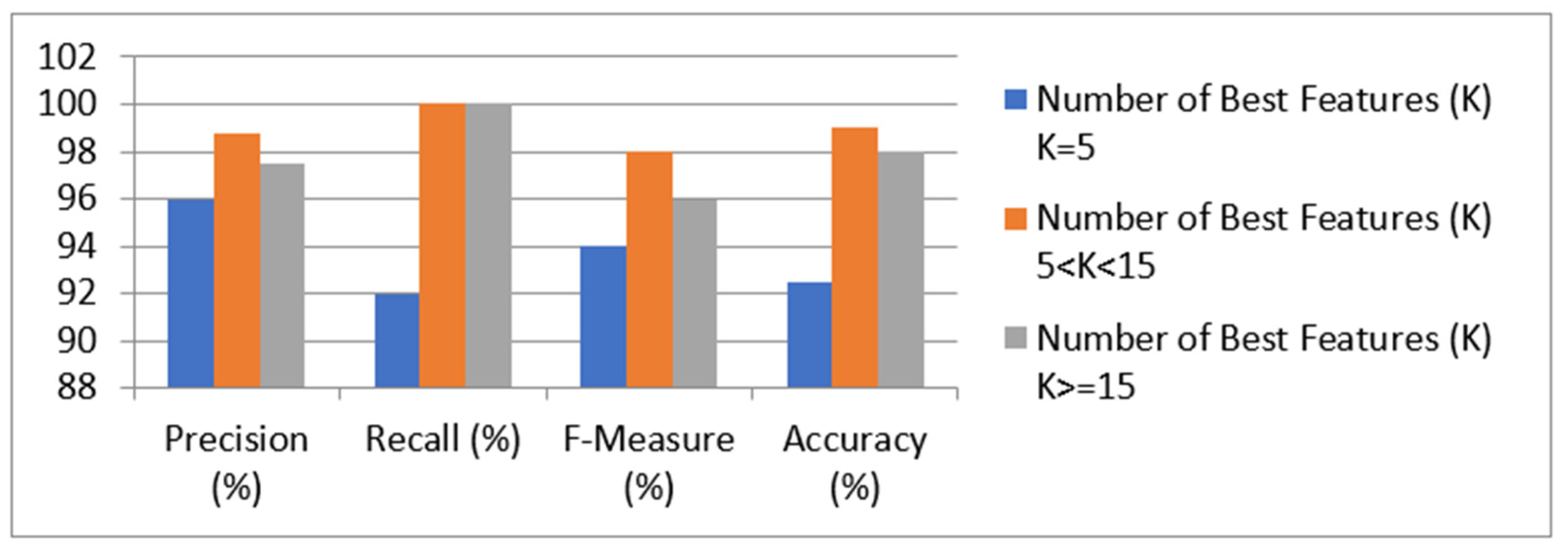
| Performance Measure | Number of Features (K) | Best K > = 15 |
|---|---|---|
| K = 5 5 < K < 15 | ||
| Precision (%) | 96 100 | 100 |
| Recall (%) | 92 98 | 96 |
| F-Measure (%) | 94 99 | 98 |
| Accuracy (%) | 92.5 98.75 | 97.5 |
| Method | Accuracy | Recall | Precision | F-Measure |
|---|---|---|---|---|
| Logistic regression [28] | 91.8 | 1 | 0.98 | 0.98 |
| KNN [29] | 92.7 | 0.88 | 0.98 | 0.92 |
| Naïve Bayes [30] | 95.21% | 0.92 | 1.00 | 0.94 |
| SVM [31] | 92.32 | 0.87 | 0.96 | 0.93 |
| Decision tree [32] | 93.45 | 0.95 | 1.00 | 0.96 |
| Proposed method [33] | 97.54 | 0.99 | 1.00 | 1.0 |
| Prediction Model | Accuracy (%) |
|---|---|
| Basic LR model | 91.25 |
| LR model + RFE feature selection | 97.5 |
| LR model + Chi-Square feature selection (K = 5) | 92.5 |
| LR model + Chi-Square feature selection (5 < K < 14) | 98.75 |
| LR model + Chi-Square feature selection (K > 14) | 97.5 |
Publisher’s Note: MDPI stays neutral with regard to jurisdictional claims in published maps and institutional affiliations. |
© 2022 by the authors. Licensee MDPI, Basel, Switzerland. This article is an open access article distributed under the terms and conditions of the Creative Commons Attribution (CC BY) license (https://creativecommons.org/licenses/by/4.0/).
Share and Cite
Poonia, R.C.; Gupta, M.K.; Abunadi, I.; Albraikan, A.A.; Al-Wesabi, F.N.; Hamza, M.A.; B, T. Intelligent Diagnostic Prediction and Classification Models for Detection of Kidney Disease. Healthcare 2022, 10, 371. https://doi.org/10.3390/healthcare10020371
Poonia RC, Gupta MK, Abunadi I, Albraikan AA, Al-Wesabi FN, Hamza MA, B T. Intelligent Diagnostic Prediction and Classification Models for Detection of Kidney Disease. Healthcare. 2022; 10(2):371. https://doi.org/10.3390/healthcare10020371
Chicago/Turabian StylePoonia, Ramesh Chandra, Mukesh Kumar Gupta, Ibrahim Abunadi, Amani Abdulrahman Albraikan, Fahd N. Al-Wesabi, Manar Ahmed Hamza, and Tulasi B. 2022. "Intelligent Diagnostic Prediction and Classification Models for Detection of Kidney Disease" Healthcare 10, no. 2: 371. https://doi.org/10.3390/healthcare10020371