Spatio-Temporal Traffic Flow Prediction in Madrid: An Application of Residual Convolutional Neural Networks

Abstract

Due to the need to predict traffic congestion during the morning or evening rush hours in large cities, a model that is capable of predicting traffic flow in the short term is needed. This model would enable transport authorities to better manage the situation during peak hours and would allow users to choose the best routes for reaching their destinations. The aim of this study was to perform a short-term prediction of traffic flow in Madrid, using different types of neural network architectures with a focus on convolutional residual neural networks, and it compared them with a classical time series analysis. The proposed convolutional residual neural network is superior in all of the metrics studied, and the predictions are adapted to various situations, such as holidays or possible sensor failures.

1. Introduction

Madrid is a smart city and is one of the five most populated cities in the European Union, with 3.1 million inhabitants and approximately 1.7 million vehicles circulating through its streets. A traffic forecasting system is essential for managing the growing volume of vehicles in these cities. In this respect, traffic flow prediction has received special attention in the last two decades [1]. Using spatio-temporal data [2] obtained from a range of sensors, a variety of real-world problems can be solved, such as the demand for taxis [3,4,5], urban traffic control and congestion avoidance [6,7], abnormal event detection [8,9], and travel time estimation or route planning [10,11,12], amongst others.

1.1. Related Work

Traffic flow prediction can be considered as using past and current flow data to predict traffic in the near future [13]. Many studies have proposed various traffic flow prediction methodologies [14] for both short- (seconds to 1 h) and long-term (more than 1 h) estimation. Short-term traffic flow prediction has recently received increasing scientific and research interest, which is mainly due to several advances in the application of artificial intelligence in this field [15]. In addition, the use of deep neural networks for regression is a current research topic [16,17].

The classical methods of time-series analysis that have been applied to short-term traffic flow forecasting include autoregressive integrated moving average (ARIMA) models or hybrid models with ARIMAS [18,19,20]. Several types of neural networks for time series have shown superior performance to that of these linear models. Examples of these include recurrent neural networks (RNNs), which integrate feedback loops that allow information to persist for a few epochs through layer connections by embedding their results in the input data [21,22]. The connections between nodes form a directed graph along a time sequence. This creates an internal state that allows the memorization of previous data. However, the training of RNNs is costly in terms of time and memory use. When longer time sequences are analyzed, the vanishing gradient problem may appear. Another class of networks that are capable of monitoring previous data is the class of long short-term memory (LSTM) networks [23]. This type of network solves the vanishing gradient problem. LSTM networks work with long delays and are superior to other methods in many applications, such as language learning [24] and connected handwriting recognition [25], amongst others.

The first examples of these advances can be found in deep stacked autoencoder networks [26,27] and LSTM neural networks [28,29,30]. Other deep learning architectures have been adopted in this research area and have produced many encouraging results. Later, works using deep learning focused on traffic flow prediction using stacked autoencoders [21] and deep belief networks [31]. However, these models were too shallow to adapt to nonlinear structures and to learn multimodal patterns in traffic data [2]. More recent works have used residual convolutional neural network (ResNet)-type deep neural networks [32] and LSTM networks for traffic flow prediction [1,33]. In previous studies [34,35], a ResNet was used for traffic flow prediction with multitask learning and flow-map super-resolution, and it showed high efficiency and effectiveness in prediction. There are even studies that combine RNNs and CNNs [2,5], although this is usually performed by sliding windows over a map.

Several studies based on spatio-temporal data have recently been conducted with the aim of predicting, for example, the next destination [36,37,38]. These studies mostly focused on analyzing patterns of individuals rather than viewing the problem as a global whole.

1.2. Overview

The spatial relationships between sensors could be important because the traffic flow in one location can be affected by abnormal events in locations nearby, such as traffic accidents, road closures, and certain types of events, such as demonstrations or sporting events, which could have an important impact on the traffic situation [39]. Convolutional neural networks (CNNs) can be a possible solution to this problem because they contemplate the spatio-temporal structure of the set of sensors. As such, the aim of this study was to perform a short-term prediction of traffic flow in Madrid using different types of neural network architectures. Unlike most of the works presented in the recent literature, in this paper, we would like to use an approach that is not based on sliding windows, but receives the full map of the city to facilitate the consideration of long-distance relationships. In addition, ResNet is a more powerful deep architecture that is based on CNN and takes advantage of the similarity between the input and the output required in the network. For this reason, we adopted a ResNet for this problem and compared it with methods based on a classic time-series analysis.

2. Materials and Methods

In Section 2.1, we will explain our dataset and the division in it; one part is used to create the model and the other is used to test it. In Section 2.2, we present the non-visual models designed to solve the regression problem. These models are the ones that have classically been used for this type of problem [40]. In this subsection, we introduce the elements needed to address this problem using ARIMA models. Finally, in Section 2.3, we present our proposed visual model.

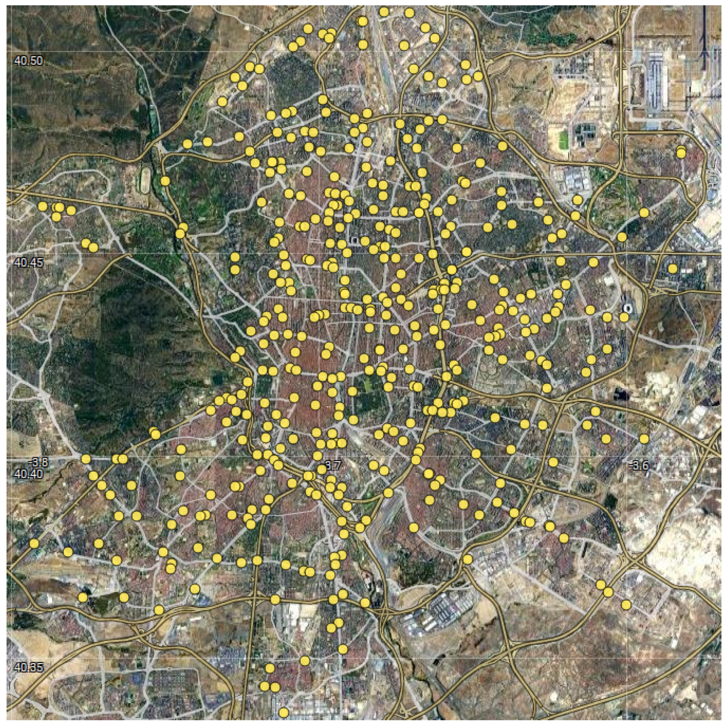
2.1. Study Design and Data Source

For the different experiments performed in this work, we use a dataset obtained from the open data page of the Madrid City Council (https://datos.madrid.es/portal/site/egob/menuitem.c05c1f754a33a9fbe4b2e4b284f1a5a0/?vgnextoid=33cb30c367e78410VgnVCM1000000b205a0aRCRDvgnextchannel=374512b9ace9f310VgnVCM100000171f5a0aRCRDvgnextfmt=default (accessed on 10 May 2021). This portal provides a detailed history of the traffic flow data from all fifteen since 2013. The data were obtained from 4200 sensors distributed along Madrid’s roads (Figure 1). All of the sensors were static in fixed points on roads of the city. At the time of this study, the following information was available: date, hour, sensor identifier, type of sensor (urban or bypass highway), traffic flow intensity of the sensors in 15 min periods (vehicles/hour), occupancy of the road (measuring point’s occupancy time in the 15 min periods; in percentage), load (vehicle loading in the 15 min period (considering the intensity, occupancy, and capacity of the road, from 0 to 100)), average speed of vehicles in a 15 min period (km/h; only for sensors located along bypass highways), and indications of there being at least one incorrect or substituted sample in the 15 min period.

Because the website did not have an application programming interface for downloading these data, the data were obtained by webscraping to collect all traffic information from 1 January 2016 to 31 December 2019. These data were divided into two disjoint sets: a training dataset and a testing dataset. The training dataset was composed of the traffic information from 1 January 2016 to 31 December 2018. The testing dataset was composed of the traffic information from 1 January 2019 to 31 December 2019. Note, the more recent data were used for testing, in order to ensure the generalization capability of the models. The traffic flow intensity data (number of vehicles/hour) comprised our target variable, and the average of the data collected every fifteen minutes was considered a grouping, i.e., data at the hourly level were constructed. In addition, erroneous data (from the indicator or when an observation was not provided) were considered as missing data.

Only measurement points that provided data in the four years of study (2016–2019) were considered, as some measurement points were temporary and were not collected in all years. We used 2016–2018 for training and 2019 for testing.

To train the models, missing data from the training series were filled in by using the closest previous data by day of the week and time from the rest of the series. For all of the treatments, a total of 3400 series were considered. All of the information regarding the sensors and their spatial locations can be downloaded from the following link (https://datos.madrid.es/portal/site/egob/menuitem.c05c1f754a33a9fbe4b2e4b284f1a5a0/?vgnextoid=ee941ce6ba6d3410VgnVCM1000000b205a0aRCRD&vgnextchannel=374512b9ace9f310VgnVCM100000171f5a0aRCRD (accessed on 10 May 2021).

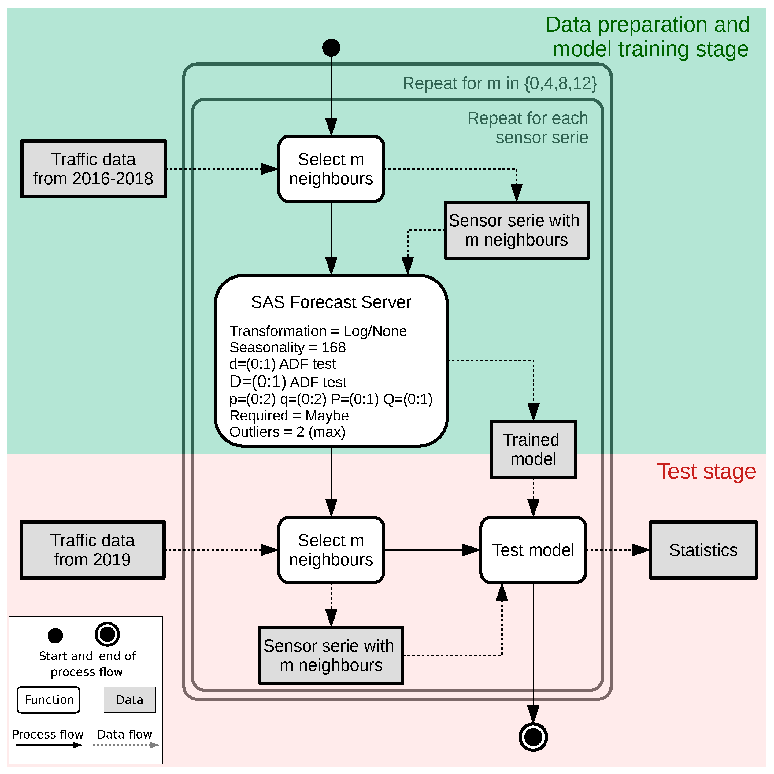
2.2. ARIMA Models

ARIMA models, which are generalizations of the autoregressive moving average (ARMA) model, are standard in the field of time-series forecasting. As Box and Jenkins stated in their methodology [41], to fit models of this type, it is first necessary to guarantee the stationarity—in a weak sense—of the time series to be modeled.

In our study, we considered two types of seasonalities: one depends on the time of day (s = 24), and the other depends on the day of the week (s = 24 × 7 = 168). However, forecast server only refers to one of the two, a limitation that we also found in the auto.arima function. To overcome this problem, we decided to specify the value corresponding to the strongest seasonality for s and to reflect the other periodicities by including regressors.

To decide which of the two seasonalities is stronger, as ARIMA models are linear in nature, the linear correlations between the data of the series in question and the same data lagging by 24 and 168 time units were calculated for each series:

$$\left\{\begin{array}{c}cor{r}_{24}^{i{d}_{serie}}=corr\left(i{d}_{seriet-24}\right)\hfill \\ \mathrm{and}\hfill \\ cor{r}_{168}^{i{d}_{serie}}=corr\left(i{d}_{seriet-168}\right)\hfill \end{array}\right.\forall i{d}_{serie}\in \left(1,2,\dots ,3400\right)$$

With the 3400 pairs of values $\left(cor{r}_{24}^{i{d}_{serie{s}_{i}d}},cor{r}_{168}^{i{d}_{series}}\right)$, a nonparametric Kruskal–Wallis test was performed to determine any significant differences between these correlations, which showed that they were higher for $cor{r}_{168}^{i{d}_{series}}$.

For this reason, models of the type $SARIMA(p,d,q)x{(P,D,Q)}_{168}$ were fitted (Figure 2), and the seasonality of order 24 was reflected through regressors. Two alternatives were tested: to generate dummy variables associated with each of the 24 h of the day or to consider a single regressor referring to the value of the series in question 24 time periods ago—an effect that, in the end, reflected at least an AR(24) structure. The computational cost involved in reflecting the high number of regressors of the former led us to opt for the latter, after having verified that the results obtained for a sample of the series with respect to the magnitude of the prediction errors with one another, were not significantly different from a statistical point of view.

Regarding the value of the possible orders proposed for the model $SARIMA(p,d,q)\times {(P,D,Q)}_{168}$, the value of 2 was specified for the orders p and q, as it was not realistic for the traffic of one hour to be conditioned by the traffic of more than two hours before. A similar reasoning led us to limit the value of the parameters P and Q to 1. The number of differences was set to 1, as the maximum value for d and D (Figure 2), because it was not realistic to consider higher orders. Thus, a value of $d=2$ would be justified for a series that shows quadratic trends, a behavior that was not observed in any of the modeled series. Thus, the contrasted models responded in an extreme case to an expression of the type:

$$X_t={\beta }_0+\frac{\left(1-{\theta }_{1}B-{\theta }_2{B}^2\right)\left(1-{\Theta }_1{B}^{168}\right)}{\left(1-{\varphi }_{1}B-{\varphi }_2{B}^2\right)\left(1-{\Phi }_1{B}^{168}\right)\left(1-B\right)\left(1-B^{168}\right)}{ϵ}_t+w{X}_{t-24}$$

(1)

where $X_t$ can be each of the original series or their respective logarithm transformations.

Regressors associated with the traffic of neighboring zones in the hour immediately prior to that for which the prediction is proposed were considered (Figure 2), so that the final equation of the model for predicting the traffic flow associated with a zone j responds to a structure of the type:

$$\begin{array}{cc}\hfill X_{t-1}^j=& {\beta }_0+\frac{\left(1-{\theta }_{1}B-{\theta }_2{B}^2\right)\left(1-{\Theta }_1{B}^{168}\right)}{\left(1-{\varphi }_{1}B-{\varphi }_2{B}^2\right)\left(1-{\Phi }_1{B}^{168}\right)\left(1-B\right)\left(1-B^{168}\right)}{ϵ}_t+\hfill \\ \hfill & +w{X}_{t-24}+\sum _{i\in B(j,m),i\ne j}{\nu }_t{X}_{t-1}^i\hfill \end{array}$$

(2)

where $B(j,m)$ is a ball that includes the m zones closest to j, where m = 4, 8, and 12. In Equation (2), only input variables whose parameters are statistically significant (required = maybe, Figure 2) are considered. Finally, ARIMA models are sensitive to the existence of outliers. The Forecast Server tool has a procedure for automatically identifying outliers. Based on these data, the tool generates intervention variables to take their effect into account so that they do not affect the quality of the predictions that it generates. The process of identifying outliers is computationally expensive; therefore, the maximum number of variables of this type to be considered in each model was reduced to 2 (Figure 2).

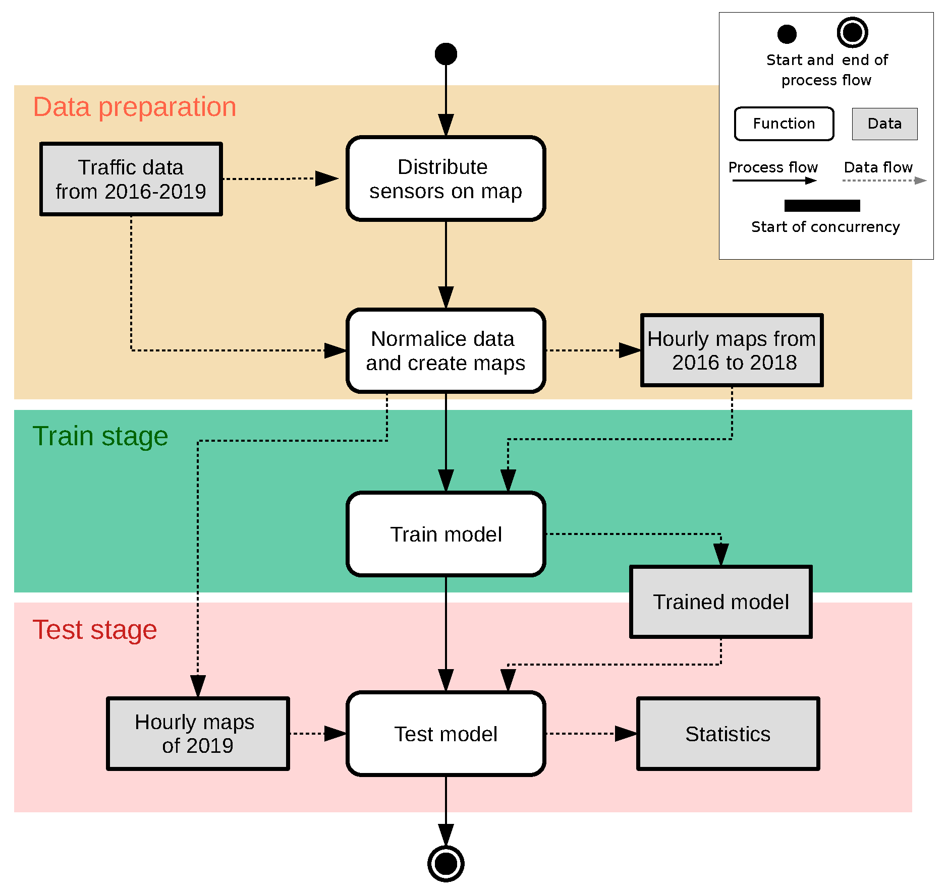
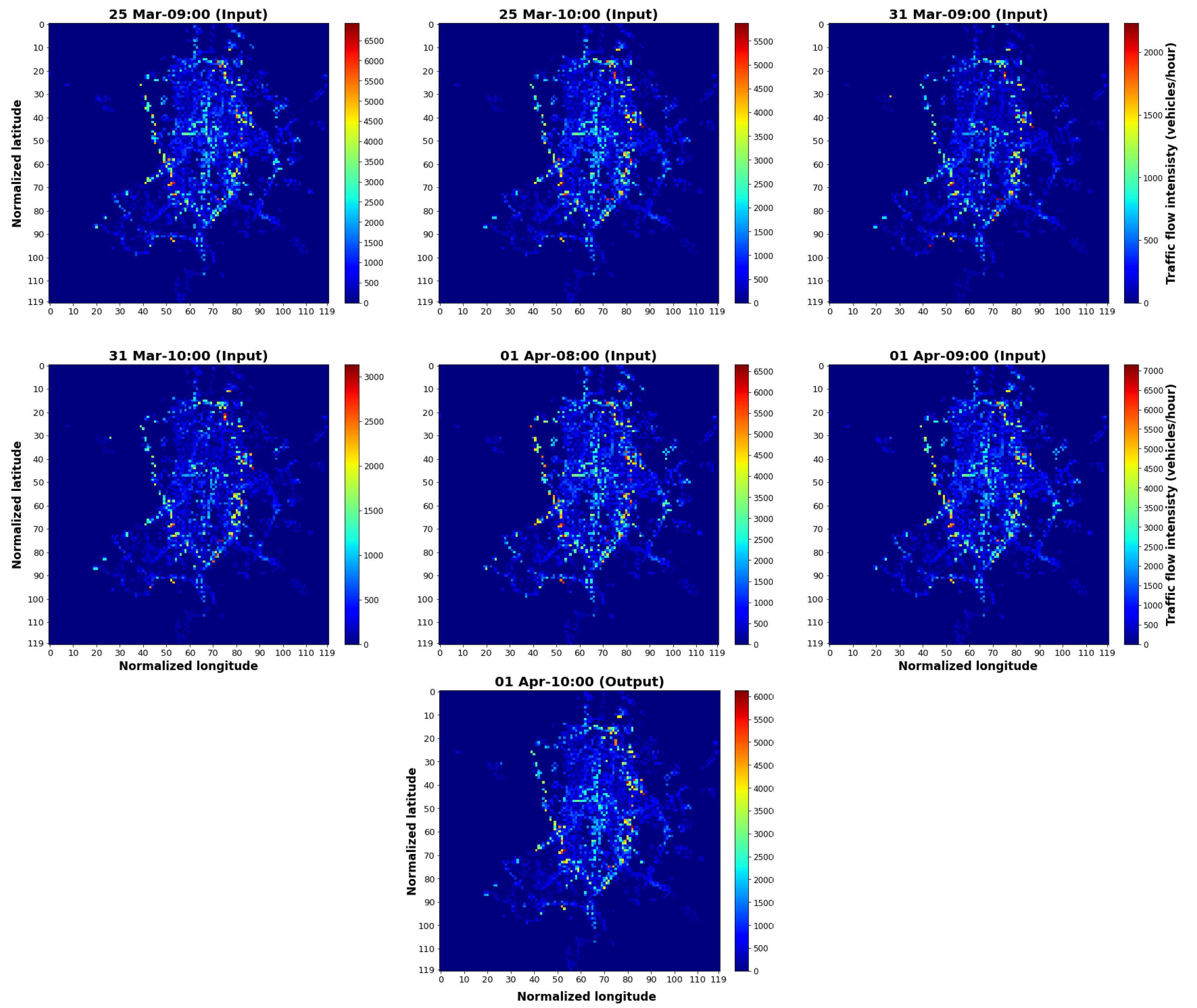
2.3. Visual Model

In this subsection, we present some necessary data preparations for the visual models. Later, we present a very basic visual model based on a CNN. Finally, we present the main contributions of this work: a modification of a ResNet for solving the regression problem applied to traffic flow prediction.

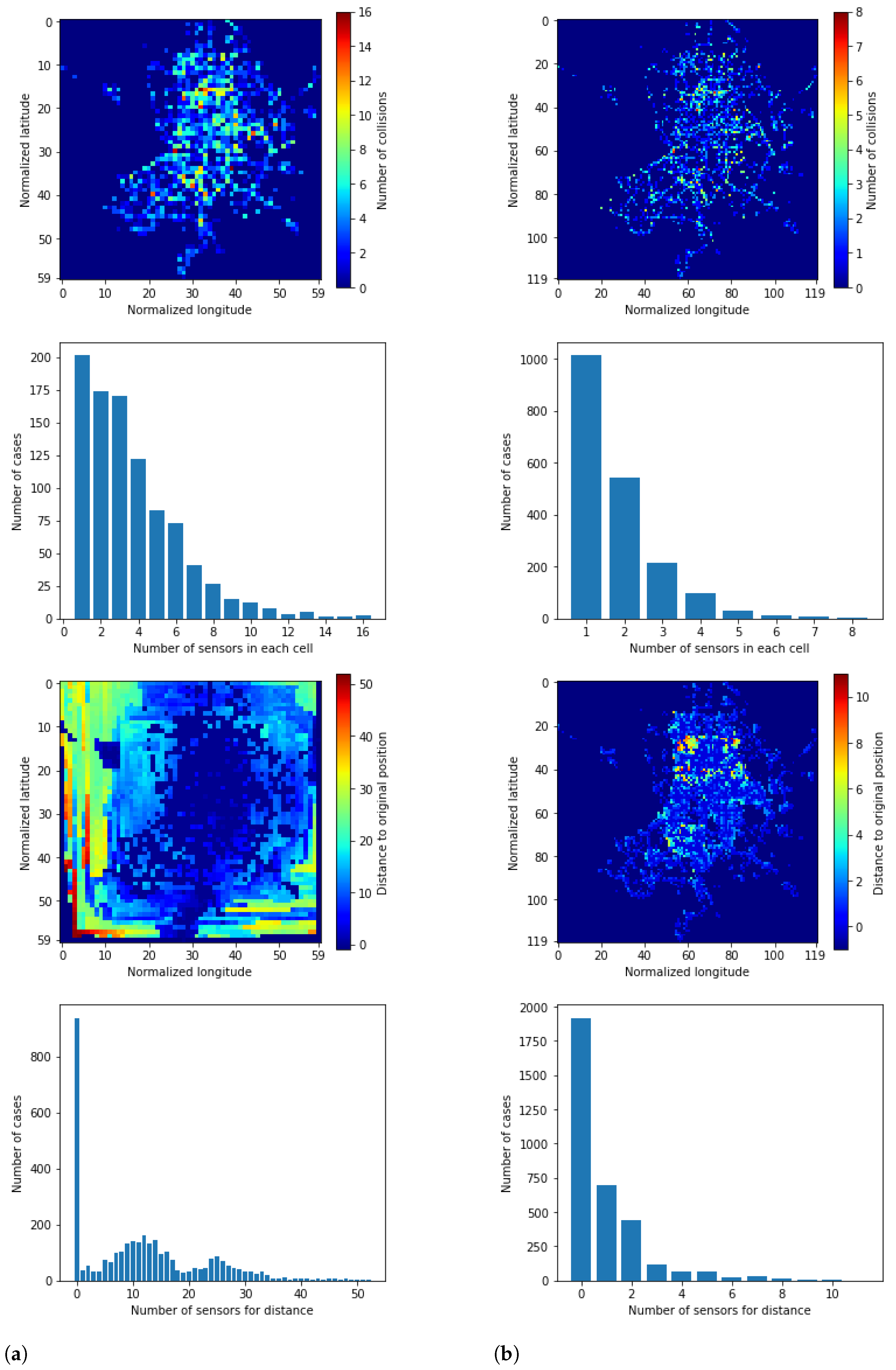
2.3.1. Data Preparation

The input for the visual model was a sequence of maps related to the traffic flow values recorded by the sensors at different time instants. The instants chosen were the same as those in the ARIMA model. So, to predict the map corresponding to the instant t, maps for capturing the trend of the previous hour $(m_{t-1},m_{t-2})$, of the same hour on the previous day $(m_{t-24},m_{t-25})$, and of the same hour in the previous week $(m_{t-24·7},m_{t-24·7-1})$, were used as input. As output, this visual model provided a map corresponding to the traffic flow prediction for a later time $m_t$.

Each map m is presented as an $N\times N$ matrix of real numbers. Each point $p(i,j)$ of this matrix contains the traffic flow value at latitude i and longitude j of the map. A square matrix was chosen because the map of Madrid is approximately square (Figure 1). The points on the map that correspond to the geolocation of a sensor take the value of the sensor at that instant. The points of the matrix that do not correspond to positions with sensors are kept at zero.

The matrix dimensions must be chosen by considering two aspects. First, if N is small, the computation time and memory usage of the networks will be lower, but there may be overlap between the positions of sensors that are close to each other. This is due to sensors in the center of the city being very close, but there are sensors in the outskirts of the city that are far away from each other. If N is large, the overlap is reduced, but it penalizes the training process in several ways: First, the amount of memory needed to load the matrix is very high. Second, the neural network has many weights to store and adjust. Third, this large matrix is very sparse because the number of sensors is fixed to 3400 and the matrix grows quadratically.

With 3400 sensors, the minimum value of N is approximately 60. However, if we fix $N=60$, many sensors overlap (see the first and second rows of Figure 3a). We also tried configurations of $N=120$, but, again, several sensors overlapped (see the first and second rows of Figure 3b).

To solve this issue, we built an algorithm that assigns each sensor to the corresponding position in an $N\times N$ matrix in the case of an overlapping search for the nearest empty position (Algorithm 1).

Using the assignment algorithm, we could situate the 3400 sensors in a minimal matrix with $N=60$, but sometimes, the position of a sensor was assigned to a cell that is far from its original position (see the third and fourth rows of Figure 3a). This penalizes the local behavior being searched for with any visual approach. However, when $N=120$, these distances are greatly reduced (see the third and fourth rows of Figure 3b).

Algorithm 1: Algorithm that searches for an empty cell near a given position.

Figure 4 describes the activities involved in the training and testing stages of the visual model. The data preparation stage is executed only at the beginning of the process, and it consists of two activities: the execution of the explained algorithm to distribute the sensors in the matrix and a normalization of the data to be in the [0,1] range, which is performed by dividing the data by the maximum. This normalization is common in network training because the highest resolution is around zero in floating-point systems. Then, all of the maps are created before the training stage. Thus, maps of 24 h × 365 days × 3 years are loaded into the memory. An example of the input pattern and expected pattern generated by our model is shown in Figure 5; these patterns show a strong spatio-temporal relationship between the input and the output.

Note that our visual approximation only needs to train one model for all of the sensors, in contrast to ARIMA’s training process, in which it is necessary to train a model for each sensor. In addition, note that all of the sensors are processed in parallel by using matrices, without the need for loops.

2.3.2. Preliminary Visual Model: Regression CNN

To take advantage of the spatial information related to the positions of the measurement stations, first, we propose the use of a deep model based on CNNs. This is perhaps the simplest model based on deep learning, and it was inspired by the work of LeCun et al. in 1998 [42].

This resulted in the following equation, which was implemented in the network shown in Figure 6.

$$m_t\approx CNN(m_{t-1},m_{t-2},m_{t-24},m_{t-25},m_{t-24\times 7},m_{t-24\times 7-1})$$

(3)

If the network has three layers of a CNN with a $5\times 5$ kernel size, each sensor of the matrix could affect sensors that are in a $13\times 13$ neighborhood (Figure 7). When $N=60$, there are very geographically near sensors that are positioned outside of this $13\times 13$ neighborhood (see the fourth row of Figure 3a). However, when $N=120$, as can be seen in the fourth row in Figure 3b, all sensors are in a neighborhood of $10\times 10$ with respect to their original positions. Thus, we chose $N=120$ for the input and output layers of the models, as well as at least three levels of convolutional layers.

The training stage uses a mean square error loss function with the Adam algorithm to fit the weights of the neural network. The training data were divided into training (from 2106 and 2017) and validation (from 2018) subsets. The network was trained until no improvement was detected in the validation data in the last 100 epochs. In each epoch, all of the samples were presented to the network in batches of 32 samples.

Unlike the LeCun model, as the output had the same size as the input, a maxpooling layer was not needed. In addition, the final dense layer was substituted by a $7\times 7$ convolutional ReLu layer. Finally, we found that only dropout regularization layers could be used, due to the effects of normalization introduced by the Euclidean distance (L2 norm) or batch-normalization regularization on the linear output.

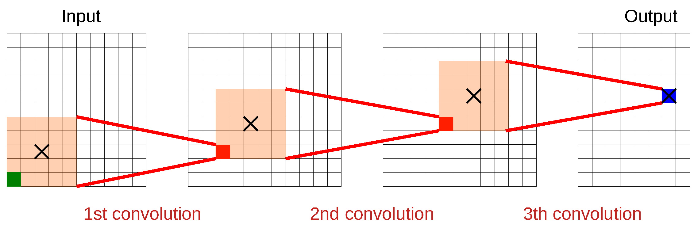
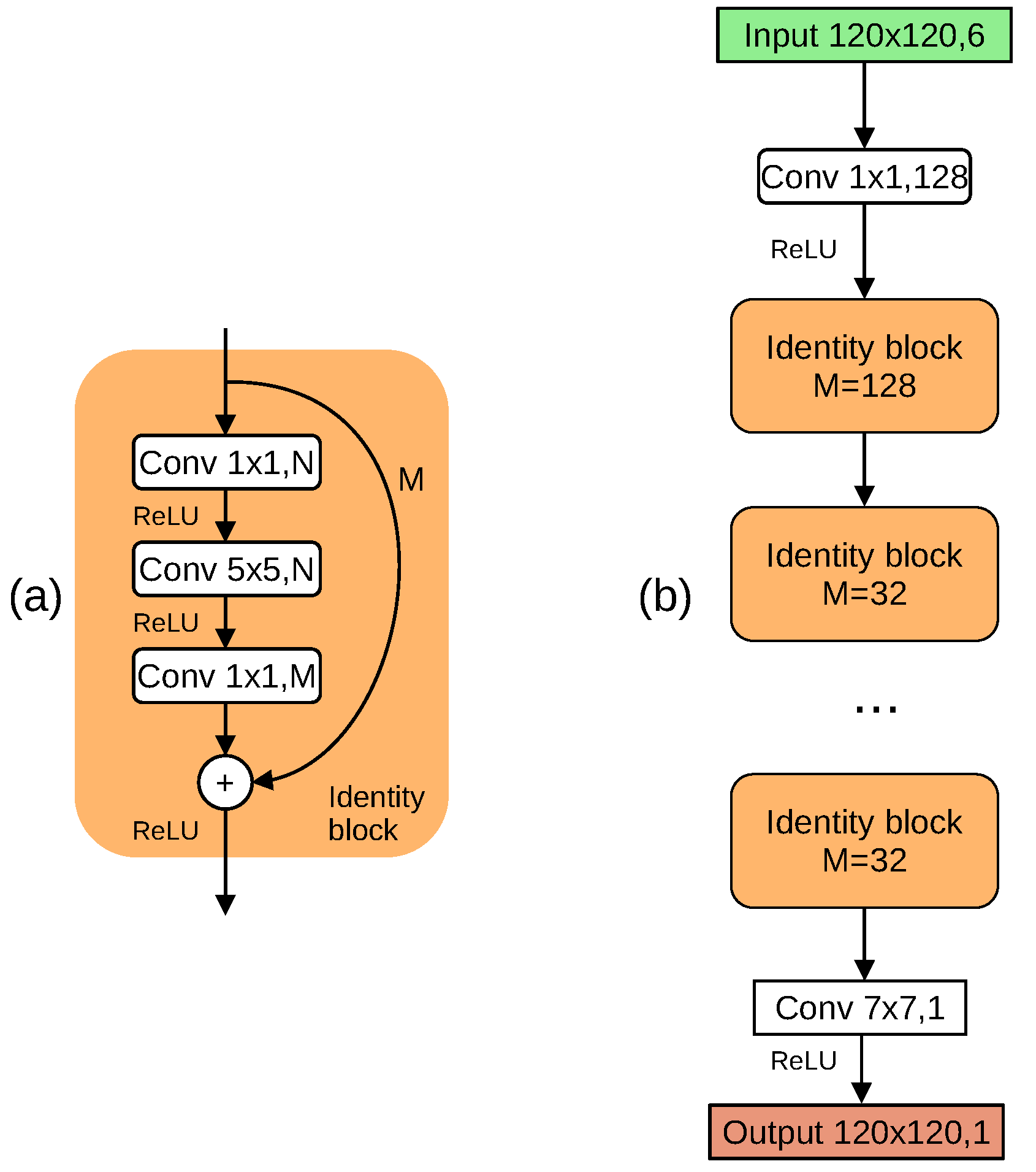
2.3.3. Regression ResNet Model

As the prediction for the instant t can be seen as the map corresponding to $t-1$ plus a residual, we thought that the use of residual networks could improve the CNN results. Formally, this can be expressed as:

$$m_t\approx m_{t-1}+r$$

(4)

Note that Equation (4) is in line with Equation (5) from He et al. [32] for residual networks.

$$y=F(x,\left\{W_i\right\})+x$$

(5)

where x is $m_{t-1}$, F is the function corresponding to the neural network, $W_i$ are the weights of this net, and y is the desired prediction $m_t$.

Just as CNNs are based on the concatenation of convolutional layers, ResNet networks are based on the concatenation of linear blocks. As linear blocks, we used the deeper bottleneck architecture proposed by [32] (see Figure 8a). In their proposal, each linear block contained three convolutional layers with a ReLU activation function.

The 1 × 1 layers reduce and increase the previous dimensions, while the 5 × 5 layer creates a bottleneck with smaller input/output dimensions. Finally, there is a shortcut that adds the input directly to the output of the linear block. Using this idea and adding the maps corresponding to previous time instants of Equation (3) to the input, we obtain Equation (6), which is implemented in the architecture in Figure 8b.

$$m_t\approx ResNet(m_{t-1},m_{t-2},m_{t-24},m_{t-25},m_{t-24\times 7},m_{t-24\times 7-1})$$

(6)

After some experiments, we set the hyperparameters in a slightly different way compared to the proposal in [32]. In particular, we always set N to 32 and M to 128. However, the more important change was the substitution of the first $7\times 7$ convolutional layer of the original ResNet for a 1 × 1 convolutional layer. This is because we needed the maps of previous hours to be unmodified in each layer.

As in the CNN case, maxpooling layers were not needed, and batch normalization produced worse results. Finally, the last dense layer was substituted by a $7\times 7$ convolutional layer with ReLu activation.

2.4. Performance Indexes

To evaluate the effectiveness of the proposed model, we used three performance indexes: mean absolute error (MAE), mean absolute percentage error (MAPE), and symmetrical mean absolute percentage error (SMAPE). They are defined as:

$$\begin{array}{cc}\hfill MAE& =\frac{1}{n}\sum _{t=1}^n|y_t-\widehat{y_t}|\hfill \\ \hfill MAPE& =\frac{100\%}{n}\sum _{t=1}^n\frac{|y_t-\widehat{y_t}|}{y_t}\hfill \\ \hfill SMAPE& =\frac{100\%}{n}\sum _{t=1}^n\frac{|y_t-\widehat{y_t}|}{|y_t+\widehat{y_t}|}\hfill \end{array}$$

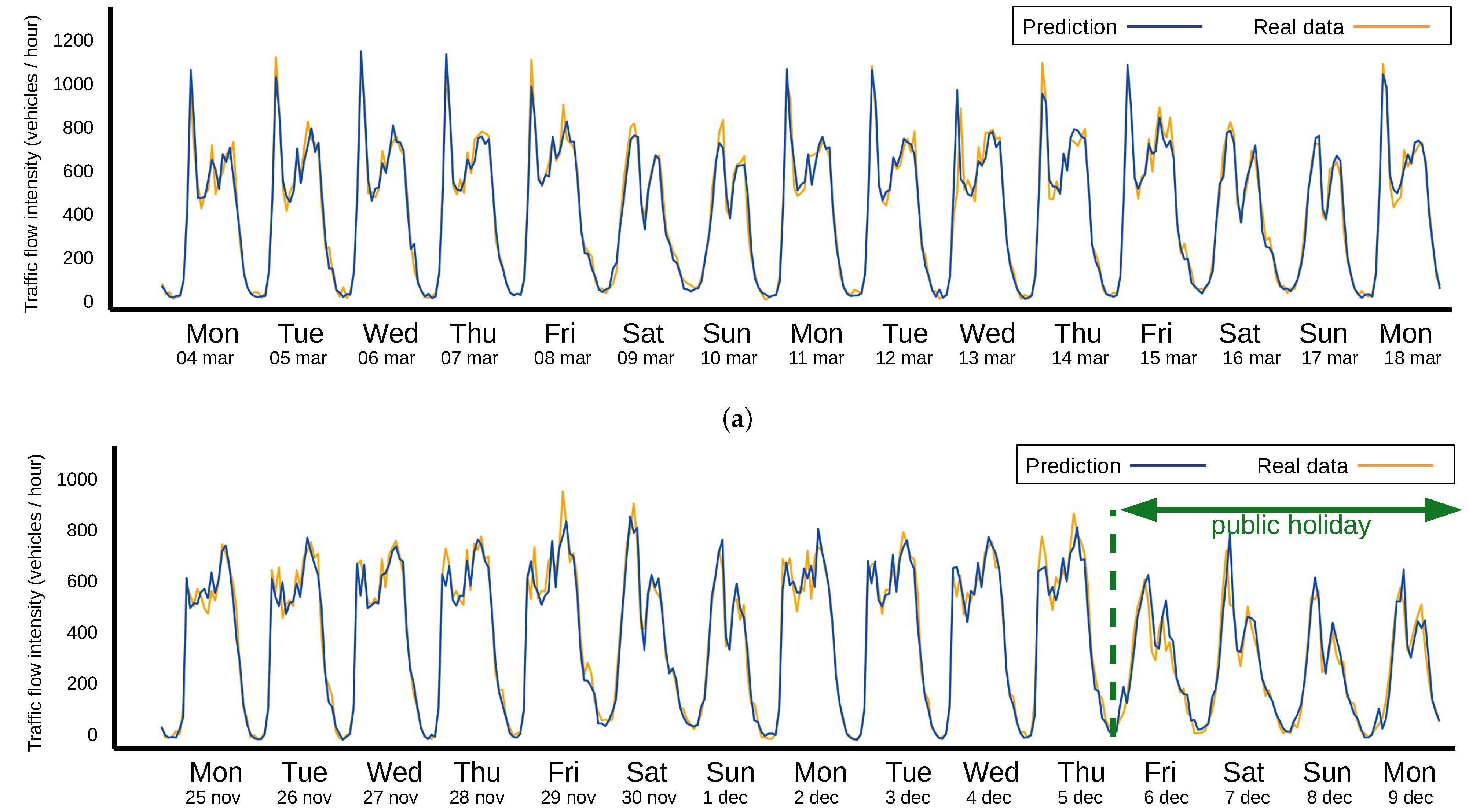
3. Results

In this section, we provide the results obtained with all of the proposed models (regression CNN, regression ResNet, and ARIMA models) on the test dataset described in Section 2.1.

Table 1. Results obtained on the 2019 testing dataset with all of the proposed models. MAE, mean absolute error; MAPE, mean absolute percentage error; SMAPE, symmetrical mean absolute percentage error.

Model Details		Results
Model	Parameters	MAE	MAPE	SMAPE
ARIMA	27,200	40.85	20.00%	9.50%
ARIMA ($m=4R$)	40,800	40.45	19.81%	9.35%
ARIMA ($m=8R$)	54,400	40.22	19.75%	9.33%
ARIMA ($m=12R$)	69,000	40.11	19.78%	9.35%
CNN ($c=3$)	7169	51.65	22.79%	11.82%
CNN ($c=4$)	154,753	51.52	22.62%	11.56%
CNN ($c=5$)	302,337	50.98	22.45%	11.21%
ResNet ($i=2$)	109,601	38.93	18.75%	9.35%
ResNet ($i=3$)	262,049	37.92	18.22%	8.29%
ResNet ($i=4$)	482,465	39.65	19.08%	9.16%

presents the performance indexes of the models proposed in Section 2 on the testing dataset corresponding to 2019, with all of the models trained with data from 2016 to 2018. The ARIMA model corresponding to Equation (1) (which only considers the historic traffic flow of the involved sensor) obtained an MAE of 40.85. The ARIMA model according to Equation (2) (which considers regressors associated with the traffic flow measured in the m-closest positions) obtained slightly better results. For m = 4, 8, and 12, the model obtained an MAE of 40.45, 40.22, and 40.11, respectively. A similar pattern was observed for MAPE and SMAPE, except when $m=12$, for which MAPE and SMAPE did not improve.

The CNN and ResNet models were trained over 500 epochs. In each epoch, all of the training patterns (hourly from 2016 to 2018) were presented to the network. The model that obtained the best validation result was selected for testing. The validation set was composed of non-overlapping 20% portions of the training set.

Table 1 shows that the CNN models obtained competitive results. The CNN with three convolutional layers ($c=3$) obtained an MAE of 51.65. CNNs with more convolutional layers obtained similar results. Note that the CNNs’ results were no better than those obtained by the ARIMA models.

Finally, the ResNet models obtained better results compared with all of the previous approaches. Thus, the ResNet with two identity blocks ($i=2$) obtained an MAE of $38.93$, and the ResNet with three identity blocks ($i=3$) obtained the best results with an MAE of $37.92$. Again, a similar pattern was observed for MAPE and SMAPE. This configuration improved the results of the best ARIMA model in all of the measures: 37.92 vs. 40.11 for MAE, 18.22% vs. 19.75% for MAPE, and 8.29% vs. 9.33% for SMAPE.

The inclusion of four identity blocks in the ResNet model ($i=4$) did not improve the results obtained when $i=3$ (Table 1) due to the training being stopped after 500 epochs. In our experiments, we trained this configuration with more epochs, and then we achieved the results for $i=3$. However, the results were not significantly better; we believe that more complex networks (with $i>3$) would not improve the results obtained with the $i=3$ configuration.

In the analysis of the results, the inclusion of explanatory variables in the ARIMA models did not significantly improve the quality of the predictions. Similarly, even the best ARIMA prediction was far from having the predictive ability obtained with the ResNet in the considered measures.

Figure 9a shows the predictions vs. the real data in a succession of 15 common days. ResNet adjusted to the real data in a reliable manner and was capable of capturing the different peaks of traffic flow in a common day, such as the early hours of the morning and the afternoon, which correspond to work commuting times. Notably, ResNet could adapt its predictions to rare events. Figure 9b shows the predictions for a public holiday in Madrid (December 6). On this day, the flow traffic was significantly lower than on the same day of the previous week. This showed the adaptability of ResNet to prediction in short time periods. Our ResNet was able to adapt its predictions to unexpected events, as shown in Figure 9c, which depicts the predictions for what appears to be a possible sensor failure.

4. Discussion

One of the limitations of ARIMA-based time-series models is that they do not consider the spatial structure of the set of sensors, which can only be achieved by adding explanatory variables to each fitted model. Fit-vector ARMA models can be used, but the computational cost is very high. In relation to the latter, our model proposes a modification that is easy to implement based on ResNet-type networks. We considered traffic flow as having an important spatial component, because what happens in one area at a given time can influence what happens in another part of the city in the following hour. This component allowed us to present the measurements of a specific instant to create an image of a map of the city at a moment in time. The possibility of training on a city as a whole allows the model to learn specific behaviors relative to one city, which cannot be captured by more local models.

Perhaps, it would be interesting to maintain the dense layer that is usually positioned in the last layers of several deep architectures. However, due to the absence of maxpooling layers, this dense layer would add several millions of parameters to our model ($120\times 120\times 120\times 120$), and our model would not be trainable in a reasonable amount of time. The use of convolutional layers in the linear block is also an advantage over the proposal of [16], who used dense layers, and this increases the number of parameters again. It can be noted that our changes to the original ResNet proposal are in concordance with the results of S. Lathuiliere [17], except that we obtained better results when the input was similar to the original map ($N=120$).

We constructed a model that is able to accurately predict the traffic flow and to adapt to unforeseen patterns such as certain sporting events or the stopping of measurement at the sensor; it can be extrapolated to other real-life examples that take space–time measurements as input data, such as weather forecasting or environmental conditions. We only compared our model against a single model based on time series, but we did not compare it with LSTM or hybrid networks. In the future, our model can be compared using stochastic partial differential equations (SPDEs) [43], as the placed sensors can be considered as a Gaussian field that is affected by a measurement error and state process and is spatially correlated. This can be achieved by using the integrated nested Laplace approximation [44].

From our point of view, our model provides two contributions to spatio-temporal problems: We showed that deep learning provides an important improvement over linear models, such as ARIMA or SARIMA, and neural networks were shown to be a very dynamic research area where there is still much room for improvement compared with the more classical methods.

We think that other recent architectures, such as “inception” or “you only look once” (YOLO), are very powerful for problems in which there are changes in resolution between the input patterns. However, this is not the case in this problem. Thus, we think that these approaches will not improve our results. However, the use of encoder–decoders or the use of attention mechanisms could improve our results.

5. Conclusions

This paper presented an adaptation of a ResNet for the spatio-temporal estimation of short-term traffic flow in a large city: Madrid, Spain. The proposed network proved to be superior to SARIMA models in terms of prediction accuracy. The proposed model is easily applicable to traffic flow prediction and is extensible to other real-life situations involving spatio-temporal structures, such as pollution or temperature prediction.

In future work, we will study the possibility of adding an encoder–decoder stage to our ResNet model in order to consider data from very distant sensors. Another future objective is to test our model in other cities and in other situations that involve spatio-temporal structures.

References

- Wang, W.; Zhang, H.; Li, T.; Guo, J.; Huang, W.; Wei, Y.; Cao, J. An interpretable model for short term traffic flow prediction. Math. Comput. Simul. 2020, 171, 264–278. [Google Scholar] [CrossRef]
- Zhou, F.; Li, L.; Zhang, K.; Trajcevski, G. Urban flow prediction with spatial–temporal neural ODEs. Transp. Res. Part Emerg. Technol. 2021, 124, 102912. [Google Scholar] [CrossRef]
- Liu, T.; Wu, W.; Zhu, Y.; Tong, W. Predicting taxi demands via an attention-based convolutional recurrent neural network. Knowl. Based Syst. 2020, 206, 106294. [Google Scholar] [CrossRef]
- Zhang, C.; Zhu, F.; Wang, X.; Sun, L.; Tang, H.; Lv, Y. Taxi Demand Prediction Using Parallel Multi-Task Learning Model. IEEE Trans. Intell. Transp. Syst. 2020, 1–10. [Google Scholar] [CrossRef]
- Zhang, D.; Xiao, F.; Shen, M.; Zhong, S. DNEAT: A novel dynamic node-edge attention network for origin-destination demand prediction. Transp. Res. Part Emerg. Technol. 2021, 122, 102851. [Google Scholar] [CrossRef]
- Qi, L.; Zhou, M.; Luan, W. A Two-level Traffic Light Control Strategy for Preventing Incident-Based Urban Traffic Congestion. IEEE Trans. Intell. Transp. Syst. 2018, 19, 13–24. [Google Scholar] [CrossRef]
- Afrin, T.; Yodo, N. A Probabilistic Estimation of Traffic Congestion Using Bayesian Network. Measurement 2021, 109051. [Google Scholar] [CrossRef]
- Dai, G.; Hu, X.; Ge, Y.; Ning, Z.; Liu, Y. Attention based simplified deep residual network for citywide crowd flows prediction. Front. Comput. Sci. 2021, 15, 152317. [Google Scholar] [CrossRef]
- Huang, C.; Zhang, C.; Zhao, J.; Wu, X.; Chawla, N.; Yin, D. MiST: A Multiview and Multimodal Spatial-Temporal Learning Framework for Citywide Abnormal Event Forecasting. In Proceedings of the International World Wide Web Conference, San Francisco, CA, USA, 13 May 2019; pp. 717–728. [Google Scholar]
- Ma, J.; Chan, J.; Ristanoski, G.; Rajasegarar, S.; Leckie, C. Bus travel time prediction with real-time traffic information. Transp. Res. Part Emerg. Technol. 2019, 105, 536–549. [Google Scholar] [CrossRef]
- Xu, S.; Zhang, R.; Cheng, W.; Xu, J. MTLM: A multi-task learning model for travel time estimation. GeoInformatica 2020. [Google Scholar] [CrossRef]
- Abdollahi, M.; Khaleghi, T.; Yang, K. An integrated feature learning approach using deep learning for travel time prediction. Expert Syst. Appl. 2020, 139, 112864. [Google Scholar] [CrossRef]
- Vijayalakshmi, B.; Ramar, K.; Jhanjhi, N.; Verma, S.; Kaliappan, M.; Vijayalakshmi, K.; Vimal, S.; Ghosh, U. An attention-based deep learning model for traffic flow prediction using spatiotemporal features towards sustainable smart city. Int. J. Commun. Syst. 2021, 34, e4609. [Google Scholar] [CrossRef]
- Hosseini, M.K.; Talebpour, A. Traffic Prediction using Time-Space Diagram: A Convolutional Neural Network Approach. Transp. Res. Rec. 2019, 2673, 425–435. [Google Scholar] [CrossRef]
- Chen, L.; Zheng, L.; Yang, J.; Xia, D.; Liu, W. Short-term traffic flow prediction: From the perspective of traffic flow decomposition. Neurocomputing 2020, 413, 444–456. [Google Scholar] [CrossRef]
- Chen, D.; Hu, F.; Nian, G.; Yang, T. Deep Residual Learning for Nonlinear Regression. Entropy 2020, 22, 193. [Google Scholar] [CrossRef] [PubMed] [Green Version]
- Lathuilière, S.; Mesejo, P.; Alameda-Pineda, X.; Horaud, R. A Comprehensive Analysis of Deep Regression. IEEE Trans. Pattern Anal. Mach. Intell. 2020, 42, 2065–2081. [Google Scholar] [CrossRef] [Green Version]
- Huang, W.; Jia, W.; Guo, J.; Williams, B.M.; Shi, G.; Wei, Y.; Cao, J. Real-Time Prediction of Seasonal Heteroscedasticity in Vehicular Traffic Flow Series. IEEE Trans. Intell. Transp. Syst. 2018, 19, 3170–3180. [Google Scholar] [CrossRef]
- Wang, Y.; Li, L.; Xu, X. A Piecewise Hybrid of ARIMA and SVMs for Short-Term Traffic Flow Prediction. In Neural Information Processing; Liu, D., Xie, S., Li, Y., Zhao, D., El-Alfy, E.S.M., Eds.; Springer International Publishing: Cham, Switzerland, 2017; pp. 493–502. [Google Scholar]
- Chi, Z.; Shi, L. Short-Term Traffic Flow Forecasting Using ARIMA-SVM Algorithm and R. In Proceedings of the 2018 5th International Conference on Information Science and Control Engineering (ICISCE), Zhengzhou, China, 20–22 July 2018; pp. 517–522. [Google Scholar]
- Polson, N.G.; Sokolov, V.O. Deep learning for short-term traffic flow prediction. Transp. Res. Part Emerg. Technol. 2017, 79, 1–17. [Google Scholar] [CrossRef] [Green Version]
- Tealab, A. Time series forecasting using artificial neural networks methodologies: A systematic review. Future Comput. Inform. J. 2018, 3, 334–340. [Google Scholar] [CrossRef]
- Hochreiter, S.; Schmidhuber, J. Long Short-Term Memory. Neural Comput. 1997, 9, 1735–1780. [Google Scholar] [CrossRef]
- Gers, F.A.; Schmidhuber, E. LSTM recurrent networks learn simple context-free and context-sensitive languages. IEEE Trans. Neural Netw. 2001, 12, 1333–1340. [Google Scholar] [CrossRef] [PubMed] [Green Version]
- Graves, A.; Schmidhuber, J. Offline Handwriting Recognition with Multidimensional Recurrent Neural Networks. In Advances in Neural Information Processing Systems; Koller, D., Schuurmans, D., Bengio, Y., Bottou, L., Eds.; Curran Associates, Inc.: Red Hook, NY, USA, 2009; Volume 21, pp. 545–552. [Google Scholar]
- Lv, Y.; Duan, Y.; Kang, W.; Li, Z.; Wang, F. Traffic Flow Prediction With Big Data: A Deep Learning Approach. IEEE Trans. Intell. Transp. Syst. 2015, 16, 865–873. [Google Scholar] [CrossRef]
- Zhao, X.; Gu, Y.; Chen, L.; Shao, Z. Urban Short-Term Traffic Flow Prediction Based on Stacked Autoencoder. In Proceedings of the CICTP 2019, Nanjing, China, 6–8 July 2019; pp. 5178–5188. [Google Scholar]
- Zhao, Z.; Chen, W.; Wu, X.; Chen, P.C.Y.; Liu, J. LSTM network: A deep learning approach for short-term traffic forecast. IET Intell. Transp. Syst. 2017, 11, 68–75. [Google Scholar] [CrossRef] [Green Version]
- Fu, R.; Zhang, Z.; Li, L. Using LSTM and GRU neural network methods for traffic flow prediction. In Proceedings of the 2016 31st Youth Academic Annual Conference of Chinese Association of Automation (YAC), Wuhan, China, 11–13 November 2016; pp. 324–328. [Google Scholar]
- Liu, Y.; Zheng, H.; Feng, X.; Chen, Z. Short-term traffic flow prediction with Conv-LSTM. In Proceedings of the 2017 9th International Conference on Wireless Communications and Signal Processing (WCSP), Nanjing, China, 11–13 October 2017; pp. 1–6. [Google Scholar]
- Huang, W.; Song, G.; Hong, H.; Xie, K. Deep Architecture for Traffic Flow Prediction: Deep Belief Networks With Multitask Learning. IEEE Trans. Intell. Transp. Syst. 2014, 15, 2191–2201. [Google Scholar] [CrossRef]
- He, K.; Zhang, X.; Ren, S.; Sun, J. Deep Residual Learning for Image Recognition. In Proceedings of the 2016 IEEE Conference on Computer Vision and Pattern Recognition (CVPR), Las Vegas, NV, USA, 30 June 2016; pp. 770–778. [Google Scholar]
- Tian, Y.; Zhang, K.; Li, J.; Lin, X.; Yang, B. LSTM-based traffic flow prediction with missing data. Neurocomputing 2018, 318, 297–305. [Google Scholar] [CrossRef]
- Liang, Y.; Ouyang, K.; Jing, L.; Ruan, S.; Liu, Y.; Zhang, J.; Rosenblum, D.S.; Zheng, Y. UrbanFM: Inferring Fine-Grained Urban Flows. In Proceedings of the 25th ACM SIGKDD International Conference on Knowledge Discovery and Data Mining (KDD ’19), Anchorage, AK, USA, 4–8 August 2019; Association for Computing Machinery: New York, NY, USA, 2019; pp. 3132–3142. [Google Scholar]
- Zhang, J.; Zheng, Y.; Sun, J.; Qi, D. Flow Prediction in Spatio-Temporal Networks Based on Multitask Deep Learning. IEEE Trans. Knowl. Data Eng. 2020, 32, 468–478. [Google Scholar] [CrossRef]
- Liu, Q.; Wu, S.; Wang, L.; Tan, T. Predicting the next Location: A Recurrent Model with Spatial and Temporal Contexts. In Proceedings of the Thirtieth AAAI Conference on Artificial Intelligence (AAAI’16), Phoenix, AZ, USA, 12–17 February 2016; pp. 194–200. [Google Scholar]
- Feng, J.; Li, Y.; Zhang, C.; Sun, F.; Meng, F.; Guo, A.; Jin, D. DeepMove: Predicting Human Mobility with Attentional Recurrent Networks. In Proceedings of the 2018 World Wide Web Conference, International World Wide Web Conferences Steering Committee: Republic and Canton of Geneva, CHE (WWW ’18), Geneva, Switzerland, 3–5 June 2018; pp. 1459–1468. [Google Scholar]
- Gao, Q.; Zhou, F.; Trajcevski, G.; Zhang, K.; Zhong, T.; Zhang, F. Predicting Human Mobility via Variational Attention. In Proceedings of the The World Wide Web Conference (WWW ’19), San Francisco, CA, USA, 13–17 May 2019; Association for Computing Machinery: New York, NY, USA, 2019; pp. 2750–2756. [Google Scholar]
- Abadi, A.; Rajabioun, T.; Ioannou, P.A. Traffic Flow Prediction for Road Transportation Networks With Limited Traffic Data. IEEE Trans. Intell. Transp. Syst. 2015, 16, 653–662. [Google Scholar] [CrossRef]
- Alghamdi, T.; Elgazzar, K.; Bayoumi, M.; Sharaf, T.; Shah, S. Forecasting Traffic Congestion Using ARIMA Modeling. In Proceedings of the 2019 15th International Wireless Communications Mobile Computing Conference (IWCMC), Tangier, Morocco, 24–28 June 2019; pp. 1227–1232. [Google Scholar]
- Box, G.; Jenkins, G.M. Time Series Analysis: Forecasting and Control; Holden-Day: San Francisco, CA, USA, 1976. [Google Scholar]
- LeCun, Y.; Haffner, P.; Bottou, L.; Bengio, Y. Object Recognition with Gradient-Based Learning. In Shape, Contour and Grouping in Computer Vision; Springer: Berlin/Heidelberg, Germany, 1999; p. 319. [Google Scholar]
- Lindgren, F.; Rue, H.; Lindström, J. An explicit link between Gaussian fields and Gaussian Markov random fields: The stochastic partial differential equation approach. J. R. Stat. Soc. Ser. Stat. Methodol. 2011, 73, 423–498. [Google Scholar] [CrossRef] [Green Version]
- Rue, H.; Martino, S.; Chopin, N. Approximate Bayesian inference for latent Gaussian models by using integrated nested Laplace approximations. J. R. Stat. Soc. Ser. B 2009, 71, 319–392. [Google Scholar] [CrossRef]