1. Introduction
Cyber-Physical Systems (CPSs) have been defined as an integration of technical devices with both sensing and reasoning towards achieving an autonomy [
1,
2]. In the context of CPSs, automated reasoning for rational decision-making is instrumental. A specific CPS is a robot. The long-term interest is in human-robot interaction, which is typically enabled by auditory or visual signals. Nevertheless, the main interest here is in human-robot interaction based on human brain ElectroEncephaloGraphy (EEG) signals.
The real-world is sensed by electronic measurements resulting in real numbers often involving ambiguities. In the aforementioned context, a challenge is to engage automated reasoning. An interesting approach for reasoning under ambiguity, in particular incomparability, is Lattice-Valued Logic (LVL), where truth values are assumed in a complete mathematical lattice [
3]. However, the engagement of LVL in real world applications is not straightforward since LVL is not directly associated with real numbers. In response, the work in [
4] has proposed the engagement of Lattice Implication Algebra (LIA), that is the basis of LVL, in Fuzzy Lattice Reasoning (FLR) based on a lattice of real number intervals. Here, the FLR is extended to deal with EEG distributions represented by Intervals’ Numbers (INs) towards the human-robot interaction, as explained next.
Effective human-robot interaction involving autonomous robots able to sense and adapt to human emotions and/or behavior has only partly been achieved. Real-world applications call for robot control architectures capable of dealing with dynamic, complex, unpredictable, and often ambiguous situations emerging from human emotional states [
5,
6]. Developing a robot control architecture that could elicit a behavior according to human stimuli is critical for social assistive applications such as therapy. Hence, automated emotion recognition has drawn attention [
7]. The latter is the main motivation of this work, aiming at detecting human emotion cues towards providing autonomous robots with more intelligence, i.e., able to adapt and exhibit proper behaviors. A detected emotional response is vital for analyzing user’s preferences. Emotional feedback can help programmers develop customized algorithms in terms of robot responses well-suited to each user. There is a number of emotion-related modalities partitioned into two main types: First, contactless modalities such as facial expressions as well as verbal expressions and, second, contact-based modalities such as physiological signals as explained in the following.
First, contactless modalities are commonly used for emotion recognition. On one hand, approaches in this category analyze facial expressions so as to extract parameters related to the motion of facial features. In the case of shortage of any information regarding the shape and/or the position of facial features, facial motion alone can be used to identify emotions, e.g., fear, anger, happiness, sadness, surprise, disgust [
8,
9,
10,
11,
12,
13]. The aforementioned approaches are non-invasive and, in most cases, they are contactless. However, facial expressions might be deceptive since they vary in different contexts as well as in different cultures. On the other hand, verbal expressions involve at least two diverse aspects, namely the syntactic-semantic aspect and the paralinguistic aspect regarding the speaker. Practically, a set of features is derived from a speech signal, then emotion recognition is pursued [
14,
15]. Speech recognition is another non-contact method, yet restricted to specific emotions. Most of emotion speech datasets usually regard only five to six emotions even though many more emotions exist. It must be noted that speech recognition might be deceptive, for example, robots cannot distinguish literal meaning from irony apart. Various combinations of facial expressions and speech recognition have been reported in the literature [
16,
17,
18]. Comparative facial motion with speech analysis studies indicate that systems based on facial expressions result in higher emotion recognition performance compared to systems based on acoustic information. Moreover, the fusion of the two modalities results in an improved performance regarding emotion recognition.
Second, contact-based approaches include physiological signals. Many studies in the literature have shown that peripheral physiological signals are modulated by emotions [
10,
19,
20,
21]. Physiological signals of interest typically include the Electrocardiogram (ECG), Electromyogram (EMG), Skin Conductance (SC), Pupillary Diameter (PD), photoplethysmogram, Heart Rate (HR), blood pressure, eye movement, respiration, and pulse. Compared to audio-visual signals, peripheral physiological signals include more complex information and, therefore, are considered to be more dependable for recognizing emotional and/or mental states. EEG signals are physiological signals. Note that data recorded from verbal and/or non-verbal activities are ultimately associated with brain activity. Hence, EEG signals are expected to be reliable detectors of emotional states, especially in Brain-Computer Interface (BCI) applications [
22,
23,
24,
25,
26].
In this work, EEG-based emotion recognition is pursued by Fuzzy Lattice Reasoning (FLR) [
27] within the framework of Lattice Computing (LC) [
28]. Note that LC has been defined as a collection of methodologies that can process numerical and non-numerical lattice ordered data. LC models are promising in CPS applications especially regarding human-robot interaction since they can (i) process numerical as well as non-numerical data also towards computing with semantics represented by a partial-order relation, (ii) cope with uncertainties represented by information granules, (iii) naturally engage logic and/or reasoning, and (iv) process data fast [
28]. This work uses INs to represent EEG signals, as explained next.
An Intervals’ Number (IN) is a mathematical tool that can represent either a distribution of numbers or a fuzzy interval [
1,
28,
29]. INs have been used with Neural Networks (NNs) as well as with Fuzzy Systems (FISs) [
9,
30,
31]. A scheme for dealing with time-series data is the Windowed IN kNN (WINkNN) classifier [
32], where the signal is first segmented into time-windows and then each time window is represented by a distribution of amplitudes, that is an IN. The latter method has introduced the time dimension in the classification process at the expense of (longer) data processing time. In contrast, the IN-based
kNN scheme described in this work represents the emotional content of an EEG signal by a single IN. Moreover, the results by four different fuzzy order functions (
σ) are demonstrated here comparatively. The latter approach has not been applied in EEG emotion recognition previously by any other method.
The engagement of INs for emotional state classification is a novelty of this work. An IN has the capacity to represent potentially all-order data statistics by only few numbers that describe
L intervals—typically, it is assumed that
L = 32, therefore, it results in a substantial data reduction. In the aforementioned context, lattice-ordered INs might be useful for representing big data time-series such as EEGs. No additional feature extraction is needed. A parametric
k Nearest Neighbor (
kNN) involving INs is introduced here for emotion classification, where a metric distance (
d) has been replaced by a fuzzy order function (
σ) for reasoning-by-analogy. Yet another novelty of this work is the employment of a recently introduced IN induction technique, which suggests an improved IN interpretation [
1].
The remaining of the paper is organized as follows.
Section 2 summarizes an overview of related work regarding EEG-based emotion classification.
Section 3 introduces the proposed
kNN scheme for classification; a benchmark dataset is also described.
Section 4 presents experiments and results, including a discussion.
Section 5 summarizes the contribution of this work and it also delineates potential future directions. Tables of abbreviations (
Table A1), nomenclatures (
Table A2), and symbols (
Table A3) are provided in the
Appendix A.
2. Related Work
Techniques that use EEGs for emotion recognition trace back to the last century [
33]. In recent years, it has been receiving increasing attention [
5,
32,
34]. In [
35], a 3D model for emotion classification is proposed. Emotional states are classified based on arousal, valence, dominance, and liking parameters. The method is tested on a well-known EEG dataset for emotion analysis, namely Database for Emotion Analysis using Physiological Signals (DEEP) dataset. The EEGs are classified into eight different emotional states with two machine learning algorithms, Naïve Bayes and Support Vector Machine (SVM), providing classification accuracies of 78.06% and 58.90%, respectively. Four basic emotions are classified in [
36]. The method uses the Tunable-Q Wavelet Transform (TQWT) and a single-channel recording. The TQWT decomposes the EEG signal and features are extracted for each component. The features are the inputs to an Extreme Learning Machine (ELM) classifier, resulting in classification accuracy of 87.10%. A combination of time, frequency, and Discrete Wavelet Transform (DWT) features is studied in [
37] for emotion classification in two classes. The utilized Artificial Neural Network (ANN) provides classification accuracy of 81.80%. In [
38], statistical measures for feature extraction are combined with DWT, towards a merged Long Term Short Memory (LTSM) model for binary emotion classification. The classification accuracy of valence of up to 84.89% was reported. The work referenced in [
39] evaluates different methods for emotion classification in six classes. Results reveal a 55% classification accuracy using an ANN. The research provided in [
40] employs Deep Learning (DL) models to classify emotion states. EEG features are first extracted and then supplied to the models for training. Four classifiers are investigated, providing higher accuracy of up to 95.22% for classification of emotions in three different classes. In [
41], six channels are used to measure emotional induction. The method is based on the Asymmetry Index (AsI) feature extracted from EEGs of the DEAP dataset and fed to an SVM classifier. Experimental results achieved an average recognition rate of 70.5%.
Most of the methods for emotion recognition referred in the recent literature are based on features extracted from the EEG signal and classification. Moreover, in order to better deal with huge-volume, high-dimensional EEG data, machine learning algorithms for EEG-based emotion recognition are mainly used. Therefore, a more simplified and cost-effective method to handle the big data resulting from EEG recordings is needed to fill the gap. Compared to the aforementioned methodologies, the method described here does not require feature extraction. Instead, it uses the EEG signal to extract the INs representation, resulting in notable data reduction since an EEG represented by an IN for
L = 32 intervals requires only 32 × 2 = 64 numerical data values, as further explained in
Section 3.
INs have been tested previously for emotion classification in [
32]. However, in the latter work the signal was divided into time-windows and each time window was consequently represented by an IN. Thus, the time dimension of the EEG signal was considered. However, in the proposed study an IN considers a signal holistically thus including effectively its emotional content. More specifically, the proposed method considers solely the distribution of the signal samples, which is a newly introduced research approach.
At this point, it should be noted that existing methods for emotions classification are not limited to those mentioned here; extensive bibliography exists which however cannot be analyzed extensively and in its entirety within this article. As already noted, an EEG-based emotion recognition methodology typically includes two parts: Feature extraction followed by emotion classification. The selection of appropriate features is usually combined with specific electrode locations based on neuro-scientific facts [
42]. In what follows, feature extraction, classification, and channel selection are further analyzed.
2.1. Feature Extraction
EEG feature extraction is critical for EEG-based emotion recognition. An effective feature extraction is expected to be simple, accurate, and strongly correlated to brain activity [
42]. Emotion EEG features can be extracted in the time domain [
43,
44], in the frequency domain [
42,
45,
46], as well as in the time-frequency domain [
47,
48].
In [
43], the authors extract a set of six statistical features in the time domain. Nevertheless, these features are non-emotion-related variations of the signals. Therefore, another ten physiology-related features are considered, in addition. Note that the aforementioned statistical features involve first- and second-order statistics, exclusively. EEG features that are used extensively for EEG-based emotion recognition belong mainly in one of the four following broader categories: (1) Power features, (2) entropy features, and (3) statistical features [
49].
The most widely-used features regarding emotion recognition from EEGs are signal power related features extracted from different frequency bands. A well-known approach, towards extracting frequency domain features, is based on the partition of frequency domain into five frequency bands, namely
delta (
δ) band (1 to 3 Hz),
theta (
θ) band (4 to 7 Hz),
alpha (
α) band (8 to 13 Hz),
beta (
β) band (14 to 30 Hz), and
gamma (
γ) band (31 to 50 Hz). EEG feature extraction is then carried out separately in each frequency band. A well-known frequency band feature is the frequency band power [
34,
42]. When combined with logarithmic operations, the frequency band power results in the effective differential entropy (DE) feature [
34,
46,
50]. Other features such as the Power Spectral Density (PSD), the Event-Related De/Synchronization (ERD/ERS), and the Event-Related Potential (ERP) are used in the EEG emotion analysis [
51]. A well-known feature for measuring the degree of emotional induction is also the Asymmetry Index (AsI) [
41]. The asymmetry between left and right hemispheres of the brain are related to emotions, in which the left forehead area is stimulated by positive emotions, whereas the right forehead area by negative emotions [
41]. In [
46], 27 pairs of asymmetrical differential entropy features are extracted for emotion recognition. Differential Asymmetry (DASM) and Rational Asymmetry (RASM) features are also computed for emotion recognition, as the differences and ratios between the DE features [
46].
Since EEG signals are non-stationary, the time-frequency analysis can enhance feature extraction. For instance, a signal can be decomposed into different frequency bands corresponding to different levels by the DWT. For each level, the signal is down-sampled to extract features of entropy and energy of selected level coefficients which correspond to certain frequency bands [
47]. The Hilbert Huang Transform (HHT) is a popular signal processing tool to identify non-stationary as well as nonlinear signals including EEG signals. More specifically, the HHT decomposes the signal into a limited number of Intrinsic Mode Functions (IMFs) with time-varying frequencies and amplitudes. The decomposition process relies on local features of the data instead of
a priori assumptions. In the aforementioned manner, an adaptive transformation is affected. Furthermore, the decomposed signals retain non-stationary characteristics [
52]. In conclusion, based on HHT, features are extracted from the instantaneous amplitudes and frequencies of the decomposed signal [
48].
2.2. Classification
A number of studies have proposed traditional machine learning classifiers such as Support Vector Machines (SVMs) [
53,
54],
k Nearest Neighbors (
kNNs) [
32,
55], and other classifiers [
56] for emotion recognition. Lately, deep learning was introduced for EEG-based emotion classification [
40,
57,
58,
59]. In this paper, the
kNN classifier is engaged due to its simplicity and interpretability, as described below.
2.3. Channel Selection
In EEG-based emotion recognition, channel selection is critical [
60]. In particular, the challenge is to define a group of EEG electrodes towards both reducing data processing time and improving emotion recognition accuracy [
46]. EEG channel selection techniques have been proposed in the literature, as follows.
Lin et al. [
53] assumed the F-score index to compute an optimal group of EEG channels including 12 electrode pairs. Attempts to reduce the number of electrodes from 24 down to 18 have resulted in an insignificant decrease of classification accuracy. In [
61], a channel selection algorithm is employed and the stability of optimal channels is investigated. In [
60], preprocessing of channel selection is the first basic step before feature extraction and emotion classification. EEG channels are evaluated and those that offer the best classification performance are determined. Zheng et al. [
46] suggested a methodology using the mean absolute weights distribution indicated by a deep neural network. A set of EEG channels were computed by the leading absolute weights. In conclusion, four profiles involving 4, 6, 9, and 12 channels were computed. In a recent study, Zheng [
34] suggested a Group Sparse Canonical Correlation Analysis (GSCCA) methodology for simultaneous selection of channels resulting in four profiles of 4, 12, 20, and 62 channels, respectively.
Investigation of the appropriate channels for emotion recognition is not in the scope of this work. In this work, for comparison reasons of the proposed method over existing state-of-the-art methods, the four channels of [
34] are employed.
3. The Proposed Scheme for Classification
The proposed scheme for classification consists synergistically of three parts, namely IN induction, classification, and optimization, as detailed in the following.
3.1. IN Induction
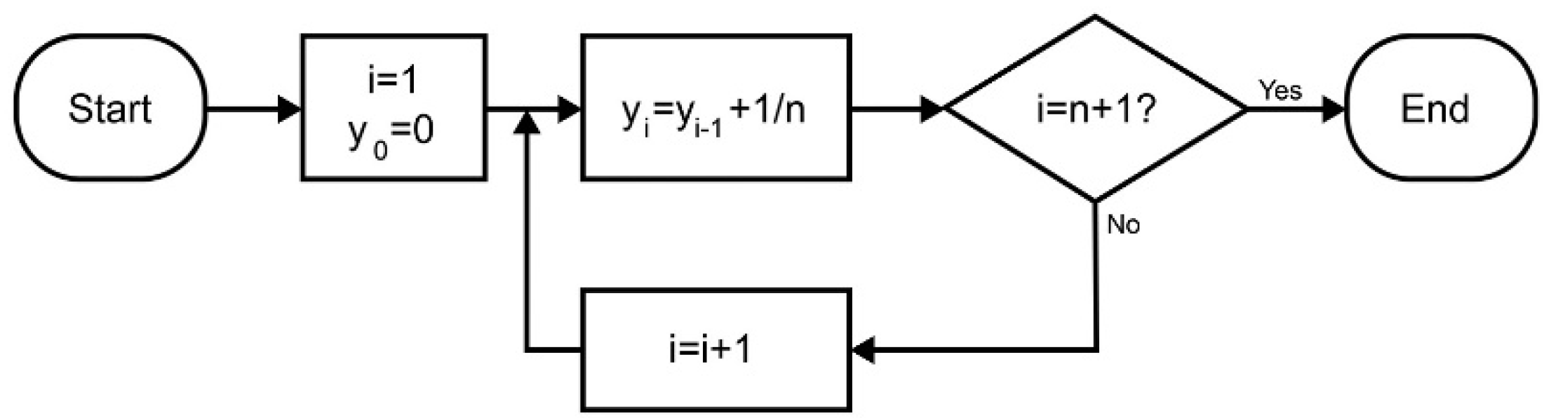
Algorithm distrIN [
1] computes an IN that represents a distribution function
y:
such that
,
. The computation of
is described in
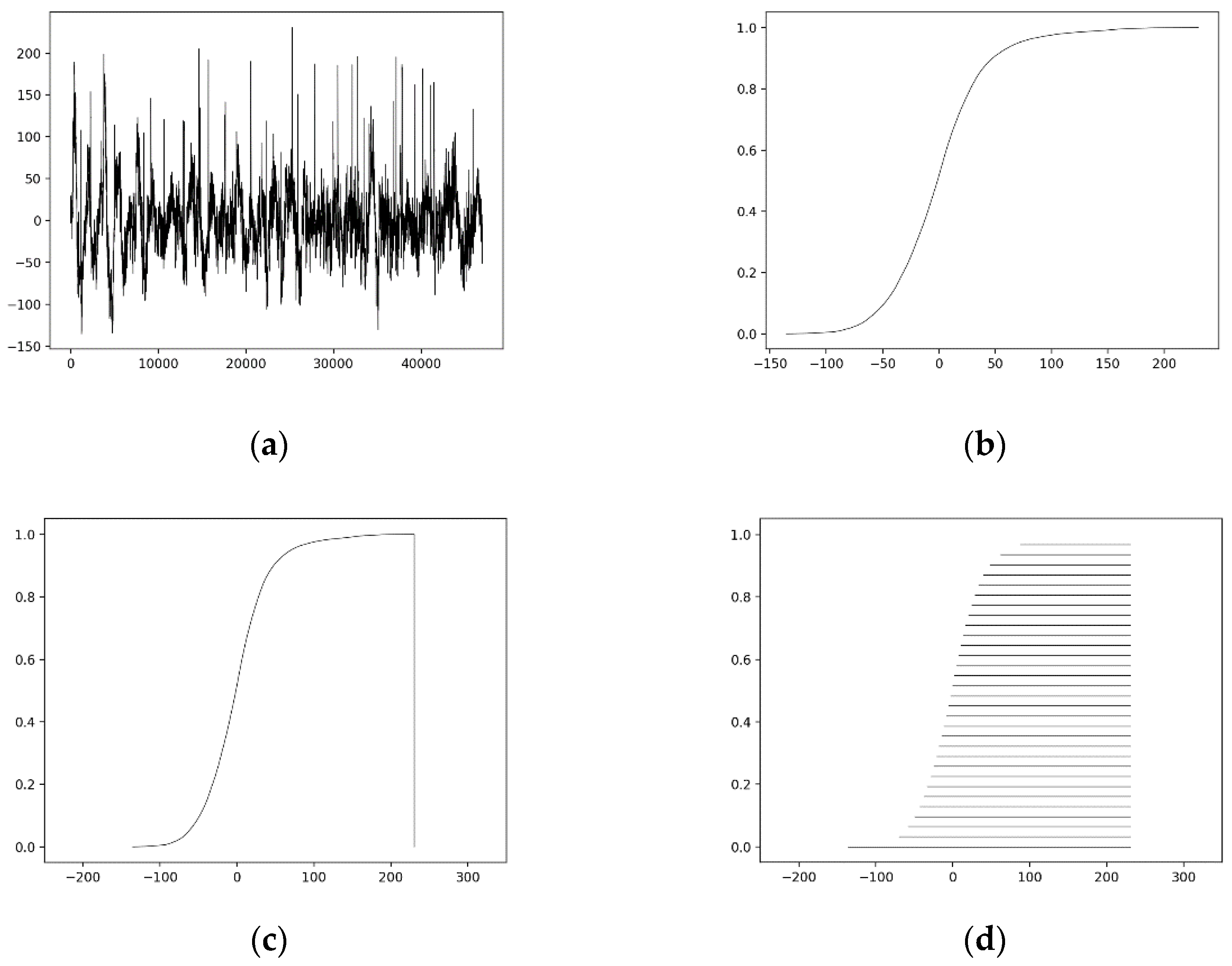
Figure 1 and demonstrated in
Figure 2. In particular,
Figure 2a displays an EEG signal. All the
n + 1 sorted signal values
x0 <
x1 <
x2 < · · · <
xn are input to the distrIN. The corresponding distribution function is shown in
Figure 2b.
Figure 2c shows the computed IN
F in membership-function-representation, whereas
Figure 2d shows the equivalent interval-representation of IN
Fh,
h ∈ [0,1] for 32 levels. It is pointed out that
F1 is always a trivial interval. From the interval-representation, it is clear that an IN is defined by
L intervals with equal rightmost side. An IN represents a distribution of numbers, i.e., potentially orders of magnitude more numbers than
L. The latter is an advantage of INs for big data applications. The main disadvantage of an IN, computed by algorithm distrIN (
Figure 1), is that the “time” dimension of the signal is practically lost. However, the latter is not necessarily catastrophic. For instance, in the proposed study regarding brain signals emotion recognition, an IN considers a signal holistically thus including effectively its emotional content as it is demonstrated experimentally below. Therefore, time here is not critical.
The SEED dataset is employed, which consists of signals acquired by an EEG cap, compatible to the international 10–20 system regarding 62 channels, when 15 subjects watched 15 Chinese movie clips [
46]. The clips were selected so as to elicit either a positive- or neutral- or negative-emotional response. In particular, there were five clips for positive-, five clips for neutral-, and five clips for negative-emotions, respectively. The duration of each film was about 4 min. Each film clip was edited so as to create coherent emotion provocation. In total, there were 15 trials for each experiment. Additionally, the subjects experienced a 5 s hint before each clip, 45 s for self-assessment, and 15 s of rest after each clip. Emotions were extracted via a questionnaire that the subjects had to complete after each clip, following a certain protocol. EEG data were recorded per channel for the duration of each movie clip. Experiments were carried out three times per subject. Hence, for every channel, 3 * 5 * 15 = 225 EEG signals were recorded per emotion. All provided EEGs from SEED datasets are preprocessed, down-sampled to 200 Hz, subjected to a bandpass frequency filter from 0–75 Hz. More details regarding the SEED dataset are provided in [
62]. Each acquired signal was then converted to an IN with
L = 32 levels. It must be highlighted that no further data processing for feature extraction was carried out. To reduce the computational time, the conversion from an EEG signal to an IN was carried out only once, in a data pre-processing step, and the corresponding IN was stored for all future uses.
3.2. Classification
The mathematical background for Fuzzy Lattice Reasoning (FLR) as well as implementation details are presented in [
27]. For two valuation functions
and
θ:
L →
L both fuzzy order functions
σ-meet (
) and
σ-join
can be extended to the lattice (Ι
1,⊑) of intervals, as follows:
Recall that a lattice-order may represent semantics [
31]. In the latter sense, computing in mathematical lattices enables computing with semantics. Here, FLR is engaged for classification by reasoning based on either
or
—recall that any employment of a fuzzy order function (
σ) implements reasoning-by-analogy [
27]. Both parametric functions
θ(.) and
v(.) here are logistic functions:
where
Aν, λν, μν, Cν, Aθ, λθ, μθ, Cθ are eight parameters, i.e., four parameters per function
v(
x) and
θ(
x), to be optimized by a Genetic Algorithm (GA), as detailed below.
To classify a signal according to its emotional content (i.e., positive, neutral or negative), a kNN classifier was engaged using the “leave one out” paradigm, as detailed next.
The data set included 3 * 225 = 675 (EEG) records partitioned in three classes, namely positive, neutral, and negative, with 225 records per class. A record was represented by an N-tuple of Ins, more specifically, one IN was used per channel. Each record, in turn, was left out for testing, whereas all the remaining EEG data records were used for training.
For each “(testing, training)” pair of records, the σ-meet () and σ-join () functions were calculated in two different manners as explained in the following. More specifically, one the one hand, a “single” fuzzy order function, symbolically σ1, was calculated per (testing, training) pair of records. In particular, the numerator was calculated by summing up the corresponding positive valuation function values for all N-tuple IN intervals, likewise, the denominator was calculated. On the other hand, a “many” fuzzy order function, symbolically σ2, was calculated per (testing, training) pair of records as the sum of N individual fuzzy order functions, that is one fuzzy order function was calculated per individual N-tuple entry. In conclusion, four different fuzzy order functions emerged, namely , , , and .
When a new subject was to be tested, then the values for each one of the functions
,
,
, and
were computed for all the training data. The
k largest values identified
k neighbors, which were treated as the
k “nearest neighbors” of a
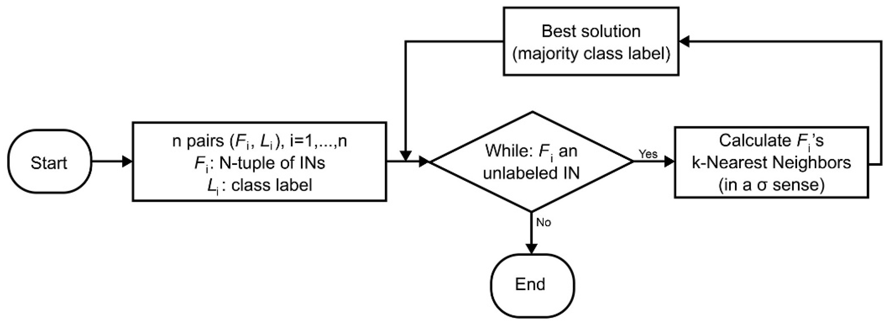
kNN classifier. Nevertheless, it is shown that a conventional
kNN classifier uses a (metric) distance function, whereas the proposed
kNN classifier here uses a fuzzy order function
σ instead. Hence, the proposed classifier’s decisions are based on logic by a fuzzy order function (
σ). The
kNN classification scheme for testing is summarized in
Figure 3. In conclusion, for each fuzzy order function, the classification result was a 3 × 3 confusion matrix
B which stores the percentage of correct classifications for each of the three classes.
3.3. Optimization
To improve the classification performance, a Genetic Algorithm (GA) was engaged towards estimating an optimal set of parameters, as explained in the following.
An initial population of 300 chromosomes was generated such that each chromosome included a set of randomly generated numbers under certain constraints to guarantee that functions
ν(
x) and
θ(
x) are strictly monotonous. More specifically,
ν(
x) is increasing, whereas
θ(
x) is decreasing. For instance, for classification with four channels (i.e., N = 4) each chromosome included 33 parameters. In particular, the first 32 = 8 * 4 parameters specified the fuzzy order functions using eight parameters per pair of INs, i.e., four parameters for each of
ν(
x) and
θ(
x). At the end of a chromosome, one more parameter was added for
k. The overall structure of a chromosome is shown in
Table 1.
The classification result, i.e., a 3 × 3 confusion matrix
Β (classification percentages), was used to compute the cost function as:
To speed up data processing, the chromosomes were partitioned in eight subsets of nearly equal size; next, the evaluation of the aforementioned eight subsets was carried out in parallel. In conclusion, the evaluation of all chromosomes in a subset resulted in a list of costs, which (list) was sorted. Crossover was practiced in each generation with the exchange of randomly selected sets of genes between chromosomes. Mutation was engaged every five generations. In particular, mutation modified 20% of the value of the selected genes of a predefined number of chromosomes. Note that a gene was defined as a set of eight parameters within a chromosome that define the v(x) and θ(x) functions.
4. Experiments, Results, and Discussion
Classification experiments were carried out with five groups of four EEG channels each, i.e., N = 4. The EEG channel selection followed [
34], where five frequency bands (
δ,
θ,
α,
β, and
γ) were computed. Note that for the aforementioned frequency bands, groups of 4, 12, and 20 most significant channels regarding their contribution to emotion classification were identified [
34]. The experiments in this paper were carried out using exclusively the groups G1 to G5 (
Table 2) of four EEG channels [
34]. Note that the groups G1, G2, G3, G4, and G5 correspond to the frequency bands
δ,
θ,
α,
β, and
γ, respectively.
For every group G1, G2, G3, G4, and G5 of channels, an optimization was carried out by a GA. Both fuzzy order functions
σ⨆ and
σ⊓ were used in all combinations with fuzzy order functions
σ1 and
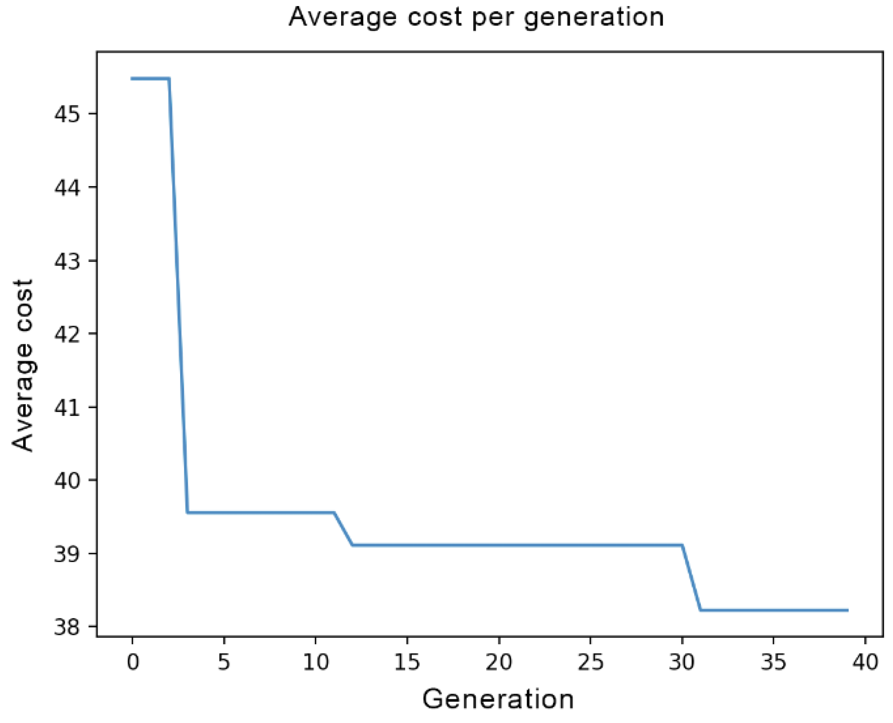
σ2. An optimization task involved 300 chromosomes as the initial population and it was repeated for 40 generations in a row. The number of individuals and the number of generations have been selected empirically. Repeated executions of the optimization algorithm with different parameters did not yield improved classification performance for more generations, the algorithm converged to a solution. Details for both the crossover and the mutation genetic operations were presented in the previous section. In each generation, the best chromosome, i.e., the set of parameters that yielded the best classification result, was stored.
Figure 4 displays a typical example of cost function (5) reduction vs. the number of generations.
For comparison reasons, the same testing and training EEG datasets as in [
34] is employed. Moreover, the leave-one-out cross-validation paradigm is used, as in [
34].
Table 3 displays the results of experiments carried out using a number of channels and state-of-the-art methods from the literature, namely the GSCCA [
34], [
63] (for 4, 12, 20, and 62 channels), a conventional Canonical Correlation Analysis (CCA) method (for 62 channels) [
34], [
64], and a linear SVM classifier (for 62 channels) [
34], [
65]. The proposed classifier
kNN (with
σ) was applied for four channels exclusively.
Table 3 shows that, for four channels,
kNN (with
σ) clearly outperforms GSCCA for all functions
,
,
, and
in all individual frequency bands
δ, θ, α, β, and
γ. In particular, function
outperforms GSCCA in G1, G2, G3, G4, and G5 by 46.13% (from 49.68% to 72.60%), 28.89% (from 57.80% to 74.50%), 28.25% (from 59.57% to 76.40%), 22.34% (from 60.32% to 73.80%), and 19.57% (from 63.56% to 76.00%), respectively. The reason for such a good performance is the unique capacity of
for reasoning beyond an IN’s interval support. It is remarkable that performance drops to 72.90% for
when all frequency bands
δ, θ, α, β, γ are considered jointly in the last column of
Table 3, whereas the corresponding performance of GSCCA peaks to 80.20%.
For
σ1, it turns out that
clearly outperforms
in all individual frequency bands
δ, θ, α, β, and
γ, as it was explained in the previous paragraph, whereas for
σ2, it turns out that
performs better than
in all individual frequency bands. The latter improvement was attributed to the computation of one fuzzy order function per channel. Furthermore, note that the performance peaks to 80.59%, when all frequency bands were considered, surpassing marginally the 80.20% performance of GSCCA. It is pointed out that when all frequency bands were considered then nine individual channels are engaged, namely FT8, FP1, T8, T7, TP7, FC2, PO7, F8, and FPZ, since groups G1 to G5 (
Table 2) do not consider the same four channels.
In our experiments, fuzzy order function
σ1, in particular
, outperforms a fuzzy order function
σ2 on the individual frequency bands
δ, θ, α, and
γ, whereas on frequency band
β it is otherwise. Nevertheless, when all frequency bands are considered then
σ2, in particular
, with 80.59% clearly outperforms
σ1.
Table 3 also shows that the proposed
kNN classifier (for four channels) clearly outperforms alternative classifiers from the literature on individual frequency bands. Nevertheless, when all frequency bands are considered jointly then alternative classifiers, especially for more than four channels, as shown in the last column of
Table 3, may perform better than the proposed
kNN classifier, as explained next.
For ever more channels, as shown in a line of
Table 3, each alternative classifier clearly improves its own performance since it considers incrementally ever more features. For instance, the GSCCA for four channels improves its performance from the interval [49.68%, 63.56%] to 80.20%. However, for more channels, a
kNN (with
σ1) classifier does not increase its own performance substantially. For instance, the proposed
kNN (with
) classifier has produced a slightly better classification result of 69.30% with nine channels since the summation of many terms in both the numerator and the denominator of function
σ1 seems to filter out discriminatory features. Nevertheless, a
kNN (with
σ2) classifier increases its performance since no summation is involved. In particular, the proposed
kNN (with
) classifier has produced a clearly superior classification result of 80.59% with nine channels.
In conclusion, the proposed
kNN (with
σ) classifier has demonstrated superior emotion recognition classification rates in the lower frequency bands
δ, θ, and
α using only four channels compared to alternative classifiers from the literature that use up to 62 channels. However, on the higher frequency bands
β and
γ the proposed
kNN (with
σ) classifier, even though it improves its own performance, performs as well as the alternative classifiers. It is shown that alternative classifiers have improved, even considerably, their own performance when the number of channels was increased, as shown in a line of
Table 3, since they incrementally considered ever more features. The combination of all frequency bands for the proposed method also leads to better results. However, the reported performance of the proposed method outperforms the two out of the five alternative reported methods. In all other cases, it shows similar accuracy as the alternative models. Τhe difference in performance is small, and is offset by the advantages of the proposed method over the existing ones.
Advantages of the proposed kNN (with σ) classifier are summarized in the following. The proposed kNN (with σ) classifier (1) engages raw data represented by INs. In other words, no ad hoc feature extraction is necessary, (2) it has demonstrated a superior capacity for pattern recognition based on parametrically optimizable logic rather than based on a (metric) distance. The capacity of the proposed kNN (with σ) classifier is attributed to the ability of INs to represent all-order data statistics, which are the “features” implicitly involved in the proposed kNN (with σ) classifier.
5. Conclusions and Future Work
This work has introduced a novel scheme for EEG-based emotion recognition, namely “kNN (with σ) classifier” based on logic. The proposed scheme represented an EEG signal by an IN. The aforementioned representation towards emotion recognition is a novelty of this work, which may introduce significant data compression while including potentially all-order data statistics. In addition, no ad hoc feature extraction was needed. Furthermore, tunable nonlinearities can optimize classification performance. Extensive computational experiments using the SEED dataset have demonstrated competitive classification accuracies for the proposed kNN scheme compared to alternative methods from the literature, in particular for four channels. Classification accuracy of up to 80.59% was reported.
A limitation of the proposed method is the loss of “time” dimension. An EEG is a nonstationary signal therefore its distribution changes highly over time. However, the classification performance of the proposed IN-based kNN (with σ) classifier here, has demonstrated that a statistical representation of the signal by an IN, not containing time dimension, could potentially be used to identify the emotional content of an EEG.
Future work would focus on the development and improvement of the existing model for a multiclass classification of emotions. Additionally, future work will consider developing EEG signal processing based on INs using more channels or exploitation of different groups of channels towards enhanced accuracies. Alternative big data applications will also be considered.


 ,
, 


