Adaptive State-Quantized Control of Uncertain Lower-Triangular Nonlinear Systems with Input Delay

Abstract

In this paper, we investigate the adaptive state-quantized control problem of uncertain lower-triangular systems with input delay. It is assumed that all state variables are quantized for the feedback control design. The error transformation method using an auxiliary time-varying signal is presented to deal with the compensation problem of input delay. Based on the error surfaces with the auxiliary variable, a neural-network-based adaptive state-quantized control scheme is constructed with the design of the input delay compensator. Different from existing results in the literature, the proposed method exhibits the following features: (i) compensating for the input delay effect by using quantized states; and (ii) establishing the stability of the adaptive quantized feedback control system in the presence of input delay. Furthermore, the boundedness of all the signals in the closed-loop and the convergence of the tracking error are analyzed. The effectiveness of the developed control strategy is demonstrated through the simulation on a hydraulic servo system.

1. Introduction

Owing to theoretical challenges and several practical applications, the feedback control problems of triangular nonlinear systems have been actively addressed in the control community (see [1,2,3] and references therein). Especially, as network-based industrial applications increase, input delays caused by the network transformation become unavoidable in the control system [4,5]. Therefore, the control design strategies for uncertain nonlinear systems with input delay have been developed. In [6,7,8,9], predictor-based control approaches are presented for nonlinear systems with input delay. A truncated-predictor-based control method has been studied for nonlinear systems with Lipschitz nonlinearities [10]. However, these results [6,7,8,9,10] only consider uncertain nonlinearities matched to the delayed control input. To deal with uncertain nonlinearities unmatched to the delayed control input, adaptive control design strategies using Pade approximation have been developed for uncertain triangular nonlinear systems with input delay [11,12,13,14]. In [15,16,17,18,19], input delay compensation approaches using the high-order auxiliary dynamics are presented to eliminate the influence of input delay on the recursive controller design. However, these studies do not consider the state quantization problem that is important with the input delay problem in network-based control environments with the communication channel bandwidth and limited computation resources. To the best of our knowledge, the state-quantized control problem of uncertain lower-triangular systems with input delay is still open.

The quantized control problem under capability-limited communication network is attracting much research attention recently, owing to extensive industrial applications [20,21]. To overcome the capability-limited communication problem, the quantization of all measured state variables is required to transmit state-feedback signals to the controller through the network. In this procedure, the quantization errors in the closed-loop cause control performance degradation and even instability. Motivated by the above-mentioned issues, state-quantized control methods have been proposed for lower-triangular nonlinear systems with Lipchitz conditions [22,23]. To approximate unknown and unmatched nonlinearities in nonlinear systems, a neural-network-based quantized feedback control result is presented in [24]. This approach has been extended to nonlinear strict-feedback systems with state delays [25] where the Lyapunov–Krasovskii functional technique is employed to remove the effects of state delays. Despite these studies, the input delay problem has not been investigated in the quantized feedback control framework of triangular nonlinear systems. The main difficulty in dealing with input delay in the state-quantized control design is to provide the input delay compensator using quantized states and to analyze the stability of the closed-loop signals including the input delay compensator.

In this paper, we aim at addressing the adaptive state-quantized control problem in the presence of input delay in uncertain triangular nonlinear systems with unknown nonlinearities and external disturbances. The measured full states are quantized by state quantizers and the quantized states are only used to design the controller. Different from the existing quantized feedback control results [22,23,24,25], our primary contribution is to establish an input delay compensation strategy using quantized states in the state-quantized control framework while ensuring the robustness against unknown nonlinearities and external disturbances. To this end, an error coordinated transformation using the auxiliary variable is derived to design the delay compensator and the neural-network-based adaptive controller. An adaptive state-quantized control scheme is designed to guarantee the boundedness of all involved signals and the quantization errors. In the proposed control structure, the delay compensator and adaptive tuning laws based on quantized states are induced from the Lyapunov-based stability analysis methodology. It is shown that the control error is guaranteed to converge to a set that can be reduced as small as desired by adjusting design parameters. The simulation result on a hydraulic servo system is provided to demonstrate the effectiveness of the developed theoretical strategy.

The paper is organized as follows. In Section 2, the state-quantized control problem in the presence of input delay is formulated and the neural network approximation property is introduced. In Section 3, the adaptive state-quantized control scheme with a delay compensator and its closed-loop stability analysis are given. In Section 4, the simulation result on a hydraulic servo system is presented to illustrate the effectiveness of the state-quantized control scheme. Finally, the paper is concluded in Section 5.

2. Problem Formulation

In this paper, we consider the following class of uncertain lower-triangular nonlinear systems with input delay:

$$\begin{array}{c}\hfill \begin{array}{c}{\dot{x}}_i\left(t\right)=x_{i+1}\left(t\right)+g_i\left({\overline{x}}_i\left(t\right)\right)+{\delta }_i\left(t\right)\hfill \\ {\dot{x}}_n\left(t\right)=u(t-d)+g_n\left({\overline{x}}_n\left(t\right)\right)+{\delta }_n\left(t\right)\hfill \\ y\left(t\right)=x_1\left(t\right)\hfill \end{array}\end{array}$$

(1)

where $i=1,\dots ,n-1$, ${\overline{x}}_j=[x_1,\dots ,x_j]\in {\mathbb{R}}^j$, $j=1,\dots ,n$, are the state variable vectors, $y\in \mathbb{R}$ denotes the system output, d is a non-negative input delay, $u(t-d)\in \mathbb{R}$ is the control input with input delay, ${\delta }_j$, $j=1,\dots ,n$, are uncertain exogenous disturbances, and $g_j\left({\overline{x}}_j\right):{\mathbb{R}}^j\mapsto \mathbb{R}$, $j=1,\dots ,n$, are unknown $C^1$ nonlinear functions. The networked-based control problem with state quantization is considered in this paper. Then, all state variables $x_j$, $j=1,\dots ,n$, are quantized via the following uniform quantizer

$$\begin{array}{c}\hfill Q\left(x_j\right)=\left\{\begin{array}{c}{\rho }_l,{\rho }_l-\frac{\omega }{2}\le x_j<{\rho }_l+\frac{\omega }{2}\hfill \\ 0,-\frac{\omega }{2}\le x_j<\frac{\omega }{2}\hfill \\ -{\rho }_l,-{\rho }_l-\frac{\omega }{2}\le x_j<-{\rho }_l+\frac{\omega }{2}\hfill \end{array}\right.\end{array}$$

(2)

where $j=1,\dots ,n$, $l\in {\mathbb{Z}}^{+}$, $\omega$ is the quantization level, ${\rho }_1=\omega$, and ${\rho }_{l+1}={\rho }_l+\omega$. Then, the quantization error is defined as ${\zeta }_{x_j}\triangleq x_j-Q\left(x_j\right)$ that satisfies the property $|{\zeta }_{x_j}|\le \omega$ [26]. Thus, $Q\left(x_j\right)$ instead of $x_j$ are available for the design of the feedback control law u where $j=1,\dots ,n$.

The main objective of this paper is to design an adaptive tracking law u using quantized states $Q\left(x_j\right)$ for nonlinear systems (1) with input delay so that the system output y follows the desired signal $y_r$ while all the closed-loop signals remain bounded where $y_r$, ${\dot{y}}_r$, and ${\ddot{y}}_r$ are bounded.

Assumption 1.

The disturbances ${\delta }_j$ are bounded as $|{\delta }_j|\le {\overline{\delta }}_j$ where $j=1,\dots ,n$ and ${\overline{\delta }}_j$ are unknown constants.

In the proposed control scheme, the unknown nonlinear functions $g_j$, $j=1,\dots ,n$, are online approximated via the radial basis function neural networks (RBFNNs) over compact sets ${\Xi }_j\subset {\mathbb{R}}^j$ as follows [27]:

$$\begin{array}{cc}\hfill g_j\left({\overline{x}}_j\right)& ={\Theta }_j^{\top }{B}_j\left({\overline{x}}_j\right)+{\epsilon }_j\left({\overline{x}}_j\right)\hfill \end{array}$$

(3)

where ${\overline{x}}_j\in {\Xi }_j$ denotes an input vector, ${\Theta }_j\in {\mathbb{R}}^N$ is an ideal bounded weighting vector satisfying $\parallel {\Theta }_j\parallel \le {\overline{\Theta }}_j$ with a constant ${\overline{\Theta }}_j$, ${\epsilon }_j$ denotes a reconstruction error satisfying $|{\epsilon }_j|\le {\overline{\epsilon }}_j$ with a constant ${\overline{\epsilon }}_j$, and $B_j={[b_{j,1},\dots ,b_{j,N}]}^{\top }\in {\mathbb{R}}^N$ is the Gaussian function vector with elements $b_{j,m}\left({\overline{x}}_j\right)=e^{-{\parallel {\overline{x}}_j-c_{j,m}\parallel }^2/w_{j,m}^2}$, $m=1,\dots ,N$. Here, $c_{j,m}\in {\mathbb{R}}^j$ and $w_{j,m}$ are the center and width of the Gaussian functions, respectively.

Lemma 1.

[28,29] The Gaussian basis function vector $B_j$ is bounded as $\parallel B_j\parallel \le {\overline{B}}_j$ with a constant ${\overline{B}}_j$.

3. Adaptive State-Quantized Tracking Control in the Presence of Input Delay

In this section, we design the neural-network-based adaptive state-quantized controller using the following coordinated transformation:

$$\begin{array}{c}\hfill \begin{array}{c}{s}_1=y-y_r\hfill \\ s_i=x_i-{\beta }_{i-1,1},i=2,\dots ,n-1\hfill \\ s_n=x_n-{\beta }_{n-1,1}-k_{u}tanh\rho \hfill \\ {\tilde{\beta }}_{m,1}={\beta }_{m,1}-v_m,m=1,\dots ,n-1\hfill \end{array}\end{array}$$

(4)

where $s_j$, $j=1,\dots ,n$, denote error surfaces, $k_u>0$ is a design parameter, $\rho$ is the auxiliary time-varying signal for compensating for the input delay effect, $v_m$ are virtual controllers, and ${\beta }_{m,1}$ are the signals obtained by the following low-pass command filters

$$\begin{array}{c}\hfill \begin{array}{c}{\dot{\beta }}_{m,1}={\beta }_{m,2}\hfill \\ {\dot{\beta }}_{m,2}=-2a_{m,1}{a}_{m,2}{\beta }_{m,2}-a_{m,2}^2({\beta }_{m,1}-v_m)\hfill \end{array}\end{array}$$

(5)

where ${\beta }_{m,1}\left(0\right)=v_m\left(0\right)$, ${\beta }_{m,2}\left(0\right)=0$, and $a_{m,1}>0$ and $a_{m,1}>0$ are design constants. Notice that the command filters (5) are employed based on the command filtered backstepping approach [3].

Remark 1.

Compared with the existing adaptive control works for state-quantized nonlinear systems [22,23,24,25], this paper presents the error transformation method using the auxiliary variable ρ to deal with the input delay problem in the quantized feedback control framework. We design the input delay compensator using quantized states at the last design step and the stability analysis strategy of the total closed-loop system including this input delay compensator is presented in this paper. This is the main contribution of our study.

The controller design is presented from the Lyapunov-based recursive design step by step.

Step 1: Using (1) and (4), the dynamics of $s_1$ is defined as ${\dot{s}}_1=x_2+g_1+{\delta }_1-{\dot{y}}_r$. By considering a Lyapunov function $V_1=(1/2)s_1^2$ and using (3), we have

$$\begin{array}{cc}\hfill {\dot{V}}_1& =s_1[s_2+{\tilde{\beta }}_{1,1}+v_1+{\Theta }_1^{\top }{B}_1\left(x_1\right)+{\epsilon }_1+{\delta }_1-{\dot{y}}_r].\hfill \end{array}$$

(6)

Then, we choose the virtual control law $v_1$ as

$$\begin{array}{cc}\hfill v_1& =-k_1{s}_1-{\widehat{\Theta }}_1^{\top }{B}_1\left(x_1\right)-{\widehat{\gamma }}_{1}tanh\left(\frac{s_1}{{\sigma }_1}\right)+{\dot{y}}_r\hfill \end{array}$$

(7)

where $k_1>0$ and ${\sigma }_1>0$ denote design constants, ${\widehat{\Theta }}_1$ is the estimate of ${\Theta }_1$, and ${\widehat{\gamma }}_1$ is the estimate of the unknown parameter ${\overline{\gamma }}_1$ to be determined later.

Using (7), (6) becomes

$$\begin{array}{cc}\hfill {\dot{V}}_1& =-k_1{s}_1^2-s_1{\tilde{\Theta }}_1^{\top }{B}_1\left(x_1\right)-s_1{\widehat{\gamma }}_{1}tanh\left(\frac{s_1}{{\sigma }_1}\right)+s_1(s_2+{\tilde{\beta }}_{1,1}+{\epsilon }_1+{\delta }_1)\hfill \end{array}$$

(8)

where ${\tilde{\Theta }}_1={\widehat{\Theta }}_1-{\Theta }_1$ is an estimation error vector.

Step i $(i=2,\dots ,n-1)$: Consider the Lyapunov function $V_i=(1/2)s_i^2$. Using (3)–(5), the time derivative of $V_i$ is represented by

$$\begin{array}{cc}\hfill {\dot{V}}_i& =s_i(s_{i+1}+{\tilde{\beta }}_{i,1}+v_i+{\Theta }_i^{\top }{B}_i\left({\overline{x}}_i\right)+{\epsilon }_i+{\delta }_i-{\beta }_{i-1,2}).\hfill \end{array}$$

(9)

The virtual control law $v_i$ is designed as

$$\begin{array}{cc}\hfill v_i& =-k_i{s}_i-{\widehat{\Theta }}_i^{\top }{B}_i\left({\overline{x}}_i\right)-{\widehat{\gamma }}_{i}tanh\left(\frac{s_i}{{\sigma }_i}\right)+{\beta }_{i-1,2}\hfill \end{array}$$

(10)

where $k_i>0$ and ${\sigma }_i>0$ denote design constants, ${\widehat{\Theta }}_i$ is the estimate of ${\Theta }_i$, and ${\widehat{\gamma }}_i$ is the estimate of ${\overline{\gamma }}_i$ to be constructed later.

Using (10), (9) is obtained as

$$\begin{array}{cc}\hfill {\dot{V}}_i& =-k_i{s}_i^2-s_i{\tilde{\Theta }}_i^{\top }{B}_i\left({\overline{x}}_i\right)-{\widehat{\gamma }}_{i}tanh\left(\frac{s_i}{{\sigma }_i}\right)+s_i(s_{i+1}+{\tilde{\beta }}_{i,1}+{\epsilon }_i+{\delta }_i)\hfill \end{array}$$

(11)

where ${\tilde{\Theta }}_i={\widehat{\Theta }}_i-{\Theta }_i$ is an estimation error vector.

Step n: A Lyapunov function is defined as $V_n=(1/2)s_n^2$. Using (3)–(5), the time derivative of $V_n$ is represented by

$$\begin{array}{cc}\hfill {\dot{V}}_n& =s_n(u(t-d)+{\Theta }_n^{\top }{B}_n\left({\overline{x}}_n\right)+{\epsilon }_n+{\delta }_n-{\beta }_{n-1,2}-k_u{\left({cosh}^2\rho \right)}^{-1}\dot{\rho }).\hfill \end{array}$$

(12)

The input delay compensator is designed as

$$\begin{array}{c}\hfill \dot{\rho }=\frac{{cosh}^2\rho }{k_u}(-ptanh\rho +u(t-d)-u\left(t\right))\end{array}$$

(13)

where $p>0$ is a design constant.

Substituting (13) into (12) and defining an un-quantized control signal $v_n$, we have

$$\begin{array}{cc}\hfill {\dot{V}}_n& =s_n(u\left(t\right)-v_n)+s_n(v_n+{\Theta }_n^{\top }{B}_n\left({\overline{x}}_n\right)+{\epsilon }_n+{\delta }_n-{\beta }_{n-1,2}+ptanh\rho ).\hfill \end{array}$$

(14)

Then, $v_n$ is selected as

$$\begin{array}{c}\hfill v_n=-k_n{s}_n-{\widehat{\Theta }}_n^{\top }{B}_n\left({\overline{x}}_n\right)-{\widehat{\gamma }}_{n}tanh\left(\frac{s_n}{{\sigma }_n}\right)+{\beta }_{n-1,2}\end{array}$$

(15)

where $k_n>0$ and ${\sigma }_n>0$ denote design constants, ${\widehat{\Theta }}_n$ is the estimate of ${\Theta }_n$, and ${\widehat{\gamma }}_n$ is the estimate of ${\overline{\gamma }}_n$ to be constructed later.

Applying (15) into (14) yields

$$\begin{array}{cc}\hfill {\dot{V}}_n& =-k_n{s}_n^2-{\tilde{\Theta }}_n^{\top }{B}_n\left({\overline{x}}_n\right)-{\widehat{\gamma }}_{n}tanh\left(\frac{s_n}{{\sigma }_n}\right)+s_n(u\left(t\right)-v_n)+s_n({\epsilon }_n+{\delta }_n+ptanh\rho )\hfill \end{array}$$

(16)

where ${\tilde{\Theta }}_n={\widehat{\Theta }}_n-{\Theta }_n$ is an estimation error vector.

For the design of the adaptive state-quantized control law u, we define error surfaces $s_{q,j}$, $j=1,\dots ,n$, using quantized states $Q\left(x_j\right)$ as

$$\begin{array}{c}\hfill \begin{array}{c}{s}_{q,1}=Q\left(x_1\right)-y_r\hfill \\ s_{q,i}=Q\left(x_i\right)-{\beta }_{q,i-1,1},i=2,\dots ,n-1\hfill \\ s_{q,n}=Q\left(x_n\right)-{\beta }_{q,n-1,1}-k_{u}tanh\rho \hfill \end{array}\end{array}$$

(17)

where ${\beta }_{q,i-1,1}$ and ${\beta }_{q,n-1,1}$ are the command filtered signals of state-quantized virtual controllers $v_{q,i-1}$ and $v_{q,n-1}$, respectively, and $\rho$ is obtained using the input delay compensator (13). The state-quantized virtual controllers $v_{q,m}$ and actual controller u are designed as

$$\begin{array}{cc}\hfill v_{q,m}& =-k_m{s}_{q,m}-{\widehat{\Theta }}_m^{\top }{B}_m\left(Q\left({\overline{x}}_m\right)\right)-{\widehat{\gamma }}_{m}tanh\left(\frac{s_{q,m}}{{\sigma }_m}\right)+{\beta }_{q,m-1,2}\hfill \end{array}$$

(18)

$$\begin{array}{cc}\hfill u& =-k_n{s}_{q,n}-{\widehat{\Theta }}_n^{\top }{B}_n\left(Q\left({\overline{x}}_n\right)\right)-{\widehat{\gamma }}_{n}tanh\left(\frac{s_{q,n}}{{\sigma }_n}\right)+{\beta }_{q,n-1,2}\hfill \end{array}$$

(19)

where $m=1,\dots ,n-1$, $Q\left({\overline{x}}_j\right)={[Q\left(x_1\right),\dots ,Q\left(x_j\right)]}^{\top }$, $j=1,\dots ,n$, ${\beta }_{q,0,2}={\dot{y}}_r$, and the adaptive laws for ${\widehat{\Theta }}_j$ and ${\widehat{\gamma }}_j$ are constructed as

$$\begin{array}{cc}\hfill {\dot{\widehat{\Theta }}}_j& ={\lambda }_{\Theta ,j}[s_{q,j}{B}_j\left(Q\left({\overline{x}}_j\right)\right)-{\sigma }_{\Theta ,j}|s_{q,j}\left|{\widehat{\Theta }}_j\right]\hfill \end{array}$$

(20)

$$\begin{array}{cc}\hfill {\dot{\widehat{\gamma }}}_j& ={\lambda }_{\gamma ,j}\left[s_{q,j}tanh\left(\frac{s_{q,j}}{{\sigma }_j}\right)-{\sigma }_{\gamma ,j}\left|s_{q,j}\right|{\widehat{\gamma }}_j\right]\hfill \end{array}$$

(21)

with $j=1,\dots ,n$, tuning matrices ${\lambda }_{\Theta ,j}>0$, tuning gains ${\lambda }_{\gamma ,j}>0$, and positive constants ${\sigma }_{\Theta ,j}$ and ${\sigma }_{\gamma ,j}$ for $\sigma -$ modification. Here, based on (5), the command filters for ${\beta }_{q,m,1}$ and ${\beta }_{q,m,2}$ are designed as

$$\begin{array}{c}\hfill \begin{array}{c}{\dot{\beta }}_{q,m,1}={\beta }_{q,m,2}\hfill \\ {\dot{\beta }}_{q,m,2}=-2a_{m,1}{a}_{m,2}{\beta }_{q,m,2}-a_{m,2}^2({\beta }_{q,m,1}-v_{q,m})\hfill \end{array}\end{array}$$

(22)

where $m=1,\dots ,n-1$, ${\beta }_{q,m,1}\left(0\right)=v_{q,m}\left(0\right)$, and ${\beta }_{q,m,2}\left(0\right)=0$.

Remark 2.

The proposed adaptive state-quantized control scheme consists of the virtual and actual controllers (18) and (19) with the delay compensator (13), adaptive laws (20) and (21), and command filter (22) using the quantized states $Q\left(x_j\right)$, $j=1,\dots ,n$. Compared with the existing control works for nonlinear lower-triangular systems with input delay [11,12,13,14,15,16,17,18,19], the state quantization problem is firstly considered in this paper. Thus, the stability analysis strategy of the closed-loop systems with the proposed adaptive state-quantized control scheme in the presence of input delay should be newly presented.

For the stability analysis, we present the following lemmas.

Lemma 2.

If ${\widehat{\Theta }}_j$ and ${\widehat{\gamma }}_j$ are tuned via the adaptive laws (20) and (21), respectively, then: (i) ${\tilde{\Theta }}_j\left(t\right)\in {\Pi }_{\Theta ,j}$, $\forall t\ge 0$, is ensured when ${\tilde{\Theta }}_j\left(0\right)\in {\Pi }_{\Theta ,j}$; and (ii) ${\tilde{\gamma }}_j\left(t\right)\in {\Pi }_{\gamma ,j}$, $\forall t\ge 0$, is ensured when ${\tilde{\gamma }}_j\left(0\right)\in {\Pi }_{\gamma ,j}$ where $j=1,\dots ,n$, ${\Pi }_{\Theta ,j}=\{{\tilde{\Theta }}_j|\parallel {\tilde{\Theta }}_j\parallel \le {\psi }_{\Theta ,j}\}$ with a constant ${\psi }_{\Theta ,j}$, ${\tilde{\gamma }}_j={\widehat{\gamma }}_j-{\overline{\gamma }}_j$, and ${\Pi }_{\gamma ,j}=\{{\tilde{\gamma }}_j\left|\right|{\tilde{\gamma }}_j|\le {\psi }_{\gamma ,j}\}$ with a constant ${\psi }_{\gamma ,j}$.

Proof. 

(i) A Lyapunov function $V_{\Theta ,j}=(1/2){\tilde{\Theta }}_j^{\top }{\lambda }_{\Theta ,j}^{-1}{\tilde{\Theta }}_j$ is considered. Then, differentiating $V_{\Theta ,j}$ with respect to time and using ${\widehat{\Theta }}_j={\Theta }_j+{\tilde{\Theta }}_j$, we have

$$\begin{array}{cc}\hfill {\dot{V}}_{\Theta ,j}& ={\tilde{\Theta }}_j^{\top }(s_{q,j}{B}_j\left(Q\left({\overline{x}}_j\right)\right)-{\sigma }_{\Theta ,j}|s_{q,j}\left|({\Theta }_j+{\tilde{\Theta }}_j)\right).\hfill \end{array}$$

(23)

Using $\parallel {\Theta }_j\parallel \le {\overline{\Theta }}_j$ and Lemma 1, we obtain

$$\begin{array}{cc}\hfill {\dot{V}}_{\Theta ,j}& \le \parallel {\tilde{\Theta }}_j\parallel |s_{q,j}\left|\right({\overline{B}}_j+{\sigma }_{\Theta ,j}{\overline{\Theta }}_j-{\sigma }_{\Theta ,j}\parallel {\tilde{\Theta }}_j\parallel ).\hfill \end{array}$$

(24)

Then, it is ensured that ${\dot{V}}_{\Theta ,j}\le 0$ when $\parallel {\tilde{\Theta }}_j\parallel \ge {\psi }_{\Theta ,j}$ with ${\psi }_{\Theta ,j}=({\overline{B}}_j+{\sigma }_{\Theta ,j}{\overline{\Theta }}_j)/{\sigma }_{\Theta ,j}$. Thus, when ${\tilde{\Theta }}_j\left(0\right)\in {\Pi }_{\Theta ,j}$, ${\tilde{\Theta }}_j\left(t\right)\in {\Pi }_{\Theta ,j}$, $\forall t\ge 0$, is ensured.

(ii) By defining a Lyapunov function $V_{\gamma ,j}=(1/\left(2{\lambda }_{\gamma ,j}\right)){\tilde{\gamma }}_j^2$ and using ${\widehat{\gamma }}_j={\overline{\gamma }}_j+{\tilde{\gamma }}_j$ and the property $|tanh(·\left)\right|\le 1$, the time derivative of $V_{\gamma ,j}$ is

$$\begin{array}{cc}\hfill {\dot{V}}_{\gamma ,j}& \le |{\tilde{\gamma }}_j\left|\right|s_{q,j}\left|\right(1+{\sigma }_{\gamma ,j}{\overline{\gamma }}_j-{\sigma }_{\gamma ,j}|{\tilde{\gamma }}_j\left|\right).\hfill \end{array}$$

(25)

By defining ${\psi }_{\gamma ,j}\triangleq (1+{\sigma }_{\gamma ,i}{\overline{\gamma }}_j)/{\sigma }_{\gamma ,j}$, we know that ${\dot{V}}_{\gamma ,j}\le 0$ when $|{\tilde{\gamma }}_j|\ge {\psi }_{\gamma ,j}$. Thus, ${\tilde{\gamma }}_j\left(t\right)\in {\Pi }_{\gamma ,j}$ is ensured for all $t\ge 0$ provided that ${\tilde{\gamma }}_j\left(0\right)\in {\Pi }_{\gamma ,j}$. ☐

Lemma 3.

Let us define the errors between the un-quantized signals and quantized signals in the closed-loop system as ${\zeta }_{s,j}=s_j-s_{q,j}$, ${\zeta }_{v,i}=v_i-v_{q,i}$, ${\zeta }_u=v_n-u$, ${\zeta }_{\beta ,i,1}={\beta }_{i,1}-{\beta }_{q,i,1}$, and ${\zeta }_{\beta ,i,2}={\beta }_{i,2}-{\beta }_{q,i,2}$ where $j=1,\dots ,n$ and $i=1,\dots ,n-1$. Then, these errors are bounded as $|{\zeta }_{s,j}|\le {\chi }_{s,j}$, $|{\zeta }_{v,i}|\le {\chi }_{v,i}$, $|{\zeta }_u|\le {\chi }_u$ and $\parallel {\zeta }_{\beta ,i}\parallel \le {\chi }_{\beta ,i}$ where ${\zeta }_{\beta ,i}={[{\zeta }_{\beta ,i,1},{\zeta }_{\beta ,i,2}]}^{\top }$, and ${\chi }_{s,j}$, ${\chi }_{v,i}$, and ${\chi }_{\beta ,i}$ are constants.

Proof. 

We prove the boundedness of the quantization errors step by step.

(i) From $|x_1-Q\left(x_1\right)|\le \omega$ and ${\zeta }_{s,1}=s_1-s_{q,1}=x_1-Q\left(x_1\right)$, we have $|{\zeta }_{s,1}|\le {\chi }_{s,1}\triangleq \omega$. Then, using (7) and (18), ${\zeta }_{v,1}$ becomes

$$\begin{array}{c}\hfill {\zeta }_{v,1}=-k_1{\zeta }_{s,1}-{\widehat{\Theta }}_1^{\top }(B_1\left(x_1\right)-B_1\left(Q\left(x_1\right)\right))-{\widehat{\gamma }}_1\left[tanh\left(\frac{s_1}{{\sigma }_1}\right)-tanh\left(\frac{s_{q,1}}{{\sigma }_1}\right)\right].\end{array}$$

(26)

From Lemma 1 and $|tanh(·\left)\right|\le 1$, we have $|B_1\left(x_1\right)-B_1\left(Q\left(x_1\right)\right)|\le 2{\overline{B}}_1$ and $|tanh(s_1/{\sigma }_1)-tanh(s_{q,1}/{\sigma }_1)|\le 2$. Then, using Lemma 2, it is ensured that $\parallel {\widehat{\Theta }}_1\parallel \le {\psi }_{\Theta ,1}+{\overline{\Theta }}_1$ and $|{\widehat{\gamma }}_1|\le {\psi }_{\gamma ,1}+{\overline{\gamma }}_1$. Thus, ${\zeta }_{v,1}$ is bounded as $|{\zeta }_{v,1}|\le {\chi }_{v,1}$ with ${\chi }_{v,1}=k_1{\chi }_{s,1}+2{\overline{B}}_1({\psi }_{\Theta ,1}+{\overline{\Theta }}_1)+2({\psi }_{\gamma ,1}+{\overline{\gamma }}_1)$.

The vector forms of the command filters (5) and (22) are written as

$$\begin{array}{c}\hfill {\dot{\beta }}_1={\Gamma }_1{\beta }_1+{\Delta }_1{v}_1,{\dot{\beta }}_{q,1}={\Gamma }_1{\beta }_{q,1}+{\Delta }_1{v}_{q,1}\end{array}$$

(27)

where ${\beta }_1={[{\beta }_{1,1},{\beta }_{1,2}]}^{\top }$, ${\beta }_{q,1}={[{\beta }_{q,1,1},{\beta }_{q,1,2}]}^{\top }$, ${\Gamma }_1=\left[\begin{array}{cc}0& 1\\ -a_{1,2}^2& -2a_{1,1}{a}_{1,2}\end{array}\right]$, and ${\Delta }_1={[0,a_{1,2}^2]}^{\top }$. Thus, we have

$$\begin{array}{c}\hfill {\dot{\zeta }}_{\beta ,1}={\Gamma }_1{\zeta }_{\beta ,1}+{\Delta }_1{\zeta }_{v,1}.\end{array}$$

(28)

The solution of (28) is represented by

$$\begin{array}{cc}\hfill {\zeta }_{\beta ,1}\left(t\right)& =e^{{\Gamma }_{1}t}{\zeta }_{\beta ,1}\left(0\right)+{\int }_0^t{e}^{{\Gamma }_1(t-\tau )}{\Delta }_1{\zeta }_{v,1}\left(\tau \right)d\tau .\hfill \end{array}$$

(29)

Using $|{\zeta }_{v,1}|\le {\chi }_{v,1}$, the invertible property of $A_1$, and the inequality $\parallel e^{{\Gamma }_{1}t}\parallel \le {\iota }_{1,1}{e}^{-{\iota }_{1,2}t}$ with constants ${\iota }_{1,1}>0$ and ${\iota }_{1,2}>0$ [30], ${\zeta }_{\beta ,1}$ is bounded as

$$\begin{array}{cc}\hfill \parallel {\zeta }_{\beta ,1}\left(t\right)\parallel & \le {\iota }_{1,1}\parallel {\zeta }_{\beta ,1}\left(0\right)\parallel +{\chi }_{v,1}\parallel {\Delta }_1\parallel \parallel {\Gamma }_1^{-1}(I-e^{{\Gamma }_{1}t})\parallel \hfill \\ \hfill & \le {\chi }_{\beta ,1}\hfill \end{array}$$

(30)

where ${\chi }_{\beta ,1}={\iota }_{1,1}\parallel {\zeta }_{\beta ,1}\left(0\right)\parallel +{\chi }_{v,1}\parallel {\Delta }_1\parallel \parallel {\Gamma }_1^{-1}\parallel (1+{\iota }_{1,1})\parallel$.

(ii) Using (4) and (17), we have ${\zeta }_{s,i}=x_i-Q\left(x_i\right)+{\zeta }_{\beta ,i-1,1}$ where $i=2,\dots ,n-1$. From $|x_i-Q\left(x_i\right)|\le \omega$ and $|{\zeta }_{\beta ,i-1,1}|\le {\chi }_{\beta ,i-1}$, ${\zeta }_{s,i}$ is bounded as $|{\zeta }_{s,i}|\le {\chi }_{s,i}\triangleq \omega +{\chi }_{\beta ,i-1}$. Then, ${\zeta }_{v,i}$ is given by

$$\begin{array}{c}\hfill {\zeta }_{v,i}=-k_i{\zeta }_{s,i}-{\widehat{\Theta }}_i^{\top }(B_i\left({\overline{x}}_i\right)-B_i\left(Q\left({\overline{x}}_i\right)\right))-{\widehat{\gamma }}_i\left[tanh\left(\frac{s_i}{{\sigma }_i}\right)-tanh\left(\frac{s_{q,i}}{{\sigma }_i}\right)\right]+{\zeta }_{\beta ,i-1,2}.\end{array}$$

(31)

From the procedure similar to the previous step and $|{\zeta }_{\beta ,i-1,2}|\le {\chi }_{\beta ,i-1}$, ${\zeta }_{v,i}$ is bounded as $|{\zeta }_{v,i}|\le {\chi }_{v,i}$ with ${\chi }_{v,i}=k_i{\chi }_{s,i}+2{\overline{B}}_i({\psi }_{\Theta ,i}+{\overline{\Theta }}_i)+2({\psi }_{\gamma ,i}+{\overline{\gamma }}_i)+{\chi }_{\beta ,i-1}$.

By applying the procedures (29) and (30) to ${\dot{\zeta }}_{\beta ,i}={\Gamma }_i{\zeta }_{\beta ,i}+{\Delta }_i{\zeta }_{v,i}$, and using the inequality $\parallel e^{{\Gamma }_{i}t}\parallel \le {\iota }_{i,1}{e}^{-{\iota }_{i,2}t}$ with constants ${\iota }_{i,1}>0$ and ${\iota }_{i,2}>0$, we have $\parallel {\zeta }_{\beta ,i}\left(t\right)\parallel \le {\chi }_{\beta ,i}$ where $i=2,\dots ,n-1$, ${\chi }_{\beta ,i}={\iota }_{i,1}\parallel {\zeta }_{\beta ,i}\left(0\right)\parallel +{\chi }_{v,i}\parallel {\Delta }_i\parallel \parallel {\Gamma }_i^{-1}\parallel (1+{\iota }_{i,1})\parallel$, ${\Gamma }_i=\left[\begin{array}{cc}0& 1\\ -a_{i,2}^2& -2a_{i,1}{a}_{i,2}\end{array}\right]$, and ${\Delta }_i={[0,a_{i,2}^2]}^{\top }$.

(iii) Using (4) and (17) gives ${\zeta }_{s,n}=x_n-Q\left(x_n\right)+{\zeta }_{\beta ,n-1,1}$. Then, it holds that $|{\zeta }_{s,n}|\le {\chi }_{s,n}\triangleq \omega +{\chi }_{\beta ,n-1}$. ${\zeta }_u$ is obtained as

$$\begin{array}{c}\hfill {\zeta }_u=-k_n{\zeta }_{s,n}-{\widehat{\Theta }}_n^{\top }(B_n\left({\overline{x}}_n\right)-B_n\left(Q\left({\overline{x}}_n\right)\right))-{\widehat{\gamma }}_n\left[tanh\left(\frac{s_n}{{\sigma }_n}\right)-tanh\left(\frac{s_{q,n}}{{\sigma }_n}\right)\right]+{\zeta }_{\beta ,n-1,2}.\end{array}$$

(32)

From the procedure similar to the previous step and $|{\zeta }_{\beta ,n-1,2}|\le {\chi }_{\beta ,n-1}$, ${\zeta }_u$ is bounded as $|{\zeta }_u|\le {\chi }_u$ with ${\chi }_u=k_n{\chi }_{s,n}+2{\overline{B}}_n({\psi }_{\Theta ,n}+{\overline{\Theta }}_n)+2({\psi }_{\gamma ,n}+{\overline{\gamma }}_n)+{\chi }_{\beta ,n-1}$. ☐

Let us define the total Lyapunov function V as $V={\sum }_{j=1}^n{V}_j+{\sum }_{m=1}^{n-1}{\tilde{\beta }}_m^{\top }{F}_m{\tilde{\beta }}_m$ where ${\tilde{\beta }}_m={[{\tilde{\beta }}_{m,1},{\beta }_{m,2}]}^{\top }$ and $F_m>0$ denotes a symmetric matrix.

Theorem 1.

Consider the system (1) with input delay controlled by the adaptive state-quantized control scheme (18)–(22) with the input delay compensator (13). For any initial conditions satisfying $V\left(0\right)\le \mu$ with a constant $\mu >0$, the control error $s_1$ is guaranteed to converge to a set that can be adjusted by design parameters while all the closed-loop signals remain bounded.

Proof. 

The dynamics of ${\tilde{\beta }}_m$ is represented by

$$\begin{array}{c}\hfill {\dot{\tilde{\beta }}}_m={\Gamma }_m{\tilde{\beta }}_m+c{\Phi }_m\end{array}$$

(33)

where $m=1,\dots ,n-1$, $c={[1,0]}^{\top }$, and

$$\begin{array}{cc}\hfill & {\Phi }_1\left(Z_1\right)=k_1{\dot{s}}_1+{\dot{\widehat{\Theta }}}_1^{\top }{B}_1+{\widehat{\Theta }}_1^{\top }{\dot{B}}_1+{\dot{\widehat{\gamma }}}_{1}tanh\left(\frac{s_1}{{\sigma }_1}\right)+{\widehat{\gamma }}_1{\mathrm{sech}}^2\left(\frac{s_1}{{\sigma }_1}\right)\frac{{\dot{s}}_1}{{\sigma }_1}-{\ddot{y}}_r\hfill \\ \hfill & {\Phi }_i\left(Z_i\right)=k_i{\dot{s}}_i+{\dot{\widehat{\Theta }}}_i^{\top }{B}_i+{\widehat{\Theta }}_i^{\top }{\dot{B}}_i+{\dot{\widehat{\gamma }}}_{i}tanh\left(\frac{s_i}{{\sigma }_i}\right)+{\widehat{\gamma }}_i{\mathrm{sech}}^2\left(\frac{s_i}{{\sigma }_i}\right)\frac{{\dot{s}}_i}{{\sigma }_i}-{\dot{\beta }}_{i-1,2},i=2,\dots ,n-1\hfill \end{array}$$

with $Z_1={[s_1,s_2,{\beta }_{1,1},{\widehat{\Theta }}_1,{\widehat{\gamma }}_1,y_r,{\dot{y}}_r,{\ddot{y}}_r,{\delta }_1]}^{\top }$ and $Z_i=[s_1,\dots ,s_{i+1},{\beta }_{1,1},\dots ,{\beta }_{i,1},{\beta }_{1,2},\dots ,$${\beta }_{i-1,2},{\widehat{\Theta }}_1,\dots ,{\widehat{\Theta }}_i,$${\widehat{\gamma }}_1,\dots ,{\widehat{\gamma }}_i,y_r,{\dot{y}}_r,{\ddot{y}}_r,{\delta }_1,\dots ,{\delta }_i{]}^{\top }$.

Substituting (8), (11), (16), and (33) into the time derivative of $\dot{V}$ yields

$$\begin{array}{cc}\hfill \dot{V}& \le -\sum _{j=1}^n{k}_j{s}_j^2+\sum _{m=1}^{n-1}{\tilde{\beta }}_m^{\top }(F_m{\Gamma }_m+{\Gamma }_m^{\top }{F}_m){\tilde{\beta }}_m+\sum _{j=1}^{n-1}{s}_j(s_{j+1}+{\tilde{\beta }}_{j,1})+\sum _{m=1}^{n-1}2{\tilde{\beta }}_m^{\top }{F}_{m}c{\Phi }_m\hfill \\ \hfill & +\sum _{j=1}^n{s}_j{\gamma }_j-\sum _{j=1}^n{s}_j{\widehat{\gamma }}_{j}tanh\left(\frac{s_j}{{\sigma }_j}\right).\hfill \end{array}$$

(34)

where ${\gamma }_i={\epsilon }_i+{\delta }_i-{\tilde{\Theta }}_i^{\top }{B}_i$, $i=1,\dots ,n-1$, and ${\gamma }_n={\epsilon }_n+{\delta }_n-{\tilde{\Theta }}_n^{\top }{B}_n-{\zeta }_u+ptanh\rho$.

From Lemmas 1–3, Assumption 1, and $|{\epsilon }_j|\le {\overline{\epsilon }}_j$, there exist constants ${\overline{\gamma }}_j$ such that $|{\gamma }_j|\le {\overline{\gamma }}_j$ with $j=1,\dots ,n$. Thus, we have $|s_j|{\overline{\gamma }}_j-s_j{\overline{\gamma }}_{j}tanh(s_j/{\sigma }_j)\le 0.2785{\overline{\gamma }}_j{\sigma }_j$. In addition, due to the Hurwitz matrix ${\Gamma }_m$, there exists the matrix $W_m>0$ such that $F_m{\Gamma }_m+{\Gamma }_m^{\top }{F}_m=-W_m$. Then, (34) becomes

$$\begin{array}{cc}\hfill \dot{V}& \le -\sum _{j=1}^n{k}_j{s}_j^2-\sum _{m=1}^{n-1}{w}_m{\tilde{\beta }}_m^{\top }{\tilde{\beta }}_m+\sum _{j=1}^{n-1}{s}_j(s_{j+1}+{\tilde{\beta }}_{j,1})+\sum _{m=1}^{n-1}2{\tilde{\beta }}_m^{\top }{F}_{m}c{\Phi }_m\hfill \\ \hfill & -\sum _{j=1}^n{s}_j{\tilde{\gamma }}_{j}tanh\left(\frac{s_j}{{\sigma }_j}\right)+\sum _{j=1}^{n}0.2785{\overline{\gamma }}_j{\sigma }_j.\hfill \end{array}$$

(35)

where $w_m$ denotes a minimum eigenvalue of $W_m$.

From the boundedness of ${\widehat{\Theta }}_j$, ${\widehat{\gamma }}_j$, and ${\delta }_j$, $j=1,\dots ,n$, there exist functions ${\Phi }_i^{*}$, $i=1,\dots ,n-1$, such that

$$\begin{array}{cc}\hfill & |{\Phi }_1\left(Z_1\right)|\le {\Phi }_1^{*}(s_1,s_2,{\beta }_{1,1},y_r,{\dot{y}}_r,{\ddot{y}}_r)\hfill \\ \hfill & |{\Phi }_m\left(Z_m\right)|\le {\Phi }_m^{*}(s_1,\dots ,s_{m+1},{\beta }_{1,1},\dots ,{\beta }_{m,1},{\beta }_{1,2},\dots ,{\beta }_{m-1,2},y_r,{\dot{y}}_r,{\ddot{y}}_r)\hfill \end{array}$$

(36)

where $m=2,\dots ,n-1$. Consider the compact sets ${\Omega }_i$, $i=1,\dots ,n-1$, and ${\Omega }_{y_r}$ as ${\Omega }_i=\{(s_1,\dots ,s_{i+1},{\tilde{\beta }}_1,\dots ,{\tilde{\beta }}_i):{\sum }_{h=1}^{i+1}{s}_h^2+{\sum }_{h=1}^{i}2{\tilde{\beta }}_h^{\top }{F}_h{\tilde{\beta }}_h\le 2\mu \}$ and ${\Omega }_{y_r}=\{(y_r,{\dot{y}}_r,{\ddot{y}}_r):y_r^2+{\dot{y}}_r^2+{\ddot{y}}_r^2\le {\mu }_r\}$, respectively, where ${\mu }_r>0$ is a constant. From (36), it holds that $|{\Phi }_i^{*}|\le {\overline{\Phi }}_i$ on ${\Omega }_i\times {\Omega }_{y_r}$ where ${\overline{\Phi }}_i$ is a constant. Using the inequalities $s_j{s}_{j+1}\le s_j^2/2+s_{j+1}^2/2$, $s_j{\tilde{\beta }}_{j,1}\le s_j^2/2+{\parallel {\tilde{\beta }}_j\parallel }^2/2$, $2{\tilde{\beta }}_m^{\top }{F}_{m}c{\Phi }_m\le {\left({\Phi }_m^{*}\right)}^2\parallel F_m{\parallel }^2{\parallel {\tilde{\beta }}_m\parallel }^2/\vartheta +\vartheta$, and $-s_j{\tilde{\gamma }}_{j}tanh(s_j/{\sigma }_j)\le s_j^2/2+{\psi }_{\gamma ,j}^2/2$ with a constant $\vartheta >0$, and choosing $k_1=3/2+{\overline{k}}_1$, $k_j=2+{\overline{k}}_j$, $k_n=3/2+{\overline{k}}_n$, $w_m=1/2+{\overline{\Phi }}_m^2{\parallel F_m\parallel }^2/\vartheta +{\overline{w}}_m$ with constants ${\overline{k}}_1>0$, ${\overline{k}}_j>0$, ${\overline{k}}_n>0$, and ${\overline{w}}_m>0$, (35) becomes

$$\begin{array}{cc}\hfill \dot{V}& \le -\sum _{j=1}^n{\overline{k}}_j{s}_j^2-\sum _{m=1}^{n-1}{\overline{w}}_m{\tilde{\beta }}_m^{\top }{\tilde{\beta }}_m-\sum _{m=1}^{n-1}\left(1-\frac{{\left({\Phi }_m^{*}\right)}^2}{{\overline{\Phi }}_m^2}\right)\frac{{\overline{\Phi }}_m^2\parallel F_m{\parallel }^2{\parallel {\tilde{\beta }}_m\parallel }^2}{\vartheta }+O_1\hfill \end{array}$$

(37)

with $O_1={\sum }_{j=1}^n({\psi }_{\gamma ,j}^2/2+0.2785{\overline{\gamma }}_j{\sigma }_j)+(n-1)\vartheta$. Because of $|{\Phi }_i^{*}|\le {\overline{\Phi }}_i$ on $V=\mu$, (37) becomes

$$\begin{array}{c}\hfill \dot{V}\le -O_{2}V+O_1\end{array}$$

(38)

with $O_2=min[2{\overline{k}}_1,\dots ,2{\overline{k}}_n,{\overline{w}}_1/f_1,\dots ,{\overline{w}}_n/f_n]$. Here, $f_j$, $j=1,\dots ,n$, denotes the maximum eigenvalue of $F_j$. (38) implies that $\dot{V}<0$ on $V=\mu$ provided that $O_2>O_1/\mu$. Therefore, $V\le \mu$ is an invariant set. It is ensured that all closed-loop signals are semi-globally uniformly ultimately bounded. Thus, the control input u is bounded. From the solution of (38), the control error $s_1$ converges to a compact set ${\Omega }_{s_1}=\{s_1\left|\right|s_1|\le \sqrt{2O_1/O_2}\}$ that can be reduced by increasing $O_2$. Then, we check the boundedness of the input compensator $\rho$ in (13). Using the boundedness of $s_j$ and ${\tilde{\beta }}_m$ and Lemmas 2 and 3, $s_{q,n}$ and ${\beta }_{q,n-1,2}$ are bounded. Thus, u is bounded. Then, there exists a constant $\overline{\varrho }$ such that $|u(t-d)-u\left(t\right)|\le \overline{\varrho }$. Owing to $\left({cosh}^2\rho \right)/k_u\ge 0$, $\rho$ is bounded. ☐

Remark 3.

From the proof of Theorem 1, the control design parameters are selected to reduce the compact set ${\Omega }_{s_1}$. Thus, the guidelines are presented as follows:

(i) Decreasing the quantization level ω helps to decrease $O_1$. This leads to reduce ${\Omega }_{s_1}$.

(ii) Selecting fixed small constants ${\sigma }_{\Theta ,j}$ and ${\sigma }_{\gamma ,j}$ and increasing ${\lambda }_{\Theta ,j}$, ${\lambda }_{\gamma ,j}$, and $k_j$, $j=1,\dots ,n$ help to increase $O_2$, which subsequently reduces ${\Omega }_{s_1}$.

(iii) The eigenvalues of $W_m$ can be adjusted by the parameters $a_{m,1}$ and $a_{m,2}$ of the command filters $i=1,\dots ,n$, Thus, increasing $w_m$ helps to decrease ${\Omega }_{s_1}$.

Remark 4.

This paper provides a theoretical basis for the adaptive state-quantized control design of uncertain lower-triangular systems with input delay. Based on the proposed control approach, the following topics can be recommended as future works.

(i) Nonlinear stochastic systems in lower-triangular forms have been studied in the adaptive neural control field (see [31,32,33] and references therein). Based on these works, an adaptive state-quantized neural tracking control problem of nonlinear stochastic systems can be considered as a future topic. To apply the proposed approach to nonlinear stochastic systems, the analysis methodologies of the quantization errors of virtual and actual control laws should be newly developed based on some technical lemmas dealing with nonlinear stochastic systems. Then, such a future topic can be extended to adaptive state-quantized control problems of uncertain pure feedback stochastic nonlinear systems with state constraints and nonlinear stochastic switched lower triangular systems with input saturation.

(ii) The nonlinear systems concerned in this paper are in the lower-triangular form. To apply the proposed state-quantized control approach to non-lower triangular nonlinear systems, the well known technical lemma [34] on the radial basis function of the neural network (i.e., $\parallel B_j\left({\overline{x}}_n\right)\parallel \le \parallel B_j\left({\overline{x}}_j\right)\parallel$) can be used in the proposed control design steps. Based on this lemma, the state-quantized control problem of non-lower triangular structure with unknown input saturation can be investigated as a future topic.

4. Simulation

4.1. Example 1

To show the effectiveness of the proposed adaptive state-quantized control system in the presence of input delay, we consider a practical nonlinear model of a hydraulic servo system with input delay and compare our controller with the existing quantized feedback controller [24] designed without considering input delay. The nonlinear model of a hydraulic servo system is represented by [35]:

$$\begin{array}{c}\hfill \begin{array}{c}{c}_m\ddot{\varphi }\left(t\right)+c_d\dot{\varphi }\left(t\right)+c_s\varphi \left(t\right)=D_F\left(t\right)+\varpi \left(t\right)\hfill \\ \frac{v_c}{4b_e}{\dot{H}}_p\left(t\right)+L_f{H}_p\left(t\right)+R\dot{\varphi }\left(t\right)=S_I(t-d)\hfill \end{array}\end{array}$$

(39)

where $\varphi$ and $P_L$ denote the displacement of the inertia load and the pressure difference of the hydraulic actuator, respectively; the driving force $D_F$ is defined as $D_F=R{H}_p$ with the ram area R; $\varpi$ is the friction inside the cylinder; $c_m$, $c_d$, and $c_s$ indicate the load mass, the damping constant, and the spring constant, respectively; $v_c$, $b_e$, and $L_f$ are the effective bulk modulus of oil, the volume of the cylinder, and the total internal leakage factor, respectively; $S_I$ denotes the supply input flow; and d is the input delay.

Using the form of (1), the state-space model of (39) is given by

$$\begin{array}{c}\hfill \begin{array}{c}{\dot{x}}_1\left(t\right)=x_2\left(t\right)\hfill \\ {\dot{x}}_2\left(t\right)=x_3\left(t\right)+g_2\left({\overline{x}}_2\left(t\right)\right)+{\delta }_2\left(t\right)\hfill \\ {\dot{x}}_3\left(t\right)=u(t-d)+g_3\left({\overline{x}}_3\left(t\right)\right)\hfill \end{array}\end{array}$$

(40)

where $x_1=\varphi$, $x_2=\dot{\varphi }$, $x_3=R{H}_p/c_m$, $u=4R{b}_e{S}_I/\left(c_m{v}_c\right)$, $g_2=-(c_d/c_m)x_2-(c_s/c_m)x_1$, ${\delta }_2=(1/c_m)\varpi$, and $g_3=-4(b_e/v_c)L_f{x}_3-4(R^2{b}_e/\left(c_m{v}_c\right))x_2$. The system parameters are taken from [35]. The friction disturbance is set to ${\delta }_2\left(t\right)=0.1cos\left(0.5t\right)$. To solve the differential equation (40) for this simulation, we use the fourth-order Runge–Kutta method with the step size $0.005$ within 50 s. The initial conditions are set to ${\overline{x}}_3\left(0\right)={[0.2,0,0]}^{\top }$. The desired signal $y_r$ is defined as $y_r=0.1cos(0.6t+\pi /3)$. The quantization level and the input delay are set to $\omega =0.001$ and $d=0.08$, respectively. The adaptive state-quantized control scheme for the system (40) is given by the virtual and actual controller (18) and (19) with the delay compensator (13), adaptive laws (20) and (21), and command filter (22). The control parameters are selected as $k_1=k_2=k_3=10$, ${\lambda }_{\Theta ,j}=20$, ${\lambda }_{\gamma ,j}=5$, ${\sigma }_{\Theta ,j}={\sigma }_{\gamma ,j}=0.01$, $p=20$, $k_u=50$, $a_{1,1}=10$, $a_{2,1}=70$, $a_{m,2}=0.707$, and ${\sigma }_j=0.5$ where $j=2,3$ and $m=1,2$.

The quantized-states-based control results and errors are compared in Figure 1. As shown in Figure 1, while the divergent system output and tracking error are provided via the previous controller presented in [24], the convergent system output and tracking error are provided via the proposed state-quantized controller. Thus, the previous controller presented in [24] cannot ensure the stability of the closed-loop system in the presence of input delay. The adaptive tuning parameters for the proposed approach are shown in Figure 2. In Figure 3, the response of the input compensator and the control input are displayed. In these figures, we can see that the proposed state-quantized controller has good tracking performance for input-delayed nonlinear systems with state quantization.

4.2. Example 2

Consider the following nonlinear systems:

$$\begin{array}{c}\hfill \begin{array}{c}{\dot{x}}_1\left(t\right)=x_2\left(t\right)+g_1\left(x_1\left(t\right)\right)+{\delta }_1\left(t\right)\hfill \\ {\dot{x}}_2\left(t\right)=x_3\left(t\right)+g_2\left({\overline{x}}_2\left(t\right)\right)+{\delta }_2\left(t\right)\hfill \\ {\dot{x}}_3\left(t\right)=u(t-d)+g_3\left({\overline{x}}_3\left(t\right)\right)+{\delta }_3\left(t\right)\hfill \end{array}\end{array}$$

(41)

where $g_1=0.5x_1^{2}cos{x}_1$, $g_2=e^{-x_1^2}{x}_2+0.2cos\left(0.5x_2\right)$, $g_3=x_1{x}_3+x_{2}sin{x}_3$, and ${\delta }_1={\delta }_2={\delta }_3=0.1sin\left(0.2t\right)$. Using the fourth-order Runge–Kutta method with the step size $0.005$ within 30 s, the differential equation (41) is solved for this simulation. The initial conditions are set to ${\overline{x}}_3\left(0\right)={[0.5,0,0]}^{\top }$. The desired signal $y_r$ is defined as $y_r=0.4cos\left(0.7t\right)$. The quantization level and the input delay are set to $\omega =0.01$ and $d=0.05$, respectively. The design parameters are set to $k_1=1$, $k_2=10$, $k_3=30$, ${\lambda }_{\Theta ,j}=10$, ${\lambda }_{\gamma ,j}=5$, ${\sigma }_{\Theta ,j}=0.01$, ${\sigma }_{\gamma ,j}=0.1$, $p=10$, $k_u=50$, $a_{m,1}=40$, $a_{m,2}=0.707$, and ${\sigma }_j=0.5$ where $j=1,2,3$.

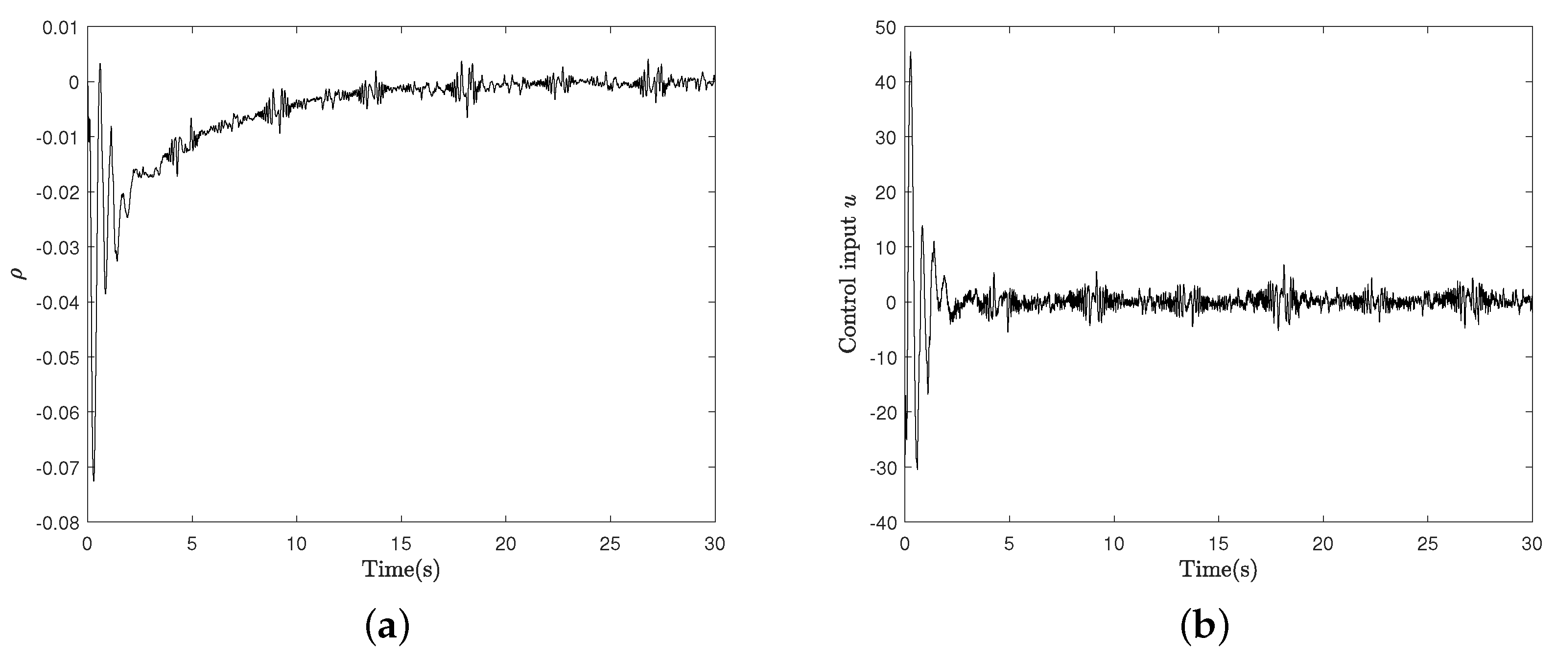
In Figure 4, the tracking control results and errors of the proposed approach and the previous controller [24] are compared. While the system output and tracking error of the previous controller [24] diverge, those of the proposed state-quantized controller converge. Therefore, the proposed adaptive state-quantized tracking approach can be used in the presence of input delay. Figure 5 shows the adaptive estimated parameters of the proposed state-quantized controller. Figure 6 displays the response of the input compensator and the control input of the proposed state-quantized controller. It is observed that all the closed-loop signals are bounded and the state-quantized tracking is successfully achieved in the presence of input delay.

5. Conclusions

This paper develops the adaptive state-quantized control strategy to compensate for the input delay of uncertain nonlinear lower-triangular systems with state quantization. The error surface using the auxiliary time-varying signal for compensating for the input delay is derived for the control design. A neural-network-based adaptive controller and its adaptive laws are constructed via quantized states while designing the input delay compensator using quantized states. In the proposed control scheme, the quantization errors and approximation errors are compensated via the adaptive technique and their boundedness is analyzed by establishing some technical lemmas. All involved signals are ensured to be bounded. The effectiveness of the proposed approach is demonstrated by the hydraulic servo dynamics. Compared with the existing quantized feedback control designs of nonlinear systems, the primary contribution of this paper is to provide the adaptive state-quantized control strategy in the presence of input delay. This paper provides a theoretical basis for the adaptive state-quantized control design in the presence of input delay. Thus, the proposed approach can be extended to various practical systems in the lower-triangular form such as aircraft wing rock models, jet engines, flight systems, biochemical processes, and flexible-joint robots reported in [1].

References

- Krstic, M.; Kanellakopoulos, I.; Kokotovic, P.V. Nonlinear and Adaptive Control Design; Wiley: New York, NY, USA, 1995. [Google Scholar]
- Swaroop, D.; Hedrick, J.K.; Yip, P.P.; Gerdes, J.C. Dynamic surface control for a class of nonlinear systems. IEEE Trans. Autom. Control 2000, 45, 1893–1899. [Google Scholar] [CrossRef] [Green Version]
- Farrell, J.A.; Polycarpou, M.; Sharma, M.; Dong, W. Command filtered backstepping. IEEE Trans. Autom. Control 2009, 54, 1391–1395. [Google Scholar] [CrossRef]
- Krstic, M. Input delay compensation for forward complete and strict-feedforward nonlinear systems. IEEE Trans. Autom. Control 2010, 55, 287–303. [Google Scholar] [CrossRef]
- Bekiaris-Liberis, N.; Krstic, M. Compensation of time-varying input and state delays for nonlinear systems. J. Dyn. Syst. Meas. Control 2012, 134, 011009. [Google Scholar] [CrossRef]
- Sharma, N.; Bhasin, S.; Wang, Q.; Dixon, W. Predictor-based control for an uncertain Euler-Lagrange system with input delay. Automatica 2011, 47, 2332–2342. [Google Scholar] [CrossRef]
- Kamalapurkar, R.; Fischer, N.; Obuz, S.; Dixon, W. Time-varying input and state delay compensation for uncertain nonlinear systems. IEEE Trans. Autom. Control 2016, 61, 834–839. [Google Scholar] [CrossRef]
- Obuz, S.; Klotz, J.R.; Kamalapurkar, R.; Dixon, W. Unknown time-varying input delay compensation for uncertain nonlinear systems. Automatica 2017, 76, 222–229. [Google Scholar] [CrossRef]
- Deng, W.; Yao, J.; Ma, D. Time-varying input delay compensation for nonlinear systems with additive disturbance: An output feedback approach. Int. J. Robust Nonlinear Control 2018, 28, 31–52. [Google Scholar] [CrossRef]
- Zuo, Z.; Lin, Z.; Ding, Z. Truncated predictor control of Lipschitz nonlinear systemswith time-varying input delay. IEEE Trans. Autom. Control 2016, 62, 5324–5330. [Google Scholar] [CrossRef]
- Khanesar, M.A.; Kaynak, O.; Yin, S.; Gao, H. Adaptive indirect fuzzy sliding mode controller for networked control systems subject to time-varying network-induced time delay. IEEE Trans. Fuzzy Syst. 2014, 23, 205–214. [Google Scholar] [CrossRef]
- Li, H.; Wang, L.; Du, H. BoulkrouneH. Adaptive fuzzy backstepping tracking control for strict-feedback systemswith input delay. IEEE Trans. Fuzzy Syst. 2017, 25, 642–652. [Google Scholar] [CrossRef]
- Wu, C.; Liu, J.; Jing, X.; Li, J.; Wu, L. Adaptive fuzzy control for nonlinear networked control systems. IEEE Trans. Syst. Man Cybern. 2017, 47, 2420–2430. [Google Scholar] [CrossRef]
- Li, D.P.; Liu, Y.J.; Tong, S.; Chen, C.P.; Li, D.J. Neural networks-based adaptive control for nonlinear state constrained systems with input delay. IEEE Trans. Cybern. 2018, 49, 1249–1258. [Google Scholar] [CrossRef]
- Ma, J.L.; Xu, S.; Li, Y.; Chu, Y.; Zhang, Z. Neural networks-based adaptive output feedback control for a class of uncertain nonlinear systems with input delay and disturbances. J. Frankl. Inst. 2018, 355, 5503–5519. [Google Scholar] [CrossRef]
- Niu, B.; Lu, L. Adaptive backstepping-based neural tracking control for MIMO nonlinear switched systems subject to input delays. IEEE Trans. Neural Netw. Learn. Syst. 2018, 29, 2638–2644. [Google Scholar] [CrossRef]
- Wang, H.; Liu, S.; Yang, X. Adaptive neural control for non-strict-feedback nonlinear systems with input delay. Inf. Sci. 2020, 514, 605–616. [Google Scholar] [CrossRef]
- Ma, J.; Xu, S.; Zhuang, G.; Wei, Y.; Zhang, Z. Adaptive neural network tracking control for uncertain nonlinear systems with input delay and saturation. Int. J. Robust Nonlinear Control 2020, 30, 2593–2610. [Google Scholar] [CrossRef]
- Wang, T.; Wu, J.; Wang, Y.; Ma, M. Adaptive fuzzy tracking control for a class of strict-feedback nonlinear systems with time-varying input delay and full state constraints. IEEE Trans. Fuzzy Syst. 2020, 28, 3432–3441. [Google Scholar] [CrossRef]
- Fu, M.; Xie, L. The sector bound approach to quantized feedback control. IEEE Trans. Autom. Control 2005, 50, 1698–1711. [Google Scholar]
- Montestruque, L.A.; Antsaklis, P.J. Static and dynamic quantization in model-based networked control systems. Int. J. Control 2007, 80, 87–101. [Google Scholar] [CrossRef]
- Zhou, J.; Wen, C.; Wang, W.; Yang, F. Adaptive backstepping control of nonlinear uncertain systems with quantized states. IEEE Trans. Autom. Control 2019, 64, 4756–4763. [Google Scholar] [CrossRef]
- Choi, Y.H.; Yoo, S.J. Quantized feedback adaptive command filtered backstepping control for a class of uncertain nonlinear strict-feedback systems. Nonlinear Dyn. 2020, 99, 2907–2918. [Google Scholar] [CrossRef]
- Choi, Y.H.; Yoo, S.J. Quantized-feedback-based adaptive event-triggered control of a class of uncertain nonlinear systems. Mathematics 2020, 8, 1603. [Google Scholar] [CrossRef]
- Choi, Y.H.; Yoo, S.J. Neural-networks-based adaptive quantized feedback tracking of uncertain nonlinear strict-feedback systems with unknown time delays. J. Frankl. Inst. 2020, 357, 10691–10715. [Google Scholar] [CrossRef]
- Brockett, R.W.; Liberzon, D. Quantized feedback stabilization of linear systems. IEEE Trans. Autom. Control 2000, 45, 1279–1289. [Google Scholar] [CrossRef] [Green Version]
- Park, J.; Sandberg, I.W. Universal approximation using radial-basis-function networks. Neural Comput. 1991, 3, 246–257. [Google Scholar] [CrossRef]
- Wang, C.; Hill, D.J.; Ge, S.S.; Chen, G.R. An ISS-modular approach for adaptive neural control of pure-feedback systems. Automatica 2006, 42, 625–635. [Google Scholar] [CrossRef]
- Kurdila, A.J.; Narcowich, F.J.; Ward, J.D. Persistency of excitation in identification using radial basis function approximants. SIAM J. Control Optim. 1995, 33, 625–642. [Google Scholar] [CrossRef]
- Hu, G.D.; Liu, M. The weighted logarithmic matrix norm and bounds of the matrix exponential. Linear Algebra Appl. 2000, 390, 145–154. [Google Scholar] [CrossRef] [Green Version]
- Liu, Y.; Zhu, Q. Adaptive neural network finite-time tracking control of full state constrained pure feedback stochastic nonlinear systems. J. Frankl. Inst. 2020, 357, 6738–6759. [Google Scholar] [CrossRef]
- Gao, T.; Liu, Y.J.; Li, D.; Tong, S.; Li, T. Adaptive neural control using tangent time-varying BLFs for a class of uncertain stochastic nonlinear systems with full state constraints. IEEE Trans. Cybern. 2021, 51, 1943–1953. [Google Scholar] [CrossRef] [PubMed]
- Zhu, Q.; Liu, Y.; Wen, G. Adaptive neural network control for time-varying state constrained nonlinear stochastic systems with input saturation. Inf. Sci. 2020, 527, 191–209. [Google Scholar] [CrossRef]
- Sun, Y.M.; Chen, B.; Liu, C.; Wang, H.H.; Zhou, S.W. Adaptive neural control for a class of stochastic nonlinear systems by backstepping approach. Inf. Sci. 2016, 369, 748–764. [Google Scholar] [CrossRef]
- Na, J.; Li, Y.; Huang, Y.; Gao, G.; Chen, Q. Output feedback control of uncertain hydraulic servo systems. IEEE Trans. Ind. Electron. 2020, 67, 490–500. [Google Scholar] [CrossRef]
Figure 1.
Comparison of tracking results and errors for Example 1: (a) y and of the proposed control system; (b) y and of the control system presented in [24]; (c) of the proposed control system; and (d) of the control system presented in [24].
Figure 2.
Estimation results of the proposed control system for Example 1 (a) , ; and (b) , .
Figure 3.
Input delay compensator and control input of the proposed control system for Example 1: (a) ; and (b) u.
Figure 4.
Comparison of tracking results and errors for Example 2: (a) y and yr of the proposed control system; (b) y and yr of the control system presented in [24]; (c) s1 of the proposed control system; and (d) s1 of the control system presented in [24].
Figure 5.
Estimation results of the proposed control system for Example 2: (a) , ; and (b) , .
Figure 6.
Input delay compensator and control input of the proposed control system for Example 2: (a) ; and (b) u.
Publisher’s Note: MDPI stays neutral with regard to jurisdictional claims in published maps and institutional affiliations. |
© 2021 by the author. Licensee MDPI, Basel, Switzerland. This article is an open access article distributed under the terms and conditions of the Creative Commons Attribution (CC BY) license (https://creativecommons.org/licenses/by/4.0/).
Share and Cite
MDPI and ACS Style
Yoo, S.J. Adaptive State-Quantized Control of Uncertain Lower-Triangular Nonlinear Systems with Input Delay. Mathematics 2021, 9, 763. https://doi.org/10.3390/math9070763
AMA Style
Yoo SJ. Adaptive State-Quantized Control of Uncertain Lower-Triangular Nonlinear Systems with Input Delay. Mathematics. 2021; 9(7):763. https://doi.org/10.3390/math9070763
Chicago/Turabian StyleYoo, Sung Jin. 2021. "Adaptive State-Quantized Control of Uncertain Lower-Triangular Nonlinear Systems with Input Delay" Mathematics 9, no. 7: 763. https://doi.org/10.3390/math9070763
Note that from the first issue of 2016, this journal uses article numbers instead of page numbers. See further details here.