A Continuous Review Production-Inventory System with a Variable Preparation Time in a Fuzzy Random Environment

Abstract

With the increase in the varieties products and the increasing uncertainty about product demand, the production preparation time is a significant factor in addressing these issues. The trade-off between the reduction of the production preparation time and the associated cost remains a critical decision. With this backdrop, this study presents a continuous review production-inventory model with a variable production preparation time and a time-dependent setup cost. The demand during the preparation time is captured through a min-max distribution-free approach. In a stochastic framework, the order quantity, reorder point, and setup time are optimized by minimizing the expected cost considering the time-value effect. Further, a fuzzy model is formulated to tackle the imprecise nature of the production setup time and demand. Two algorithms are developed using an analytical approach to obtain the optimal solution. A numerical illustration is given to present the key insights of the model for effective inventory management. It is observed that order quantity and total cost are more sensitive at the lower side of the optimal setup time rather than at the higher side. The discount rate is also found to be a sensitive factor while minimizing the total expected cost.

1. Introduction

With globalization, organizations must cater to ever-changing consumer demand by offering a wide variety of products. An inventory system is studied to understand the movement of goods through the different phases of a manufacturing cycle in a systematic manner. The economic order quantity (EOQ) and economic production quantity (EPQ) models have been extensively used since their development and have been extended over time to incorporate more realistic aspects, as well as to relax the basic assumptions. Between the continuous review and the periodic review, the continuous review has received more attention due to its mathematical approach and ability to handle diverse problems.

In this study, we focus on the EPQ model in dealing with the preparation time and related aspects. In the past decade, several authors have developed various EPQ models with different factors under the stochastic framework [1,2,3,4,5]. Sarker and Coates [6] considered deterministic demand and the production rate with production lead-time to be finite range random variables. Sarkar et al. [7] extended the model of Moon and Choi [8] to reduce the setup cost and improve its quality in a continuous review inventory model by applying a distribution-free approach. Panda et al. [1] and Sarkar and Moon [2] formulated a single period production-inventory model assuming a deterministic production rate and random demand when scheduling in the stochastic environment. An EPQ model with an imperfect production process, inflation, and stochastic demand was developed by Krishnamoorthi and Panayappan [9]. Mukhopadhyay and Goswami [10] developed an EPQ model for imperfect production using partial fractions to reduce the total production cost. Kumar and Goswami [5] also developed a stochastic model for the continuous review production-inventory model considering the min-max distribution-free approach. Choudri et al. [11] considered the effect of inflation and the time value of money to analyze an inventory control system for deteriorating products with constant demand. The imperfect EPQ model introduced by Kundu et al. [12] has the advantage of time-sensitive production and demand to show the effects of defect rates on production costs. Lin [13] developed an optimal production-inventory policy for a stochastic EPQ inventory system with imperfect production processes and rework processes. Recently, Singer and Khmelnitsky [14] developed a production-inventory model with price-sensitive demand as a Wiener stochastic process where a manufacturer decides both the operational policy and the pricing policy with an optimal price for a product.

In general, the preparation time in a production-inventory model is assumed to be zero. However, there is always a time gap between the decision to start the production process and the actual start of production, which is termed the “production preparation time”. The production preparation time includes several mutually independent components such as: (i) making preparation decisions; (ii) collecting raw materials; (iii) screening raw materials; and (iv) servicing machines. The setup cost and production cost in a production-inventory model depend significantly on the production preparation time [15]. Estimating the production preparation time is difficult due to its imprecise nature. To tackle this issue, researchers and practitioners have used fuzzy models [16]. Bag et al. [17] developed an imperfect production system under flexibility and reliability using fuzzy random demand. Soni and Shah [18] developed an EPQ model with both imprecise demand and production preparation time as fuzzy variables along with shortages and full backlogs. Jana et al. [19] considered an inventory model including items that deteriorate over a random planning period under conditions of inflation and the time value of money. Mondal et al. [20] analyzed a production-inventory model in the presence of inflation and the time value of money in a fuzzy rough environment. Soni et al. [21] considered the effects of lost sales and quality improvements in an imperfect production system in a fuzzy environment. Bhuiya et al. [22] extended Sana and Goyal’s model [23] by calculating the optimal order quantity, reorder point, and lead-time simultaneously in a random framework, as well as considering uncertain demand to be a fuzzy random variable. Dey [24] developed an integrated single-vendor/single-buyer imperfect production-inventory model in which fuzziness and randomness simultaneously appear in a mixed environment. Fu et al. [25] developed a production-inventory model to determine the optimal decision in a single-vendor/single-buyer supply chain system by considering imperfect quality, the learning effect, and triangular fuzzy demand. In [26], for the first time, reliable and unreliable sellers were considered in a coordination supply chain model. The profitability of the supply chain was determined using a variable setup cost, order quantity, and service level. This model is seen as more realistic by considering lead-time demand to be stochastic, where the distribution is unknown. The model also uses a distribution-free approach to solve the problem. Hemalatha and Annadurai [27] extended the work of Priyan and Uthayakumar [28] by considering the parameters as the triangular fuzzy number for an integrated production-distribution inventory system with deteriorating products. Sarkar and Mahapatra [29] extended the work of Annadurai and Uthayakumar [30] by developing a periodic review inventory model with a fuzzy demand pattern. They minimized the expected total annual cost by simultaneously optimizing the cycle length, reorder point, and lead-time for the whole system based on fuzzy demand. Recently, Mahapatra et al. [31] developed a fuzzy EOQ model to analyze the impact of learning to reduce fuzziness within a finite time horizon, as well as to consider the effect of promoting deteriorating items.

Most research on inventory models does not consider the effect of inflation and the time value of money in global economics. This is somewhat away from real scenarios, since the basis of their uniqueness is dependent on when the model is used, which is highly connected to the stock return. In the case of investment and forecasting, the time value of money should be critically accounted for. The inflationary effect and influence of the time value of money are significant for improving decision-making and remaining financially sound in today’s highly competitive market. Moon and Yun [32] developed a discounted cash flow approach by considering the time value of money and a random planning horizon variable. Shah [33] analyzed an inventory model by accounting for a constant deterioration unit cost and the time value of money when payments are delayed considerably. Dey et al. [34] considered an inventory model of the deterioration of items under the time value of money and inflation rates. Hou et al. [35] formulated an inventory model based on the inflation rate and time value of money for a certain period and a planning scale, considering deteriorating products with partial back orders. Hung [36] developed a continuous inventory model using the time value of money in which preparation time demand follows a normal distribution. Shah and Vaghela [37] developed an inventory model with effort-dependent and time-dependent demand by considering the time value of money and inflation effects. Pérez et al. [38] analyzed an EPQ inventory model with pre- and post-deterioration discounts on the selling price, considering the time value of money and partial back order shortages.

Motivation and Objective

Based on the above-mentioned literature, it can be found that studies on variable preparation time are rare. The same can be easily understood from the comparison of the previous literature as presented in

Table 1. Comparison of the contributions of different authors.

Author(s)	Model	Distribution	Variable	Order	Time	Fuzzy	Partial	Variable
	Structures	Free Approach	Preparation Time	Quantity	Value Effect	Random Demand	Backorder Cost	Reorder Point
Dey et al. [34]	EOQ			√	√		√
Bag et al. [17]	EPQ					√
Sarkar and Moon [2]	EPQ			√	√
Soni and Shah [18]	EPQ		√	√
Wang [39]	EOQ	√		√		√	√
Hou et al. [35]	EOQ			√	√		√
Mondal et al. [20]	EPQ				√
Mukhopadhyay and Goswami [10]	EPQ	√
Wee et al. [4]	EPQ			√			√
Kumar and Goswami [5]	EPQ	√		√		√		√
Soni and Patel [40]	SCM			√		√	√	√
Choudri et al. [11]	EPQ			√	√
Hung [36]	EOQ		√	√	√
Sarkar and Mahapatra [29]	EOQ	√		√		√	√	√
Soni et al. [41]	EOQ			√		√	√	√
Soni et al. [21]	EPQ			√
Shah and Vaghela [37]	EPQ			√	√
Tayyab et al. [42]	MPS			√		√
Mahapatra et al. [31]	EOQ			√		√	√
Kundu et al. [12]	EPQ			√		√
Sarkar and Chung [43]	SCM			√			√
Mishra et al. [44]	EPQ			√			√
Singer and Khmelnitsky [14]	EPQ			√			√
This study	EPQ	√	√	√	√	√	√	√

. Apart from the particular issue of variable production time, the model complexity increases as we include other practical aspects such as stochastic demand, imprecise attributes, and time value features. Therefore, the reduction of the total inventory cost considering the above-mentioned aspects is a real challenge that motivates us to take up the problem. In this regard, an effort is made to address to optimize variable production time in a stochastic environment with imprecise attributes by minimizing the total expected inventory cost.

Considering all the features, the contribution and novelty of the present study are as follows:

• This study extends the work of [5] by proposing a production-inventory model that allows for a stochastic environment with a variable production setup time and partial back orders considering the time value of money. They focused on how to use the historical data when the demand distribution is not known. It is also a fact that the adequate demand information does not come with ease. However, through historical data, the mean and variance of the distribution function of demand can be calculated. They optimized the inventory strategy against the most unfavorable distribution of demand by treating it as an FRV and extending the MMDFP for said FRV. They considered the production setup time as a parameter and performed sensitivity analysis, whereas the production setup time is a decision variable in this study where the opportunity for the crashing of sub-tasks is available.
• In this investigation, an imperfect EPQ model in a fuzzy environment is developed, which offers more practical scenarios, as well as accounts for the imprecise nature of demand and the production setup time.
• The model considers the fuzzy demand rate and production preparation time with known distribution functions, where the production cost and setup cost are taken as a function of the preparation time.
• The shortage cost and holding cost are considered to be a proportion of the production cost.

The rest of the paper is organized as follows. Section 2.1 presents all the notations and necessary assumptions. Section 2.2 describes the stochastic inventory model, and Section 2.3 describes the fuzzy stochastic inventory model. The results of the numerical experiments are presented in Section 3 using input data along with the sensitivity analyses of the key parameters. Finally, Section 4 concludes. Compliance with ethical standards and a list of the abbreviations used in the model are also given.

2. Mathematical Model

This section starts with the basic assumptions and notations of the model.

2.1. Assumptions and Notations

The following assumptions and notations are used throughout the paper to develop this model.

Assumptions:

• The setup cost depends on the setup time as follows: $A\left(L\right)=a_0+a_1{L}^{-\gamma }$, where $a_0\mathrm{and}{a}_1$ are non-negative real numbers and $\gamma >0$. If the setup is planned in advance, some components of the setup cost (e.g., labor, wages) may be reduced (Soni and Shah [18]).
• The effect of inflation and the time value of money is considered [45,46].
• The setup time L has n mutually independent components such as collecting raw materials, screening raw materials, and servicing machines. There are varying reduction costs for each component to curtail the setup time. The r$\mathrm{th}$ component has a minimum duration $a_r$ and normal duration $b_r$, as well as a reduction cost per unit time $c_r$. Furthermore, it is assumed that $c_1\le c_2\le \dots \le c_n$.
• Let $L_0={\sum }_{r=1}^n{b}_r$ and $L_p$ be the setup time with the components $1,2,\dots ,p$ reduced to their minimum duration; then, $L_p$ can be expressed as $L_p={\sum }_{r=1}^n{b}_r-{\sum }_{r=1}^p(b_r-a_r),p=1,2,\dots ,n$. The per cycle setup time reduction cost $C\left(L\right)$ is as follows:

  $$\begin{array}{ccc}\hfill C\left(L\right)& =& c_p(L_p-L)+\sum _{r=1}^{p-1}{c}_r(b_r-a_r)\hfill \\ \hfill \mathrm{and}C\left(L_0\right)& =& 0,\mathrm{for}\mathrm{all}L\in [L_p,L_{p-1}]\hfill \end{array}$$

  (1)
• During the i$\mathrm{th}$ unit of time, the demand rate $X_i$ is random and independent of previous and forthcoming epochs (i.e., $X_i,i=1,2,\dots$ are independent random variables with identical mean d and variance ${\sigma }^2$).
• Demand during the preparation time, X, is a convolution of the demand rate $X_i$ and the preparation time L (Kim et al. [47]). Hence, $E\left[X\right]={\sum }_{i=1}^{L}E\left[X_i\right]=dL$ and $var\left[X\right]={\sum }_{i=1}^{L}var\left[X_i\right]=L{\sigma }^2$. For notional convenience, $d_L=dL$ and ${\sigma }_L^2={\sigma }^{2}L$.
• Preparation time demand, a random variable, follows an unknown distribution function with finite mean $dL$ and variance ${\sigma }^{2}L$. The min-max distribution-free procedure finds the worst possible distribution and then minimizes the total expected cost. The expected shortage is calculated based on the work of Kumar and Goswami [5,48]):

  $$\begin{array}{c}\hfill E{\left[X-R\right]}^{+}=\frac{\sqrt{{\sigma }^{2}L+{(R-d_L)}^2}-(R-d_L)}{2}\end{array}$$

  (2)
• The production preparation time is the time between the decision to start production and actual commencement of production.
• Shortages are allowed and backlogged partially.
• The time horizon is infinite (Kumar and Goswami [5]).

Notations:

Model parameters and variables are presented in

Table 2. Model parameters and decision variables.

Parameters
D	Expected demand per year (units)
P	Production rate per unit time ($P>D$)
$A\left(L\right)$	Setup cost per cycle with preparation time
$d_L$	Mean demand during the preparation time
$\sigma$	Standard deviation of demand during the preparation time
$\tau$	Proportion of back orders during the stockout period
h	Inventory holding cost ($/unit)
s	Inventory shortage cost ($/unit)
$\pi$	Marginal profit ($/unit)
$\theta$	Interest rate per year, compounded continuously
$L_p$	Length of the preparation time for component p
	where $p=1,2,\dots ,n$
$a_r$	Minimum preparation time for component r (days)
$b_r$	Normal preparation time for component r (days)
$c_r$	Crashing cost per unit time for component r
$E(.)$	Mathematical expectation of $(.)$
$x^{+}$	$max\{x,0\}$
X	Random demand during the preparation time, which lies within
	the finite interval with mean $d_L=dL$ and variance ${\sigma }_L^2={\sigma }^{2}L$
$X_i$	Random demand rate, which varies within the finite interval,
	i.e., $X_i\left(\omega \right)=x\in [x_{min},x_{max}]$; the mean and variance of $X_i$ are
	$d_L$ and ${\sigma }_L^2$, respectively
F	Family of distribution functions with mean $d_L$ and variance ${\sigma }_L^2$
$\mathcal{F}$	Class of cumulative distribution function with
	mean $d_L$ and variance ${\sigma }_L^2$
Decision variables
Q	Order quantity per cycle
R	Reorder point
L	Preparation time for replenishment

.

2.2. Stochastic Inventory Model

In this section, a continuous review production-inventory model is considered in which items are produced internally and concurrently to meet customers’ demand. The inventory level pattern can be described as follows: When the inventory level falls to R units, management decides to start the production of amount Q. Owing to the preparation time of the production process, the actual production rate of $(P-D)$ is started after the L unit of time, which continues to time $t_p=\frac{Q}{P}$. Thereafter, the inventory level is reduced at the rate D due to demand only. The length of one cycle is $\frac{Q}{D}$. Figure 1 illustrates the model.

Therefore, the total expected cost is given by $TEC=\mathrm{Setup}\mathrm{cost}+\mathrm{Holding}\mathrm{cost}+\mathrm{Shortage}\mathrm{cost}+\mathrm{Lost}\mathrm{sales}\mathrm{cost}+\mathrm{Setup}\mathrm{time}\mathrm{reduction}\mathrm{cost}.$

In this study, the production-inventory model takes into account the time value of money. When production starts, the expected on-hand inventory level is $R-d_L+(1-\tau )E{[X-R]}^{+}$; then, at the end of the production process, the expected maximum inventory level is $(P-D)\frac{Q}{P}+R-d_L+(1-\tau )E{[X-R]}^{+}$. Since the value of an inventory item is no longer constant, the holding cost becomes a function of the inflation used to determine the value of the ending inventory.

Hence, the expected holding cost for the inventory system with the effect of inflation for the first cycle is:

$$\begin{array}{ccc}& & h{\int }_0^{Q/P}\left\{R-d_L+\left(1-\tau \right)E{\left[X-R\right]}^{+}+\left(P-D\right)t\right\}{e}^{-\theta t}dt\hfill \\ & +& h{\int }_{Q/P}^{Q/D}\left\{\left(P-D\right)Q/P+R-d_L+\left(1-\tau \right)E{\left[X-R\right]}^{+}-D\left(t-\frac{Q}{P}\right)\right\}{e}^{-\theta t}dt\hfill \\ & =& {\displaystyle \frac{h\left(R-d_L+\left(1-\tau \right)E{\left[X-R\right]}^{+}\right)\left(1-e^{-\theta Q/D}\right)}{\theta }}+{\displaystyle \frac{hP\left(1-e^{-\theta Q/P}\right)}{{\theta }^2}}\hfill \\ & -& {\displaystyle \frac{hD\left(1-e^{-\theta Q/D}\right)}{{\theta }^2}}\hfill \end{array}$$

(3)

The discounted cash flow approach is adopted under which cash outflows occur for the setup cost, shortage cost, lost sales cost, and setup time reduction cost at the beginning of each cycle. The basics of the discounted cash flow can be found in the works of Moon and Yun [32] and Mondal et al. [20]. Therefore, the total relevant expected cost for the first cycle is given by:

$$\begin{array}{ccc}\hfill TREC(Q,R,L)& =& A\left(L\right)+h\left(R-d_L+\left(1-\tau \right)E{\left[X-R\right]}^{+}\right){\displaystyle \frac{\left(1-e^{-\theta Q/D}\right)}{\theta }}\hfill \\ & +& {\displaystyle \frac{hP\left(1-e^{-\theta Q/P}\right)}{{\theta }^2}}-{\displaystyle \frac{hD\left(1-e^{-\theta Q/D}\right)}{{\theta }^2}}\hfill \\ & +& E{\left[X-R\right]}^{+}\left[s+\pi (1-\tau )\right]+C\left(L\right)\hfill \end{array}$$

(4)

According to Silver et al. [49], the present value of the expected total relevant cost over the infinite time horizon, $PVC(Q,R,L)$, is given by:

$$\begin{array}{c}\hfill PVC(Q,R,L)=\frac{1}{1-e^{-\theta Q/D}}TREC(Q,R,L)\end{array}$$

(5)

for $0<Q,R<\infty$ and $L_n\le L\le L_0$.

In many real-life situations, information on preparation time demand is limited. If the probability distribution of demand during preparation time X is unknown or many distribution functions have the same mean and variance, then the exact value of $E{(X-R)}^{+}$ cannot be obtained. Hence, the optimal value of $PVC(Q,R,L)$ cannot be found. Therefore, the min-max distribution-free approach (see Appendix B) is applied to solve the problem of the following form:

$$\begin{array}{c}\hfill {\mathrm{Min}}_{Q>0}{\mathrm{Max}}_{\mathbf{F}\in \mathcal{F}}PVC(Q,R,L)\end{array}$$

This task was greatly simplified by Scarf [50], who proved the following Lemma 1.

Lemma 1.

For any $\mathit{F}\in \mathcal{F}$,

$$E{\left[X-R\right]}^{+}\le \frac{\sqrt{{\sigma }^{2}L+{(R-d_L)}^2}-(R-d_L)}{2}$$

(6)

Moreover, for every R, there exists a distribution $F^{\ast }\in \mathcal{F}$, where the upper bound is tight.

Thus,

$$PVC(Q,R,L)\le {\displaystyle \frac{f(R,L)}{1-e^{-\theta Q/D}}}+g(R,L)+{\displaystyle \frac{hP}{{\theta }^2}}{\displaystyle \frac{1-e^{-\theta Q/P}}{1-e^{-\theta Q/D}}}$$

(7)

where

$$\begin{array}{ccc}\hfill f(R,L)& =& A\left(L\right)+C\left(L\right)+\left[s+\pi (1-\tau )\right]U(R,L)\hfill \\ \hfill g(R,L)& =& {\displaystyle \frac{h[R-d_L+(1-\tau )U(R,L)]}{\theta }}-{\displaystyle \frac{hD}{{\theta }^2}}\hfill \\ \hfill U(R,L)& =& {\displaystyle \frac{\sqrt{{\sigma }^{2}L+{(R-d_L)}^2}-(R-d_L)}{2}}\hfill \end{array}$$

To solve Equation (7), taking the first-order partial derivative of $PVC(Q,R,L)$ with respect to Q and keeping R fixed, we obtain:

$${\displaystyle \frac{\partial PVC(Q,R,L)}{\partial Q}}={\displaystyle \frac{F\left(Q\right)}{D\theta e^{\theta Q/D}{\left(1-e^{-\theta Q/D}\right)}^2}}$$

(8)

where $F\left(Q\right)=h(P-D)e^{-\theta Q/P}(1+e^{\theta Q/D})-{\theta }^{2}f(R,L)$

Differentiating $F\left(Q\right)$ with respect to Q, we obtain:

$${\displaystyle \frac{dF}{dQ}}={\displaystyle \frac{h\theta (P-D)e^{-\theta Q/P}\left[(P-D)e^{\theta Q/D}-D\right]}{PD}}>0$$

Thus, $F\left(Q\right)$ is a strictly increasing function of Q. Moreover, $F\left(0\right)=2h(P-D)-{\theta }^{2}f(R,L)$ and ${\displaystyle \underset{Q\to \infty }{lim}F\left(Q\right)=+\infty }$. Hence, if $F\left(0\right)<0$, then, according to the intermediate value theorem (Olsen [51]), a unique value of Q exists (e.g., $Q^{\ast }$) such that $F\left(Q^{\ast }\right)=0$. Hence,

$$h(P-D)e^{-\theta Q^{\ast }/P}(1+e^{\theta Q^{\ast }/D})={\theta }^{2}f(R,L)\Rightarrow e^{-\theta Q^{\ast }/P}+e^{\theta Q^{\ast }(P-D)/PD}=\frac{{\theta }^{2}f(R,L)}{h(P-D)}$$

(9)

Furthermore,

$$\begin{array}{c}\hfill {\left[{\displaystyle \frac{{\partial }^{2}PVC(Q,R,L)}{\partial Q^2}}\right]}_{Q=Q^{\ast }}={\displaystyle \frac{h(P-D)e^{-\theta Q/P}\left[(P-D)e^{\theta Q/D}-D\right]}{P{D}^2{e}^{\theta Q/D}{\left(1-e^{-\theta Q/D}\right)}^2}}>0\end{array}$$

Therefore, $PVC(Q,R,L)$ is a convex function in Q because the second-order sufficient conditions are satisfied. Again, taking the first- and second-order partial derivatives of $PVC(Q,R,L)$ with respect to R and keeping Q fixed, we obtain:

$${\displaystyle \frac{\partial PVC(Q,R,L)}{\partial R}}=\left[{\displaystyle \frac{R-d_L}{\sqrt{{\sigma }^{2}L+{(R-d_L)}^2}}}-1\right]\left[{\displaystyle \frac{(s+\pi (1-\tau \left)\right)}{2(1-e^{-\theta Q/D})}}+\frac{h(1-\tau )}{2\theta }\right]+\frac{h}{\theta }$$

(10)

$${\displaystyle \frac{{\partial }^{2}PVC(Q,R,L)}{\partial R^2}}=\left[{\displaystyle \frac{{\sigma }^{2}L}{{\{{\sigma }^{2}L+{(R-d_L)}^2\}}^{\frac{3}{2}}}}\right]\left[{\displaystyle \frac{(s+\pi (1-\tau \left)\right)}{2(1-e^{-\theta Q/D})}}+\frac{h(1-\tau )}{2\theta }\right]>0$$

(11)

It can be verified that $PVC(Q,R,L)$ is a convex function in $R\in (0,\infty )$ by calculating the second-order sufficient conditions.

Again, when Equation (10) is equal to zero, we obtain:

$${\displaystyle \frac{R-d_L}{\sqrt{{\sigma }^{2}L+{(R-d_L)}^2}}}=\lambda \Rightarrow R=d_L\pm {\displaystyle \frac{\lambda \sigma \sqrt{L}}{\sqrt{1-{\lambda }^2}}}$$

(12)

$$\lambda ={\displaystyle \frac{\left[\theta \{s+\pi (1-\tau )\}\right]-h(1+\tau )[1-e^{-\frac{\theta Q}{D}}]}{\left[\theta \{s+\pi (1-\tau )\}\right]+h(1-\tau )[1-e^{-\frac{\theta Q}{D}}]}}$$

Therefore, from Equation (7), we obtain:

$$PVC(Q^{\ast },R^{\ast },L^{\ast })={\displaystyle \frac{f(R^{\ast },L^{\ast })}{1-e^{-\theta Q^{\ast }/D}}}+g(R^{\ast },L^{\ast })+{\displaystyle \frac{hP}{{\theta }^2}}{\displaystyle \frac{1-e^{-\theta Q^{\ast }/P}}{1-e^{-\theta Q^{\ast }/D}}}$$

(13)

Using the following algorithm, the optimal solution of $(Q,R,L)$ is obtained from Equations (9), (12), and (13). Moreover, the computational procedure for obtaining the optimum solution of $(Q,R,L)$ is explained, which is denoted by $(Q^{\ast },R^{\ast },L^{\ast })$. An improved Algorithm 1 is developed and presented below.

Algorithm 1: Steps for finding the optimal solution for the stochastic model.

Step 1 Input all the parameters.

Step 2 Perform Step 3 to Step 6 for each L from 63 to 21 in reverse order.

Step 3 Calculate $C\left(L\right)$ by crashing components $(p=1,2,\dots ,4)$ from the lowest unit cost to the highest unit cost to have a preparation time of L. For example, $C\left(L\right|63)=0$; $C\left(L\right|62)=0.04$, and so on.

Step 4 Calculate the $A\left(L\right)$ values based on the equation $A\left(L\right)=a_0+a_1{L}^{-\gamma }$, as mentioned in Assumption 1.

Step 5 Find the optimal values of $Q_L^{\ast }$ and $R_L^{\ast }$ and the $PVC(Q,R,L)$ value for the parametric value of L, as mentioned in Step 2, by minimizing $PVC(Q,R,L)$, as developed in Equation (13).

Step 6 Calculate the $SS$ values based on R and L.

Step 7 Select the ($Q^{\ast }$, $R^{\ast }$, $L^{\ast }$) corresponding to the lowest value of $PVC(Q,R,L)$.

Step 8 Present all the required outputs.

2.3. Fuzzy Stochastic Inventory Model

Contrary to the crisp inventory model in Section 2.2, a fuzzy stochastic framework takes into account the variability in certain demand parameters. The mathematical FRV (fuzzy random variable) model described in Section 1 accounts for the linguistic imprecision and mathematical uncertainty that occur because of disturbances in inventory frameworks. However, many researchers consider fuzzy demand [29,41,42], using the distribution-free approach. The computation of demand must first account for a plethora of factors such as the collection of data, their proper encoding, presaging the ensuing market conditions, and documentation, which are extremely erratic and variable. Thus, the estimation of demand by management must incorporate a fuzzy model that expresses that demand in the i$\mathrm{th}$ unit of time is “about $\widetilde{x_i}$,” which varies randomly in the interval $[x_{min},x_{max}]$. This assemblage can be mathematically expressed in terms of the FRV. Let $(\mathsf{\Omega },\mathcal{B},Pr)$ be a probability space in which $\mathsf{\Omega }$ is a sample space, $\mathcal{B}$ is the $\sigma$-algebra of the subsets $\mathsf{\Omega }$, and $Pr$ is a probability measure. Fuzzy random demand $\tilde{X}$, corresponding to the real-valued random demand $X_i$ at the $i\mathrm{th}$ unit of time, is a mapping from $\mathsf{\Omega }$ to a collection of fuzzy variables ${\mathcal{F}}_{\mathcal{R}}$ [52,53]. Without loss of generality, it is assumed that all the observed values of FRV ${\tilde{X}}_i$ are triangular fuzzy numbers; that is, for each $\omega \in \mathsf{\Omega }$, ${\tilde{X}}_i\left(\omega \right)=(X_i\left(\omega \right)-{\Delta }_i,X_i\left(\omega \right),X_i\left(\omega \right)+{\Delta }_i^{\prime })$ with the membership function ${\mu }_{{\tilde{X}}_i}$ as:

$${\mu }_{{\tilde{X}}_i}\left(\omega \right)=\left\{\begin{array}{c}{\displaystyle \frac{\omega -x_i+{\Delta }_i}{{\Delta }_i}},\mathrm{if}{x}_i-{\Delta }_i\le \omega \le x_i\hfill \\ {\displaystyle \frac{x_i+{\Delta }_i^{\prime }-\omega }{{\Delta }_i^{\prime }}},\mathrm{if}{x}_i\le \omega \le x_i+{\Delta }_i^{\prime }\hfill \\ 0,\mathrm{otherwise}.\hfill \end{array}\right.$$

If the length of the preparation time is L, then demand during the setup time is an L-fold convolution of the distribution ${\tilde{X}}_i$, which is represented by:

$$\tilde{X}={\tilde{X}}_1\oplus {\tilde{X}}_2\oplus \cdots \oplus {\tilde{X}}_L$$

where ${\tilde{X}}_i$ is the FRV, representing demand at the $i\mathrm{th}$ unit of time. Hence, $\tilde{X}=(X-{\delta }_1,X,X+{\delta }_2)$, where $X={\sum }_1^L{X}_i$, ${\delta }_1={\sum }_1^L{\Delta }_i$, and ${\delta }_2={\sum }_1^L{\Delta }_i^{\prime }$. Since the demand rate is fuzzy random in nature, the cycle time $Q/D$ is also fuzzy random in nature.

Therefore, the current value of the expected total relevant cost over an infinite time horizon in the fuzzy sense, $\widetilde{PVC}(Q,R,L)$, is given by:

$$\widetilde{FPVC}(Q,R,L)={\displaystyle \frac{\tilde{M}(R,L)}{1-e^{-\theta Q/\tilde{D}}}}+\tilde{N}(R,L)+{\displaystyle \frac{hP}{{\theta }^2}}{\displaystyle \frac{1-e^{-\theta Q/P}}{1-e^{-\theta Q/\tilde{D}}}}$$

(14)

where

$\tilde{M}(R,L)=A\left(L\right)+C\left(L\right)+\left[s+\pi (1-\tau )\right]E{[\tilde{X}-R]}^{+}$,

$\tilde{N}(R,L)={\displaystyle \frac{h[R-{\tilde{d}}_L+(1-\tau )E{[\tilde{X}-R]}^{+}]}{\theta }}-{\displaystyle \frac{h\tilde{D}}{{\theta }^2}}$

From the decomposition theorem, the objective function $\widetilde{FPVC}(Q,R,L)$ is represented by:

$$\widetilde{FPVC}(Q,R,L)=\bigcup _{\alpha \in \left[0,1\right]}\left[FPV{C}_{\alpha }^{-},FPV{C}_{\alpha }^{+};\alpha \right]$$

(15)

Employing the signed distance method (Yao and Wu [54]) (see Appendix C) to defuzzify the fuzzy annual cost $\widetilde{FPVC}(Q,R,L)$, we obtain:

$$\begin{array}{c}\hfill \widetilde{FPVC}(Q,R,L)={\displaystyle \frac{1}{2}}\underset{0}{\overset{1}{\int }}\left[FPV{C}_{\alpha }^{-}+FPV{C}_{\alpha }^{+}\right]d\alpha \end{array}$$

(16)

2.4. Calculation of the $\alpha$-Cut of $E{[\tilde{X}-R]}^{+}$

For a fixed reorder point R, the expressions of $E{({[\tilde{X}-R]}^{+})}_{\alpha }^{+}$ and $E{({[\tilde{X}-R]}^{+})}_{\alpha }^{-}$, which correspond to the random variables ${({[\tilde{X}-R]}^{+})}_{\alpha }^{+}$ and ${({[\tilde{X}-R]}^{+})}_{\alpha }^{-}$, respectively, can be estimated using the relationship between the value of x of fuzzy demand during the preparation time $\tilde{X}\left(x\right)$ and reorder point R. For every $x\in \mathsf{\Omega },(\tilde{X}-R)\left(x\right)=(x-R-{\delta }_1,x-R,x-R+{\delta }_2)$. Thus, for fixed values of $R, {\delta }_1$, and ${\delta }_2$, the expressions of ${({[\tilde{X}-R]}^{+})}_{\alpha }^{+}$ and ${({[\tilde{X}-R]}^{+})}_{\alpha }^{-}$ can be determined based on the following four situations, where demand x falls into the intervals $[R+{\delta }_1,\infty ),[R,R+{\delta }_1],$$[R-{\delta }_2,R],\mathrm{and}(-\infty ,R-{\delta }_2]$. To simplify the notation, let us denote $\tilde{Y}={[\tilde{X}-R]}^{+}$. For each situation, the $\alpha$-cut of $\tilde{Y}$ and correspondingly the $\alpha$-cut of the expectation $E[\tilde{Y}]$ are found.

Situation 1: $x\in [R+{\delta }_1,\infty )$, i.e., $x-R-{\delta }_1\ge 0$. Figure 2 shows the fuzzy shortage quantity $\tilde{Y}$.

The membership function ${\mu }_{\tilde{Y}}$ of $\tilde{Y}$ is:

$${\mu }_{\tilde{Y}}\left(y\right)=\left\{\begin{array}{cc}{\displaystyle \frac{y-(x-R-{\delta }_1)}{{\delta }_1}},\hfill & x-R-{\delta }_1\le y\le x-R\hfill \\ {\displaystyle \frac{(x-R+{\delta }_2)-y}{{\delta }_2}},\hfill & x-R\le y\le x-R+{\delta }_2\hfill \\ 0,\hfill & \mathrm{otherwise}.\hfill \end{array}\right.$$

where $\alpha$-cut $[{\tilde{Y}}_{\alpha }^{-},{\tilde{Y}}_{\alpha }^{+}]=[x-R-{\delta }_1+\alpha {\delta }_1,x-R+{\delta }_2-\alpha {\delta }_2]$, $0\le \alpha \le 1$. The expectation of the random interval above is:

$$\left[E\left[{\tilde{Y}}_{\alpha }^{-}\right],E\left[{\tilde{Y}}_{\alpha }^{+}\right]\right]=\left[{\int }_{R+{\delta }_1}^{\infty }(x-R-{\delta }_1+\alpha {\delta }_1)dF\left(x\right),{\int }_{R+{\delta }_1}^{\infty }(x-R+{\delta }_2-\alpha {\delta }_2)dF\left(x\right)\right]$$

(17)

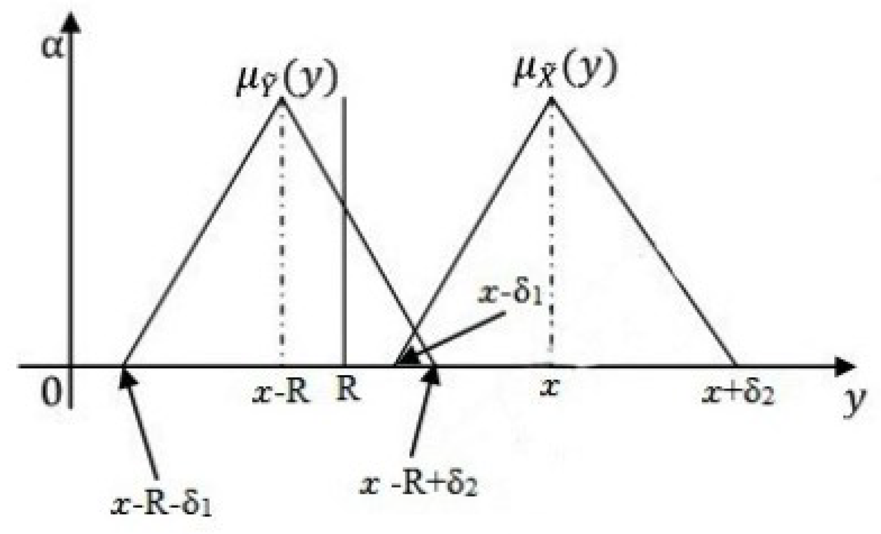
Situation 2: $x\in [R,R+{\delta }_1)$, i.e., $x-R-{\delta }_1<0\mathrm{and}x-R\ge 0$. Figure 3 shows the fuzzy shortage quantity $\tilde{Y}$.

The membership function ${\mu }_{\tilde{Y}}$ of $\tilde{Y}$ is:

$${\mu }_{\tilde{Y}}\left(y\right)=\left\{\begin{array}{cc}{\displaystyle \frac{y-(x-R-{\delta }_1)}{{\delta }_1}},\hfill & 0\le y\le x-R\hfill \\ {\displaystyle \frac{(x-R+{\delta }_2)-y}{{\delta }_2}},\hfill & x-R\le y\le x-R+{\delta }_2\hfill \\ 0,\hfill & \mathrm{otherwise},\hfill \end{array}\right.$$

where $\alpha$-cut $\left[{\tilde{Y}}_{\alpha }^{-},{\tilde{Y}}_{\alpha }^{+}\right]=\left\{\begin{array}{cc}\left[0,x-R+{\delta }_2-\alpha {\delta }_2\right],\hfill & x\in \left[R,R+{\delta }_1-\alpha {\delta }_1\right];\hfill \\ \left[x-R-{\delta }_1+\alpha {\delta }_1,x-R+{\delta }_2-\alpha {\delta }_2\right];\hfill & x\in \left[R+{\delta }_1-\alpha {\delta }_1,R+{\delta }_1\right].\hfill \end{array}\right.$ The expectation of the random interval above is:

$$\left[E[{\tilde{Y}}_{\alpha }^{-}],E[{\tilde{Y}}_{\alpha }^{+}]\right]=\left\{\begin{array}{c}\left[0,{\int }_R^{R+{\delta }_1-\alpha {\delta }_1}(x-R+{\delta }_2-\alpha {\delta }_2)dF\left(x\right)\right]\hfill \\ \left[{\int }_{R+{\delta }_1-\alpha {\delta }_1}^{R+{\delta }_1}(x-R-{\delta }_1+\alpha {\delta }_1)dF\left(x\right),{\int }_{R+{\delta }_1-\alpha {\delta }_1}^{R+{\delta }_1}(x-R+{\delta }_2-\alpha {\delta }_2)dF\left(x\right)\right]\hfill \end{array}\right.$$

(18)

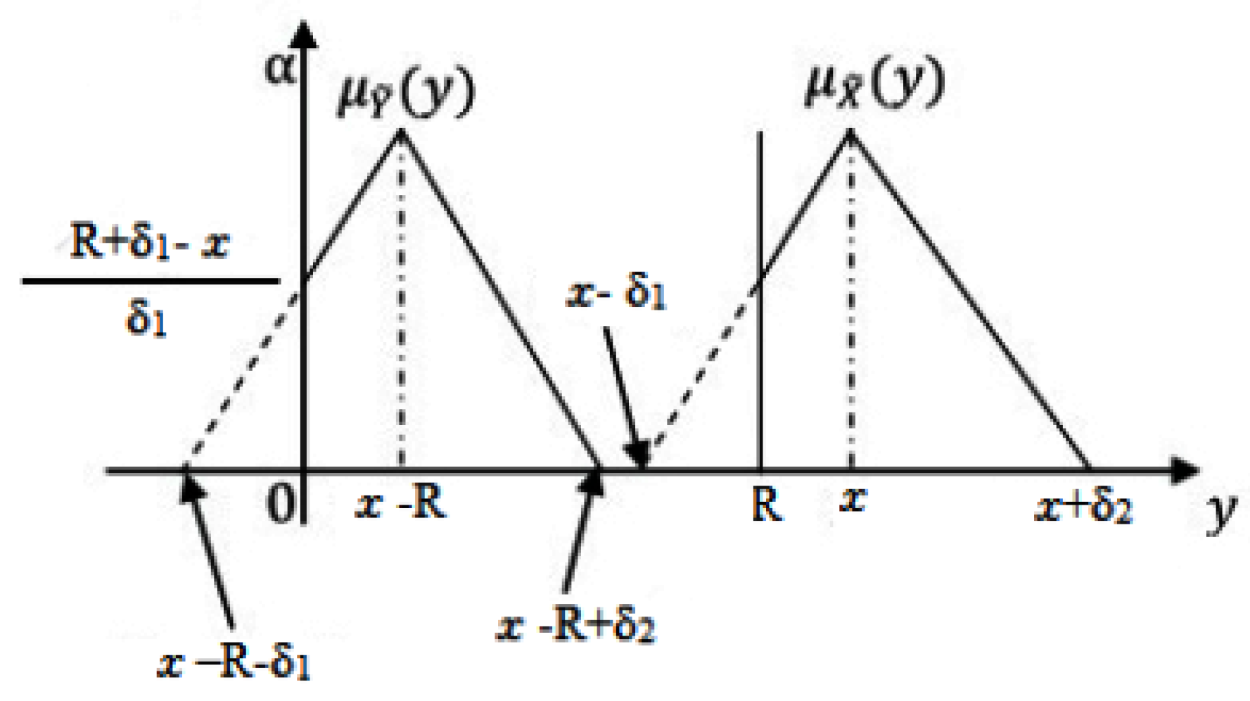
Situation 3: $x\in [R-{\delta }_2,R)$, i.e., $x-R+{\delta }_2\ge 0\mathrm{and}x-R<0$. Figure 4 shows the fuzzy shortage quantity $\tilde{Y}$.

The membership function ${\mu }_{\tilde{Y}}$ of $\tilde{Y}$ is:

$${\mu }_{\tilde{Y}}\left(y\right)=\left\{\begin{array}{cc}{\displaystyle \frac{(x-R+{\delta }_2)-y}{{\delta }_2}},\hfill & 0\le y\le x-R+{\delta }_2\hfill \\ 0,\hfill & \mathrm{otherwise},\hfill \end{array}\right.$$

where $\alpha$-cut $[{\tilde{Y}}_{\alpha }^{-},{\tilde{Y}}_{\alpha }^{+}]=\left\{\begin{array}{cc}[0,0],\hfill & x\in [R-{\delta }_2,R+{\delta }_2-\alpha {\delta }_2];\hfill \\ \left[0,x-R+{\delta }_2-\alpha {\delta }_2\right],\hfill & x\in [R+{\delta }_2-\alpha {\delta }_2,R].\hfill \end{array}\right.$ The expectation of the random interval in this situation is:

$$\left[E[{\tilde{Y}}_{\alpha }^{-}],E[{\tilde{Y}}_{\alpha }^{+}]\right]=\left[0,{\int }_{R-{\delta }_2+\alpha {\delta }_2}^R(x-R+{\delta }_2-\alpha {\delta }_2)dF\left(x\right)\right]$$

(19)

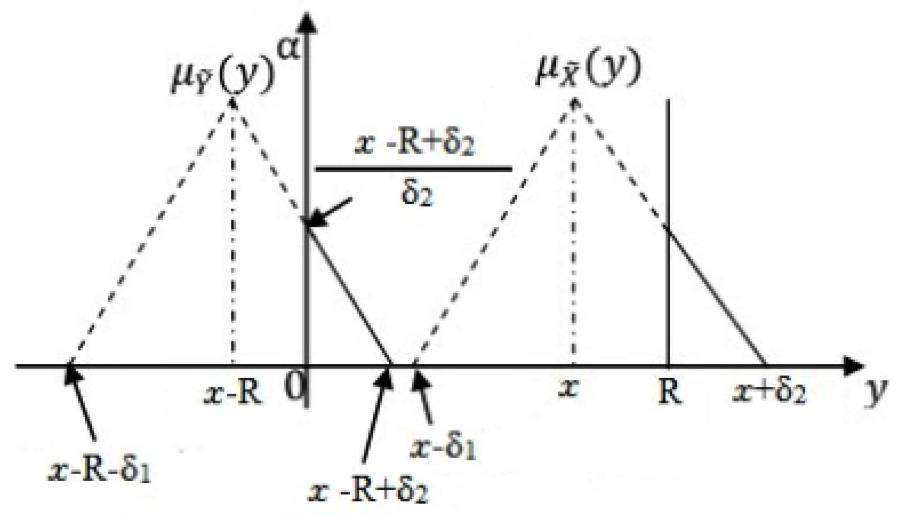
Situation 4: $x\in (-\infty ,R-{\delta }_2)$, i.e., $x-R+{\delta }_2<0$. In this situation, there is no shortage quantity, as shown in Figure 5.

Obviously, the membership function of $\tilde{Y}$ is zero for all y. Consequently, $\left[E[{\tilde{Y}}_{\alpha }^{-}],E[{\tilde{Y}}_{\alpha }^{+}]\right]=[0,0]$. Combining Equations (17)–(19), the $\alpha$-cut of the expectation of the FRV, $\tilde{Y}$, is given by:

$$\begin{array}{cc}\hfill \left[E\left[{\tilde{Y}}_{\alpha }^{-}\right],E\left[{\tilde{Y}}_{\alpha }^{+}\right]\right]=& [{\int }_{R+{\delta }_1-\alpha {\delta }_1}^{\infty }(x-R-{\delta }_1+\alpha {\delta }_1)dF\left(x\right),\hfill \\ & {\int }_{R-{\delta }_2+\alpha {\delta }_2}^{\infty }(x-R+{\delta }_2-\alpha {\delta }_2)dF\left(x\right)]\hfill \end{array}$$

(20)

Now, using the above lemma, the maximum value of the $\alpha$-cut of $E[\tilde{Y}]$ for $0\le \alpha \le 1$ can be calculated as follows:

$$\begin{array}{ccc}& & {\int }_{R+{\delta }_1-\alpha {\delta }_1}^{\infty }(x-R-{\delta }_1+\alpha {\delta }_1)dF\left(x\right)=E{[x-(R+{\delta }_1-\alpha {\delta }_1)]}^{+}\hfill \\ & \le & {\displaystyle \frac{\sqrt{{\sigma }_L^2+{(R+{\delta }_1-\alpha {\delta }_1-d_L)}^2}-(R+{\delta }_1-\alpha {\delta }_1-d_L)}{2}}=U_1(R,L;\alpha )\left(\mathrm{say}\right)\hfill \\ \hfill \end{array}$$

(21)

and

$$\begin{array}{ccc}& & {\int }_{R-{\delta }_2+\alpha {\delta }_2}^{\infty }(x-R+{\delta }_2-\alpha {\delta }_2)dF\left(x\right)=E{[x-(R-{\delta }_2+\alpha {\delta }_2)]}^{+}\hfill \\ & \le & {\displaystyle \frac{\sqrt{{\sigma }_L^2+{(R-{\delta }_2+\alpha {\delta }_2-d_L)}^2}-(R-{\delta }_2+\alpha {\delta }_2-d_L)}{2}}=U_2(R,L;\alpha )\left(\mathrm{say}\right)\hfill \\ \hfill \end{array}$$

(22)

Now, from Equations (16), (21), and (22), the deterministic cost function equivalent to the fuzzy expected cost is as follows:

$$\begin{array}{ccc}\hfill \widetilde{FPVC}(Q,R,L)& \le & \frac{1}{2}{\int }_0^1\left[{\displaystyle \frac{\left[A\left(L\right)+C\left(L\right)\right]}{1-e^{-\theta Q/(D-(1-\alpha ){\Delta }_i)}}}\right]d\alpha \hfill \\ & +& \frac{1}{2}{\int }_0^1\left[{\displaystyle \frac{\left[s+\pi (1-\tau )\right]U_1(R,L;\alpha )}{1-e^{-\theta Q/(D-(1-\alpha ){\Delta }_i)}}}\right]d\alpha \hfill \\ & +& \frac{h}{2\theta }{\int }_0^1\left[R-d_L-(1-\alpha ){\delta }_2+(1-\tau )U_1(R,L;\alpha )\right]d\alpha \hfill \\ & +& \frac{1}{2}{\int }_0^1\left[{\displaystyle \frac{hP(1-e^{-\theta Q/P})}{{\theta }^2(1-e^{-\theta Q/(D-(1-\alpha ){\Delta }_i)})}}+{\displaystyle \frac{hP(1-e^{-\theta Q/P})}{{\theta }^2(1-e^{-\delta Q/(D+(1-\alpha ){\Delta }_i^{\prime })})}}\right]d\alpha \hfill \\ & -& {\displaystyle \frac{1}{2}}{\int }_0^1{\displaystyle \frac{h}{{\theta }^2}}\left[D+(1-\alpha ){\Delta }_i^{\prime }+D-(1-\alpha ){\Delta }_i\right]d\alpha \hfill \\ & +& \frac{1}{2}{\int }_0^1\left[{\displaystyle \frac{\left[A\left(L\right)+C\left(L\right)\right]}{1-e^{-\theta Q/(D+(1-\alpha ){\Delta }_i^{\prime })}}}\right]d\alpha \hfill \\ & +& \frac{1}{2}{\int }_0^1\left[{\displaystyle \frac{\left[s+\pi (1-\tau )\right]U_2(R,L;\alpha )}{1-e^{-\theta Q/(D+(1-\alpha ){\Delta }_i^{\prime })}}}\right]d\alpha \hfill \\ & +& \frac{h}{2\theta }{\int }_0^1\left[R-d_L+(1-\alpha ){\delta }_1+(1-\tau )U_2(R,L;\alpha )\right]d\alpha \hfill \end{array}$$

Therefore,

$$\begin{array}{cc}\hfill \widetilde{FPVC}(Q,R,L)& ={\displaystyle \frac{\left[A\left(L\right)+C\left(L\right)\right]}{2}}\mathsf{\Gamma }(Q;\alpha )+{\displaystyle \frac{[s+\pi (1-\tau \left)\right]}{2}}\Psi (Q,R,L;\alpha )\hfill \\ \hfill & +{\displaystyle \frac{h}{\theta }}(R-d_L^{\prime })+{\displaystyle \frac{h(1-\tau )}{2\theta }}{U}_3(R,L;\alpha )-{\displaystyle \frac{h(1-\tau )}{2\theta }}(R-d_L^{\prime })\hfill \\ \hfill & +{\displaystyle \frac{hP(1-e^{-\theta Q/P})}{2{\theta }^2}}\mathsf{\Gamma }(Q;\alpha )-{\displaystyle \frac{h}{{\theta }^2}}{D}^{\prime }\hfill \end{array}$$

(23)

Similarly, in the fuzzy sense, we apply the min-max distribution-free process to find the optimum solution of the following form:

$$\underset{Q>0}{\mathrm{Min}}\underset{\mathbf{F}\in \mathcal{F}}{\mathrm{Max}}\widetilde{FPVC}(Q,R,L)$$

where

$$\begin{array}{cc}\hfill \widetilde{FPVC}(Q,R,L)=& {\displaystyle \frac{\left[A\left(L\right)+C\left(L\right)\right]}{2}}\mathsf{\Gamma }(Q;\alpha )+{\displaystyle \frac{[s+\pi (1-\tau \left)\right]}{2}}\Psi (Q,R,L;\alpha )\hfill \\ \hfill +& {\displaystyle \frac{h}{\theta }}(R-d_L^{\prime })+{\displaystyle \frac{h(1-\tau )}{2\theta }}{U}_3(R,L;\alpha )-{\displaystyle \frac{h(1-\tau )}{2\theta }}(R-d_L^{\prime })\hfill \\ \hfill +& {\displaystyle \frac{hP(1-e^{-\theta Q/P})}{2{\theta }^2}}\mathsf{\Gamma }(Q;\alpha )-{\displaystyle \frac{h}{{\theta }^2}}{D}^{\prime }\hfill \\ \hfill \mathrm{over}& \left[\left(Q,R,L\right)|Q>0,R\ge D_L+{\displaystyle \frac{{\Delta }_i^{\prime }-{\Delta }_i}{4}}\right]\hfill \end{array}$$

(24)

It can also be verified that $\widetilde{FPVC(Q,R,L)}$ is a convex function in Q and R by satisfying the second-order sufficient conditions (see Appendix A).

Now, for a global optimal solution, $\frac{\partial \widetilde{FPVC(Q,R,L)}}{\partial Q}=0$ and ${\displaystyle \frac{\partial \widetilde{FPVC(Q,R,L)}}{\partial R}}=0$ for the L of the interval $L\in [L_n,L_0]$. Hence,

$$\begin{array}{cc}\hfill {\displaystyle \frac{h{e}^{-\theta Q/P}}{2\theta }}\mathsf{\Gamma }(Q;\alpha )=& \left[{\displaystyle \frac{\left[A\right(L)+C(L\left)\right]}{2}}+{\displaystyle \frac{hP(1-e^{-\theta Q/P})}{2{\theta }^2}}\right]\hfill \\ \hfill \times & {\int }_0^1\left[\frac{\theta {\mathrm{e}}^{-\frac{\theta Q}{D-\left(1-\alpha \right){\Delta }_i}}}{{\left(V_1(Q;\alpha )\right)}^2(D-\left(1-\alpha \right){\Delta }_i)}\right]d\alpha \hfill \\ \hfill +& \left[{\displaystyle \frac{\left[A\right(L)+C(L\left)\right]}{2}}+{\displaystyle \frac{hP(1-e^{-\theta Q/P})}{2{\theta }^2}}\right]\hfill \\ \hfill \times & {\int }_0^1\left[\frac{\theta {\mathrm{e}}^{-\frac{\theta Q}{D+\left(1-\alpha \right){\Delta }_i^{\prime }}}}{{\left(V_2(Q;\alpha )\right)}^2(D+\left(1-\alpha \right){\Delta }_i^{\prime })}\right]d\alpha \hfill \\ \hfill +& {\displaystyle \frac{[s+\pi (1-\tau \left)\right]}{2}}{\int }_0^1\left[\frac{\theta U_1(R,L;\alpha ){\mathrm{e}}^{-\frac{\theta Q}{D-\left(1-\alpha \right){\Delta }_i}}}{{\left(V_1(Q;\alpha )\right)}^2(D-\left(1-\alpha \right){\Delta }_i)}\right]d\alpha \hfill \\ \hfill +& {\displaystyle \frac{[s+\pi (1-\tau \left)\right]}{2}}{\int }_0^1\left[\frac{\theta U_2(R,L;\alpha ){\mathrm{e}}^{-\frac{\theta Q}{D+\left(1-\alpha \right){\Delta }_i^{\prime }}}}{{\left(V_2(Q;\alpha )\right)}^2(D+\left(1-\alpha \right){\Delta }_i^{\prime })}\right]d\alpha \hfill \end{array}$$

(25)

and

$$\begin{array}{cc}\hfill -\frac{h(1+\tau )}{2\theta }=& {\displaystyle \frac{[s+\pi (1-\tau \left)\right]}{2}}{\int }_0^1\left[\frac{V_1(Q;\alpha )}{2}\left({\displaystyle \frac{R+{\delta }_1-\alpha {\delta }_1-d_L}{\sqrt{{\sigma }^{2}L+{(R+{\delta }_1-\alpha {\delta }_1-d_L)}^2}}}-1\right)\right]d\alpha \hfill \\ \hfill +& {\displaystyle \frac{[s+\pi (1-\tau \left)\right]}{2}}{\int }_0^1\left[\frac{V_2(Q;\alpha )}{2}\left({\displaystyle \frac{R-{\delta }_2+\alpha {\delta }_2-d_L}{\sqrt{{\sigma }^{2}L+(R-{\delta }_2+\alpha {\delta }_2-d_L}{)}^2}}-1\right)\right]d\alpha \hfill \\ \hfill +& \frac{h(1-\tau )}{2\theta }{\int }_0^1\left[{\displaystyle \frac{R+{\delta }_1-\alpha {\delta }_1-d_L}{\sqrt{{\sigma }^{2}L+{(R+{\delta }_1-\alpha {\delta }_1-d_L)}^2}}}\right]d\alpha +\frac{h(1-\tau )}{2\theta }\hfill \\ \hfill \times & {\int }_0^1\left[{\displaystyle \frac{R-{\delta }_2+\alpha {\delta }_2-d_L}{\sqrt{{\sigma }^{2}L+(R-{\delta }_2+\alpha {\delta }_2-d_L}{)}^2}}\right]d\alpha \hfill \end{array}$$

(26)

Therefore, from Equation (14), we obtain:

$$\widetilde{FPVC}(Q_f^{\ast },R_f^{\ast },L_f^{\ast })={\displaystyle \frac{\tilde{M}(R_f^{\ast },L_f^{\ast })}{1-e^{-\theta Q_f^{\ast }/\tilde{D}}}}+\tilde{N}(R_f^{\ast },L_f^{\ast })+{\displaystyle \frac{hP}{{\theta }^2}}{\displaystyle \frac{1-e^{-\theta Q_f^{\ast }/P}}{1-e^{-\theta Q_f^{\ast }/\tilde{D}}}}$$

(27)

Using the following algorithm, the fuzzy optimal solution of $(Q,R,L)$ is obtained from Equations (25)–(27). Moreover, the computational procedure is explained to obtain the optimum solution of $(Q,R,L)$, which is denoted by $(Q_f^{\ast },R_f^{\ast },L_f^{\ast })$. An improved Algorithm 2 is developed and presented below.

Algorithm 2: Steps for finding the optimal solution for the fuzzy stochastic model.

Step 1 Input all the parameters.

Step 2 Perform Step 3 to Step 6 for each L from 63 to 21 in reverse order.

Step 3 Calculate $C\left(L\right)$ by crashing components $(p=1,2,\dots ,4)$ from the lowest unit cost to the highest unit cost to have a preparation time of L. For example, $C\left(L\right|63)=0$, $C\left(L\right|62)=0.04$, and so on.

Step 4 Calculate the $A\left(L\right)$ values based on the equation $A\left(L\right)=a_0+a_1{L}^{-\gamma }$, as mentioned in Assumption 1.

Step 5 Find the optimal values of $Q_L^{\ast }$ and $R_L^{\ast }$ and the $PVC(Q,R,L)$ value for the parametric value of L, as mentioned in Step 2, by minimizing $PVC(Q,R,L)$, as developed in Equation (27).

Step 6 Calculate the $SS$ values based on R and L.

Step 7 Select the ($Q_f^{\ast }$, $R_f^{\ast }$, $L_f^{\ast }$) corresponding to the lowest value of $PVC(Q,R,L)$.

Step 8 Present all the required outputs.

3. Numerical Illustration

3.1. Input Parameters

To illustrate the two inventory models developed in the previous section and demonstrate the solution methods described in Algorithms 1 and 2, the following parametric values are considered as presented in

Table 3. Input parameters.

Parameters	Value
Expected annual demand (D)	10,000
Annual production rate (P)	50,000
Replenishment preparation time (L)	63 (days)
Unit holding cost (h)	0.6
Setup time reduction cost (C(L))	0
$(a_0,a_1)$	(60, 10)
Unit shortage cost (s)	1.6
Standard deviation $\left(\sigma \right)$ of demand during the preparation time	$\sqrt{800}$
Proportion of back orders during the stockout period $\left(\tau \right)$	0.5
Interest rate per year $\left(\theta \right)$	0.08
$\gamma$	0.2
$({\Delta }_i,{\Delta }_i^{\prime })$	(1560, 1560)
$D_L$	$\frac{DL}{365}$
$({\Delta }_{L1},{\Delta }_{L2})$	$(\frac{{\Delta }_{i}L}{365},\frac{{\Delta }_i^{\prime }L}{365})$

.

Table 4. Preparation times of different components.

Preparation Time	Normal Duration	Minimum Duration	Unit Crashing
Component p	${\mathit{b}}_{\mathit{r}}$ (Days)	${\mathit{a}}_{\mathit{r}}$ (Days)	Cost ${\mathit{c}}_{\mathit{r}}$ ($/Day)
1	18	4	0.04
2	18	4	0.60
3	13	6	1.90
4	14	7	6.00

presents the data on the production preparation time of four components, which are used for the reduction of preparation time.

3.2. Optimal Solution

The detailed solutions for all possible values of the preparation time $L\in [21,63]$ are evaluated for the stochastic model using Algorithm 1 and the above-mentioned data set.

Table 5. Optimal solution for the stochastic model.

L	$\mathit{A}\left(\mathit{L}\right)$	$\mathit{C}\left(\mathit{L}\right)$	Q	R	$\mathit{SS}$	$\mathit{PVC}(\mathit{Q},\mathit{R},\mathit{L})$
42	64.74	4.76	2273.98	1526.16	375.47	16,639.08
41	64.76	5.36	2273.59	1494.30	371.01	16,602.37
40	64.78	5.96	2273.15	1462.39	366.50	16,564.83
39	64.81	6.56	2272.71	1430.42	361.93	16,526.42
38	64.83	7.16	2272.00	1398.42	357.32	16,487.11
37	64.86	7.76	2271.34	1366.35	352.65	16,446.86
36	64.88	8.36	2270.55	1334.22	347.92	16,405.63
35	64.91	8.96	2269.69	1302.03	343.13	16,363.39
34	64.94	10.86	2281.96	1268.67	337.16	16,392.17
33	64.97	12.76	2293.80	1235.30	331.19	16,419.49
32	65.00	14.66	2305.67	1201.89	325.18	16,445.34
31	65.03	16.56	2317.20	1168.47	319.15	16,469.66
30	65.06	18.46	2328.61	1135.01	313.09	16,492.43
29	65.10	20.36	2339.74	1101.52	306.99	16,513.59
28	65.14	22.26	2350.72	1067.98	300.85	16,533.10

presents the detailed solutions for the preparation time $L\in [28,42]$. The minimum value of $PVC(Q^{\ast },R^{\ast },L^{\ast })$ is found to be $16,363.39 at $L=35$ days with $Q^{\ast }=2269.69$ and $R^{\ast }=1302.03$. Figure 6 shows the cost profile of $PVC(Q,R,L)$ for the preparation time $L=35$ days, and Figure 7 presents the change in order quantity $\left(Q\right)$, reorder point $\left(R\right)$, safety stock $\left(SS\right)$, and $PVC(Q,R,L)$ under different preparation times $\left(L\right)$. Following a similar approach, the detailed solutions for all possible values of the preparation time $L_f\in [21,63]$ are evaluated for the fuzzy stochastic model using Algorithm 2.

Table 6. Optimal solution for the fuzzy stochastic model.

${\mathit{L}}_{\mathit{f}}$	$\mathit{A}\left({\mathit{L}}_{\mathit{f}}\right)$	$\mathit{C}\left({\mathit{L}}_{\mathit{f}}\right)$	${\mathit{Q}}_{\mathit{f}}$	${\mathit{R}}_{\mathit{f}}$	${\left(\mathit{SS}\right)}_{\mathit{f}}$	$\widetilde{\mathit{PVC}}({\mathit{Q}}_{\mathit{f}},{\mathit{R}}_{\mathit{f}},{\mathit{L}}_{\mathit{f}})$
42	64.74	4.76	2321.79	1523.42	372.73	17,699.25
41	64.76	5.36	2321.08	1490.74	367.46	17,643.63
40	64.78	5.96	2320.30	1458.04	362.15	17,587.16
39	64.81	6.56	2319.32	1425.31	356.82	17,529.80
38	64.83	7.16	2318.46	1392.53	351.44	17,471.52
37	64.86	7.76	2317.40	1359.72	346.03	17,412.28
36	64.88	8.36	2316.26	1326.88	340.58	17,352.04
35	64.91	8.96	2314.97	1293.99	335.09	17,290.75
34	64.94	10.86	2326.66	1260.14	328.63	17,299.07
33	64.97	12.76	2337.88	1226.29	322.18	17,305.95
32	65.00	14.66	2348.97	1192.43	315.72	17,311.35
31	65.03	16.56	2359.97	1158.55	309.23	17,315.22
30	65.06	18.46	2370.66	1124.65	302.74	17,317.53
29	65.10	20.36	2381.12	1090.74	296.22	17,318.23
28	65.14	22.26	2391.4	1056.79	289.67	17,317.24

presents the detailed solutions for the preparation time $L_f\in [28,42]$. The minimum value of $\widetilde{PVC}(Q_f^{\ast },R_f^{\ast },L_f^{\ast })$ is found to be $17,290.75 at $L=35$ days with $Q^{\ast }=2314.97$ and $R^{\ast }=1293.99$. Figure 8 presents the cost profile of $\widetilde{PVC}(Q_f,R_f,L_f)$ for the preparation time $L_f=35$ days, and Figure 9 presents the change in order quantity $\left(Q_f\right)$, reorder point $\left(R_f\right)$, safety stock ${\left(SS\right)}_f$, and $\widetilde{PVC}(Q_f,R_f,L_f)$ under different preparation times $\left(L_f\right)$.

3.3. Sensitivity Analysis

3.3.1. Effect of the Holding Cost $\left(H\right)$

To analyze the effect of the holding cost, a sensitivity analysis is carried out by changing the values on both sides (i.e., taking values between 0.40 and 0.80 with an interval of 0.05).

Table 7. Effect of the holding cost in the stochastic and fuzzy stochastic models.

Stochastic Model								Fuzzy Stochastic Model
$\mathit{h}$	$\mathit{L}$	$\mathit{A}\left(\mathit{L}\right)$	$\mathit{C}\left(\mathit{L}\right)$	$\mathit{Q}$	$\mathit{R}$	$\mathit{SS}$	$\mathit{PVC}(\mathit{Q},\mathit{R},\mathit{L})$	${\mathit{L}}_{\mathit{f}}$	$\mathit{A}\left({\mathit{L}}_{\mathit{f}}\right)$	$\mathit{C}\left({\mathit{L}}_{\mathit{f}}\right)$	${\mathit{Q}}_{\mathit{f}}$	${\mathit{R}}_{\mathit{f}}$	${\left(\mathit{SS}\right)}_{\mathit{f}}$	$\widetilde{\mathit{PVC}}({\mathit{Q}}_{\mathit{f}},{\mathit{R}}_{\mathit{f}},{\mathit{L}}_{\mathit{f}})$
0.40	35	64.91	8.96	2716.27	1348.94	390.04	12,953.15	35	64.91	8.96	2768.45	1334.31	375.40	13,611.96
0.45	35	64.91	8.96	2577.68	1334.86	375.96	13,860.52	35	64.91	8.96	2627.73	1322.2	363.30	14,587.72
0.50	35	64.91	8.96	2460.05	1322.58	363.68	14,727.81	35	64.91	8.96	2508.34	1311.65	352.75	15,522.49
0.55	35	64.91	8.96	2358.51	1311.73	352.83	15,560.64	35	64.91	8.96	2405.23	1302.33	343.42	16,422.01
0.60	35	64.91	8.96	2269.69	1302.03	343.13	16,363.39	35	64.91	8.96	2314.97	1293.99	335.09	17,290.75
0.65	35	64.91	8.96	2191.09	1293.28	334.37	17,139.57	35	64.91	8.96	2235.12	1286.46	327.56	18,132.31
0.70	35	64.91	8.96	2120.96	1285.30	326.40	17,892.04	35	65.14	22.26	2232.00	1044.22	277.09	18,940.51
0.75	35	64.91	8.96	2057.80	1278.00	319.10	18,623.17	35	65.14	22.26	2164.41	1038.71	271.59	19,717.70
0.80	35	64.91	8.96	2000.42	1271.28	312.38	19,334.96	35	65.14	22.26	2102.99	1033.65	266.52	20,474.84

presents the detailed outcome of the sensitivity analysis. The expected total cost increases for both models with an increasing holding cost and vice versa. Moreover, the order quantity $\left(Q\right)$ increases substantially as the unit holding cost $\left(h\right)$ decreases, and so do the reorder point and safety stock. The expected total cost and order quantity are lower in the stochastic model than in the fuzzy stochastic model, whereas the reorder point $\left(R\right)$ and safety stock $\left(SS\right)$ are higher in the stochastic model.

3.3.2. Effect of the Shortage Cost $\left(S\right)$

To analyze the effect of the shortage cost, a sensitivity analysis is carried out by changing the values on both sides (i.e., taking values between 0.80 and 2.40 with an interval of 0.20).

Table 8. Effect of the shortage cost in the stochastic and fuzzy stochastic models.

Stochastic Model								Fuzzy Stochastic Model
$\mathit{s}$	$\mathit{L}$	$\mathit{A}\left(\mathit{L}\right)$	$\mathit{C}\left(\mathit{L}\right)$	$\mathit{Q}$	$\mathit{R}$	$\mathit{SS}$	$\mathit{PVC}(\mathit{Q},\mathit{R},\mathit{L})$	${\mathit{L}}_{\mathit{f}}$	$\mathit{A}\left({\mathit{L}}_{\mathit{f}}\right)$	$\mathit{C}\left({\mathit{L}}_{\mathit{f}}\right)$	${\mathit{Q}}_{\mathit{f}}$	${\mathit{R}}_{\mathit{f}}$	${\left(\mathit{SS}\right)}_{\mathit{f}}$	$\widetilde{\mathit{PVC}}({\mathit{Q}}_{\mathit{f}},{\mathit{R}}_{\mathit{f}},{\mathit{L}}_{\mathit{f}})$
0.80	35	64.91	8.96	2186.09	1241.62	282.72	15,415.01	35	64.91	8.96	2221.96	1242.55	283.64	16,269.58
1.00	35	64.91	8.96	2208.39	1258.19	299.28	15,671.40	35	64.91	8.96	2246.78	1256.71	297.81	16,545.34
1.20	35	64.91	8.96	2229.86	1273.66	314.75	15,913.70	35	64.91	8.96	2270.52	1269.91	311.00	16,806.15
1.40	35	64.91	8.96	2250.17	1288.24	329.33	16,143.85	35	64.91	8.96	2293.20	1282.29	323.39	17,054.08
1.60	35	64.91	8.96	2269.69	1302.03	343.13	16,363.39	35	64.91	8.96	2314.97	1293.99	335.09	17,290.75
1.80	35	64.91	8.96	2288.40	1315.15	356.24	16,573.57	35	64.91	8.96	2335.93	1305.09	346.19	17,517.48
2.00	35	64.91	8.96	2306.54	1327.65	368.75	16,775.39	28	65.14	22.26	2427.03	1076.50	309.38	17,710.24
2.20	35	64.91	8.96	2324.05	1339.62	380.72	16,969.71	28	65.14	22.26	2443.92	1085.71	318.59	17,895.92
2.40	35	64.91	8.96	2340.97	1351.12	392.21	17,157.25	28	65.14	22.26	2460.29	1094.56	327.43	18,075.30

presents the detailed outcome of the sensitivity analysis. The expected total cost increases for both models with an increasing shortage cost and vice versa. Moreover, the order quantity $\left(Q\right)$ increases substantially as the unit shortage cost $\left(s\right)$ increases. The expected total cost and order quantity are lower in the stochastic model than in the fuzzy stochastic model, whereas the reorder point $\left(R\right)$ and safety stock $\left(SS\right)$ are higher in the stochastic model as the shortage cost $\left(s\right)$ increases.

3.3.3. Effect of the Back Order Cost $\left(\tau \right)$

Similarly, a sensitivity analysis is performed on the back order cost by changing the values on both sides (i.e., taking values between 0.30 and 0.70 with an interval of 0.05).

Table 9. Effect of the back order cost in the stochastic and fuzzy stochastic models.

Stochastic Model							Fuzzy Stochastic Model
$\mathit{\tau }$	$\mathit{L}$	$\mathit{A}\left(\mathit{L}\right)$	$\mathit{C}\left(\mathit{L}\right)$	$\mathit{Q}$	$\mathit{R}$	$\mathit{SS}$	$\mathit{PVC}(\mathit{Q},\mathit{R},\mathit{L})$	${\mathit{L}}_{\mathit{f}}$	$\mathit{A}\left({\mathit{L}}_{\mathit{f}}\right)$	$\mathit{C}\left({\mathit{L}}_{\mathit{f}}\right)$	${\mathit{Q}}_{\mathit{f}}$	${\mathit{R}}_{\mathit{f}}$	${\left(SS\right)}_f$	$\widetilde{\mathit{PVC}}({\mathit{Q}}_{\mathit{f}},{\mathit{R}}_{\mathit{f}},{\mathit{L}}_{\mathit{f}})$
0.30	35	64.91	8.96	2303.99	1329.76	370.86	16,802.46	28	65.14	22.26	2443.14	1065.83	298.71	17,992.66
0.35	35	64.91	8.96	2295.57	1323.08	364.18	16,696.10	28	65.14	22.26	2430.23	1063.80	296.67	17,825.20
0.40	35	64.91	8.96	2287.15	1316.23	357.33	16,587.55	28	65.14	22.26	2417.39	1061.61	294.49	17,656.85
0.45	35	64.91	8.96	2278.48	1309.22	350.32	16,476.70	35	64.91	8.96	2329.99	1296.60	337.70	17,484.30
0.50	35	64.91	8.96	2269.69	1302.03	343.13	16,363.39	35	64.91	8.96	2314.97	1293.99	335.09	17,290.75
0.55	35	64.91	8.96	2260.75	1294.64	335.74	16,247.49	35	64.91	8.96	2299.90	1291.19	332.28	17095.92
0.60	35	64.91	8.96	2251.61	1287.05	328.15	16,128.80	35	64.91	8.96	2284.78	1288.16	329.26	16,899.70
0.65	35	64.91	8.96	2242.29	1279.24	320.34	16,007.15	35	64.91	8.96	2269.58	1284.90	326.00	16,702.02
0.70	35	64.91	8.96	2232.82	1271.19	312.29	15,882.31	35	64.91	8.96	2254.33	1281.38	322.47	16,502.75

presents the detailed outcome of the sensitivity analysis. The expected total cost decreases for both models with an increasing back order cost and vice versa. Moreover, the order quantity $\left(Q\right)$ increases substantially as the unit back order cost $\left(\tau \right)$ decreases. The expected total cost and order quantity are lower in the stochastic model than in the fuzzy stochastic model, whereas the reorder point $\left(R\right)$ and safety stock $\left(SS\right)$ are higher in the stochastic model.

3.3.4. Effect of the Time Value of Money $\left(\theta \right)$

To analyze the effect of the time value of money, a sensitivity analysis is carried out by changing the values on both sides (i.e., taking values between 0.04 and 0.12 with an interval of 0.01).

Table 10. Effect of the time value of money in the stochastic and fuzzy stochastic models.

Stochastic Model							Fuzzy Stochastic Model
$\mathbf{\theta }$	$\mathit{L}$	$\mathit{A}\left(\mathit{L}\right)$	$\mathit{C}\left(\mathit{L}\right)$	$\mathit{Q}$	$\mathit{R}$	$\mathit{SS}$	$\mathit{PVC}(\mathit{Q},\mathit{R},\mathit{L})$	${\mathit{L}}_{\mathit{f}}$	$\mathit{A}\left({\mathit{L}}_{\mathit{f}}\right)$	$\mathit{C}\left({\mathit{L}}_{\mathit{f}}\right)$	${\mathit{Q}}_{\mathit{f}}$	${\mathit{R}}_{\mathit{f}}$	${\left(\mathit{SS}\right)}_{\mathit{f}}$	$\widetilde{\mathit{PVC}}({\mathit{Q}}_{\mathit{f}},{\mathit{R}}_{\mathit{f}},{\mathit{L}}_{\mathit{f}})$
0.04	35	64.91	8.96	2273.22	1300.84	341.94	32,652.08	35	64.91	8.96	2318.65	1292.98	334.08	34,504.14
0.05	35	64.91	8.96	2272.43	1301.13	342.23	26,136.61	35	64.91	8.96	2317.52	1293.25	334.34	27,618.78
0.06	35	64.91	8.96	2271.44	1301.44	342.53	21,792.95	35	64.91	8.96	2316.82	1293.49	334.58	23,028.54
0.07	35	64.91	8.96	2270.52	1301.74	342.83	18,690.35	35	64.91	8.96	2315.99	1293.73	334.83	19,749.81
0.08	35	64.91	8.96	2269.69	1302.03	343.13	16,363.39	35	64.91	8.96	2314.97	1293.99	335.09	17,290.75
0.09	35	64.91	8.96	2268.93	1302.32	343.41	14,553.54	35	64.91	8.96	2314.02	1294.25	335.34	15,378.16
0.10	35	64.91	8.96	2267.95	1302.62	343.72	13,105.66	35	64.91	8.96	2313.16	1294.49	335.59	13,848.08
0.11	35	64.91	8.96	2267.08	1302.92	344.01	11,921.03	35	64.91	8.96	2312.23	1294.75	335.84	12,596.20
0.12	35	64.91	8.96	2266.21	1303.21	344.31	10,933.84	35	64.91	8.96	2311.32	1295.00	336.10	11,552.97

presents the detailed outcome of the sensitivity analysis. The expected total cost decreases for both models with an increasing $\theta$ and vice versa. Moreover, the order quantity $\left(Q\right)$ increases substantially as $\theta$ decreases. The expected total cost and order quantity are lower in the stochastic model than in the fuzzy stochastic model, whereas the reorder point $\left(R\right)$ and safety stock $\left(SS\right)$ change less as $\theta$ changes.

3.3.5. Effect of $\Delta$

A sensitivity analysis is performed on $\Delta$ (i.e., the percentage change) to study the impact of demand impreciseness in the fuzzy stochastic case.

Table 11. Effect of $\Delta$ in the fuzzy stochastic model.

$\mathsf{\Delta }$	${\mathit{L}}_{\mathit{f}}$	$\mathit{A}\left({\mathit{L}}_{\mathit{f}}\right)$	$\mathit{C}\left({\mathit{L}}_{\mathit{f}}\right)$	${\mathit{Q}}_{\mathit{f}}$	${\mathit{R}}_{\mathit{f}}$	${\left(\mathit{SS}\right)}_{\mathit{f}}$	$\widetilde{\mathit{PVC}}({\mathit{Q}}_{\mathit{f}},{\mathit{R}}_{\mathit{f}},{\mathit{L}}_{\mathit{f}})$
−40	35	64.91	8.96	2321.70	1272.42	313.51	17,133.62
−30	35	64.91	8.96	2320.20	1276.93	318.03	17,166.16
−20	35	64.91	8.96	2318.63	1282.05	323.15	17,203.30
−10	35	64.91	8.96	2316.82	1287.75	328.85	17,244.88
00	35	64.91	8.96	2314.97	1293.99	335.09	17,290.75
10	35	64.91	8.96	2312.98	1300.75	341.84	17,340.73
20	35	64.91	8.96	2310.86	1307.99	349.08	17,394.66
30	28	65.14	22.26	2386.86	1073.06	305.94	17,439.14
40	28	65.14	22.26	2385.25	1079.18	312.06	17,485.54

presents the solution details, showing that for lower values (i.e., −40 percent to 40 percent) of $\Delta$, the optimal setup time is 35 days, and it becomes 28 days thereafter. With an increasing $\Delta$, the order quantity $\left(Q\right)$ reduces for the same optimal setup time, whereas the reorder point $\left(R\right)$ and safety stock $\left(SS\right)$ increase. The total expected cost in the fuzzy stochastic case increases as $\Delta$ increases.

3.4. Discussion

In the previous section, we observed that the optimal preparation time significantly depends on the components’ attributes, i.e., the amount of reduction in component duration possible, the unit crashing cost. If we closely look at the component details, it can be found that the reduction in preparation time is happening step-wise, i.e., the activity with the lowest unit crashing cost is reduced to the lowest possible duration followed by the next component. In our case, the preparation time comes out to be 35 days, which is 28 days less than the sum of normal activity. At L = 35 days, $C\left(L\right)=8.96$, which indicates that Component 1 and Component 2 are fully exploited through crashing. The effect of preparation time reduction can also be observed in the order quantity and reorder level. As the preparation time decreases, the reorder level decreases and the order quantity increases and vice versa. It may be noted that this result is in sync with the findings of Kumar and Goswami [5]. They carried out a sensitivity analysis on the lead-time and showed that the reorder level increases as the lead-time increases and vice versa. However, our objective is to find the optimal lead-time when a reduction of lead-time is possible through crashing of component time. Moreover, in the previous section, we carried out a sensitivity analysis to understand the effect of parameters such as holding cost, shortage cost, and backorder cost on the solution outcome. With the increasing holding cost the reorder level decreases, and so for the backorder cost. However, with the increasing shortage cost, the reorder level increases.

4. Conclusions

In this study, a stochastic production-inventory model is developed with a varying production preparation time and demand, a partial back order, and lost sales. This model considers the time value of money to find the optimal order quantity, reorder point, and production preparation time, while minimizing the total expected cost. In the stochastic model, the min-max distribution-free approach is applied, and analytical results are derived to identify the optimal solutions. The stochastic model is extended by introducing impreciseness in demand during the preparation time, and the new model is formulated in a fuzzy-stochastic environment. The fuzzy cost function for the second model is defuzzified using the signed distance method. Similar to the stochastic model, analytical results are derived, and an algorithmic procedure is developed to identify the optimal solution for the fuzzy-stochastic model.

A numerical illustration is carried out to demonstrate the developed models, as well as the applicability of these models. It is found that order quantity and total cost are more sensitive towards the lower side of the optimal setup time rather than the higher side. The discount rate is also found to be a sensitive factor, while minimizing the total expected cost. Further, the sensitivity analyses on the key model parameters are performed to show the specific effect on the model.

The following aspects may be considered as limitations of the present study and can be taken up as the future research scope.

• In the present study, the signed distance method is used for defuzzification. However, it would be interesting to examine the outcomes of different defuzzification techniques within the existing settings.
• Demand is considered to be a fuzzy parameter, whereas the consideration of other parameters as fuzzy would make the problem more interesting and complex. Instead of a triangular fuzzy number, other approaches can be applied. It is also important to note that the concept of fuzzy learning in line with Soni and Patel [41] can be explored.
• We can explore the use of meta-heuristic algorithms such as the genetic algorithm, particle swarm optimization, and others to find the solution.