Article

Robust Fractional-Order Control Using a Decoupled Pitch and Roll Actuation Strategy for the I-Support Soft Robot

1
Department of Systems Engineering and Automation, University Carlos III of Madrid, Avda. de la Universidad 30, 28911 Leganés, Madrid, Spain
2
The BioRobotics Institute, Scuola Superiore Sant’Anna, Viale Rinaldo Piaggio 34, 56025 Pontedera, Pisa, Italy
3
Department of Excellence in Robotics and AI, Scuola Superiore Sant’Anna, 56025 Pontedera, Pisa, Italy
*
Author to whom correspondence should be addressed.
Mathematics 2021, 9(7), 702; https://doi.org/10.3390/math9070702
Submission received: 28 February 2021 / Revised: 17 March 2021 / Accepted: 22 March 2021 / Published: 24 March 2021
(This article belongs to the Special Issue Applications of Mathematical Models in Engineering)

Abstract

:
Tip control is a current open issue in soft robotics; therefore, it has received a good amount of attention in recent years. The desirable soft characteristics of these robots turn a well-solved problem in classic robotics, like the end-effector kinematics and dynamics, into a challenging problem. The high redundancy condition of these robots hinders classical solutions, resulting in controllers with very high computational costs. In this paper, a simplification is proposed in the actuation setup of the I-Support soft robot, allowing the use of simple strategies for tip inclination control. In order to verify the proposed approach, inclination step input and trajectory-tracking experiments were performed on a single module of the I-Support robot, resulting in zero output error in all cases, including those where the system was exposed to disturbances. The comparative results of the proposed controllers, a proportional integral derivative (PID) and a fractional order robust (FOPI) controller, validate the feasibility of the proposed approach, showing a clear advantage in the use of the fractional robust controller for the tip inclination control of the I-Support robot compared to the integer order controller.

1. Introduction

Soft robotics is a growing research field which aims to incorporating softness in robotic bodies or in novel end effectors, enabling safe and adaptive interactions [1]. Soft robotics is bio-inspired, since it tries to reproduce the abilities of certain animals, such as worms, snakes or the octopus [2], to move without a rigid skeleton or exoskeleton, exploiting their softness in order to squeeze, and adapt to unstructured environments. The stiffness characteristics of traditional industrial robots were desirable because they enabled the fast, reliable and precise performance of tasks, such as those required in factory lines. Conversely, soft robotics finds application in tasks where safety and adaptability to unstructured environments is of paramount importance [1]. Such tasks include delicate food handling, medical procedures, and assistive tasks.
The compliance which characterizes soft robots, besides granting the desired properties, also introduces challenges from the perspective of modeling and control [3]. The hysteresis of the materials and their high redundancy, due to the virtually infinite number of degrees of freedom (DoF) of soft robots, makes them hard to model with high accuracy. Closed-form equations for describing the dynamics of soft robots are available [4], but are too computationally demanding for efficient use in control. The constant curvature (CC) or the piecewise constant curvature (PCC) approaches [5], which assume either all of the robot’s body, or a number of robot sections, to be circular arcs, are computationally efficient, but tend to fail when the robot is highly nonlinear.
A different approach is to rely on neural networks [6] or reinforcement learning [7] for data-driven modeling of the soft robot. In [6], a dynamic model of a soft robot is learned through supervised learning using an auto-regressive network, and is employed for closed-loop control by model-based reinforcement learning. In [7], a multiagent reinforcement learning approach is used to learn the kinematic model of a robotic arm. A trajectory optimization method is also exploited for open-loop control of dynamic reaching tasks [8]. In [9], it was shown that data-driven models can exploit the retraining of their networks’ weights to accommodate external disturbances. An extensive discussion of the challenges of such platforms can be found in [10]. While these data-driven approaches can accurately capture the nonlinearities of soft robot dynamics, their drawback is that neural networks are black box models which are unfit for the traditional controller design methods usually employed for state-space models.
Due to these limitations, many workspace control strategies applied to soft robots are based on nonlinear model-based controllers or linear model-free controller schemes. In the last case, as no model is available for the controller tuning, different alternatives must be used. For instance, an empirical estimation of the kinematic Jacobian matrix is proposed in [11], and later used in an optimal control scheme. Only the works in [12] propose workspace linear controllers, but use very complex control laws, involving the robot’s Jacobian matrix and its derivative. See [3] for a complete survey on different soft robot control strategies.
Feedback control of nonlinear or time-varying systems has been a challenging problem not just for soft robotics, but since the early nonlinear control attempts at the beginning of the last century. Among the approaches proposed for dealing with nonlinearities, robust control has been extensively used for that purpose. This strategy aims to achieve constant system performance (in the sense of behavior), despite potential plant changes.
Some examples of robust control approaches can be found in [13], where a fractional controller is proposed in the robust control of a soft neck, or in [14], where a fuzzy approach is used to model a nonlinear plant (car steering), proposing an output feedback controller to obtain a robust behavior. Other, more advanced, control strategies have also been used, such as the sliding mode control of a wind turbine generator shown in [15], where a robust behavior is obtained in simulations under the conditions of variable wind-speed inputs and other parameter uncertainties. For a detailed discussion of nonlinear system control problems and possible solutions, see [16].
A desirable feature in robust systems consists of providing a constant overshoot despite changes in the plant parameters (usually the gain). This feature, often called iso-damping in the literature, provides a significant advantage in the control of time-varying or nonlinear systems. Often, this robustness specification is based on Bode’s ideal function (see [17]), which features a flat phase diagram, and thus a constant damping. For instance, in [18], the tuning of a proportional integral derivative (PID) controller based on this flat-phase condition is proposed, showing the benefits of this robust specification in several case studies. A similar approach is found in [19], where a relay test is proposed to find the plant parameters, followed by the application of a tuning method based on the aforementioned condition.
Using that robust specification, a wide range of solutions are possible, from the use of a PID control, as described above, to more advanced strategies. A very interesting approach to the robust control problem is found using fractional calculus. Fractional order controllers (FOCs), based on non-integer-order derivative/integral operators, show greater flexibility in fulfilling the flat-phase condition compared to their integer-order alternatives, while keeping most of their benefits. An extensive review of fractional calculus applications in the field of robust control can be found in [20,21], including system modeling and controller design.
Although many fractional controller definitions have been proposed since the first works in [22], the non-integer-order generalization of the classic PID is generally preferred, probably due to its simple control law and strong similarities with the ubiquitous PID controller, allowing classic design tools to be adapted from integer to fractional exponents.
As described in [23], the fractional order PID (FOPID) controllers defined using Equation (1) are able to provide a robust performance despite plant parameter changes and nonlinearities
F O P I D ( s ) = k p + k i 1 s λ + k d s μ ,
where k p , k i , k d are the controller gains, and λ , μ are the fractional operator orders.
Given its benefits and convenience, the FOPID controllers have received particular attention in recent decades. Approaches using the definition in Equation (1) are found in many works. For instance, in [24], new tuning and auto-tuning methods are proposed for the controller parameters, showing excellent results in the control of real plants, like a water circuit or a servomotor. The same controller is used for the control of a DC motor model in [25], also proposing the possible electronic realization of the system. Again, in [26], an optimization method is proposed for the tuning of the same controller, showing excellent results in the control of a real servomotor system.
In this paper, a fractional-order robust control is proposed for I-Support, an assistive soft robot [27]. The particular cases of proportional integral derivative (PID) and fractional-order proportional integral controller (FOPI) are considered due to their plant and model characteristics. As a novelty, a dynamic model of the plant will be used for the controller tuning, achieving excellent results. This is an important contribution, as similar previous works are based on very complex control laws, while the proposed control scheme is based on simple PID or FOPI controllers.
In the following sections, the robotic platform hardware and the chosen model are described. In order to obtain a suitable model, the robot inputs are redefined, allowing for a direct relationship between the actuation variables and the work-space variables, such as orientation and inclination angles. Then, a plant model is obtained using a recursive least squares (RLS) parameter identification method, as described in [28]. Since the identification is done offline, other, simpler methods could be used, such as least-squares fit; however, given the tuning method proposed, the control strategy might be upgraded to an adaptive scheme, as in the case of [29]. Therefore, a recursive identification algorithm like RLS may have future advantages.
Once a plant model is available, it can be used for controller tuning. According to the iso-m procedure explained in [30], the magnitude, phase and slope of the plant are needed, which can be obtained from the RLS identification. In addition, the system’s behavior must be defined using standard performance specifications, like the damping ratio (phase margin) and peak time (crossover frequency). The resulting controller parameters will be used in the robust control scheme proposed for the I-Support robot. See [30] for details on the method application.
It will be shown that the proposed controllers can track the robot’s end effector configuration in termso f its orientation and inclination angles, and can effectively reject external disturbances, despite inaccuracies in the plant’s model, thanks to the robust fractional order control.

2. Materials and Methods
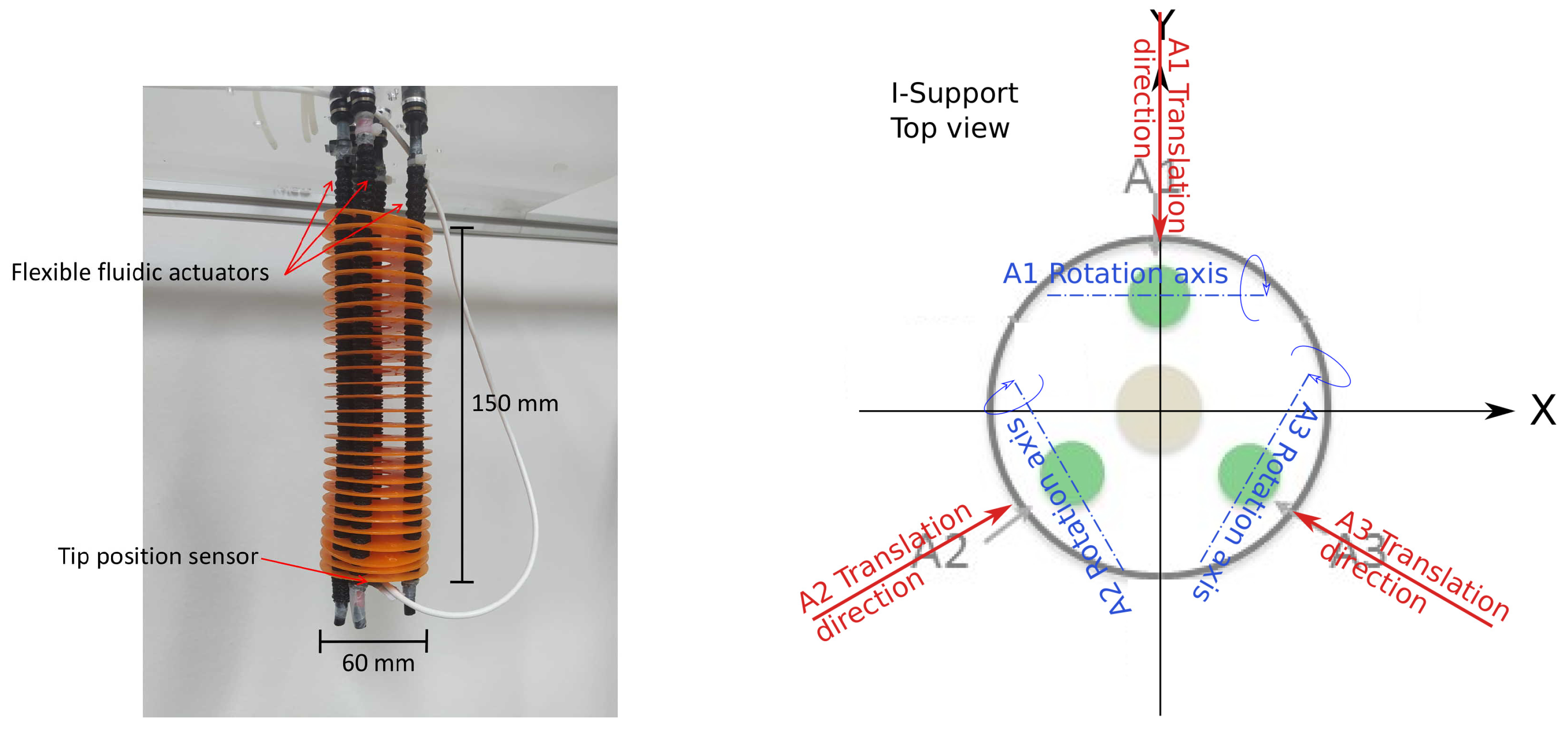
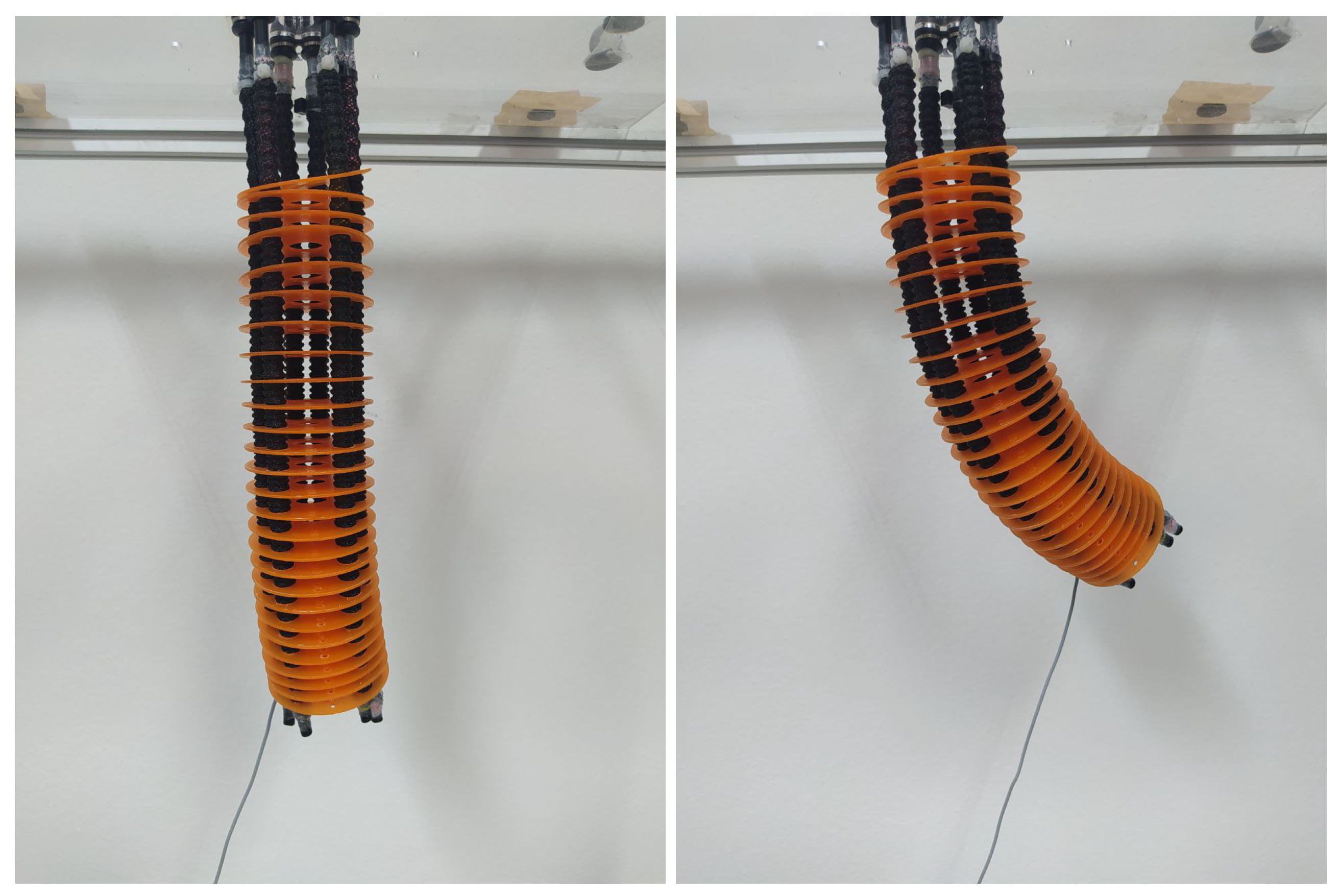
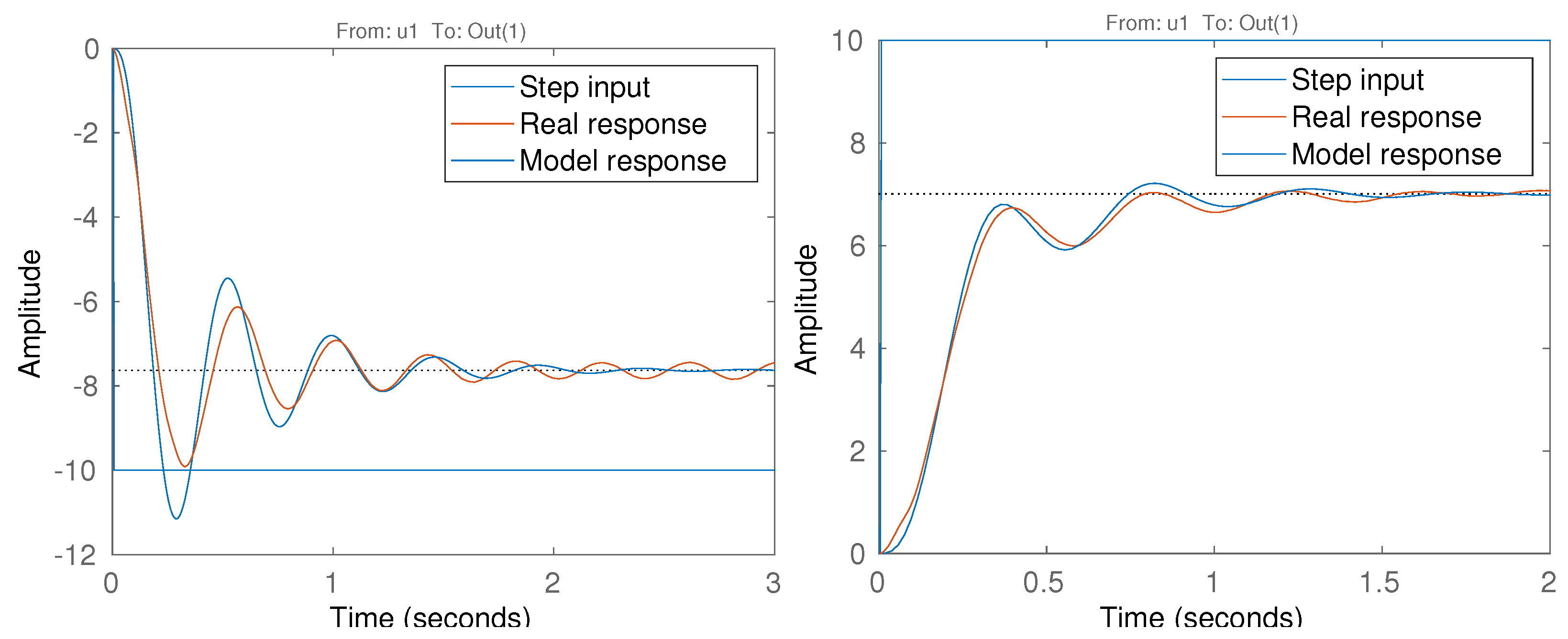
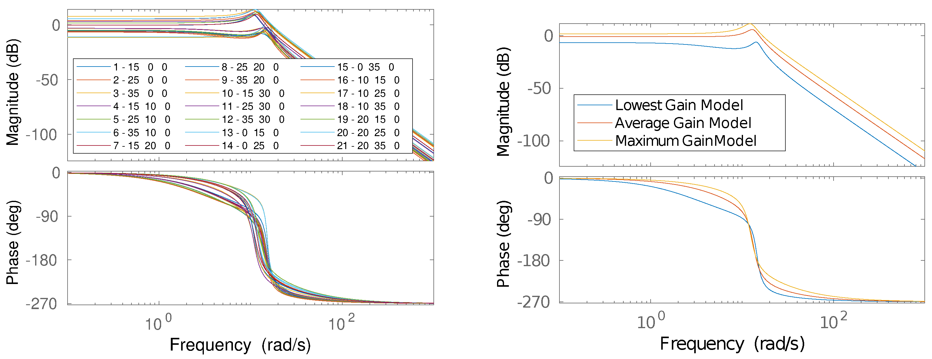
A soft robotic manipulator for the assistance of elderly people, called I-Support, has been used in this work [27] ( Figure 1). It belongs to the class of continuum manipulators that receive inspiration from biological models like elephant trunks or snakes. It is composed of three modules, each of them actuated by three coupled McKibben actuators and three tendon-driven actuators. In this work, the proximal module of the robot was selected and used independently of the others. McKibben actuators are artificial pneumatic muscles, based on an internal latex balloon surrounded by a bellow-shaped braid. The braided structure allows the McKibben actuator to perform uni-directional bending when inflated. The pneumatic actuators are placed within the module at 120° to enable the bending and elongation of the module in all directions. The cable-driven actuation, which was not used in this work for simplicity, allows for shortening and stiffness variation in the module. The McKibben actuators are controlled by Camozzi K8P pneumatic valves, which are controlled by an Arduino Due board. The Arduino is, in turn, controlled by a PC using a serial port within the Matlab environment. The module is kept together by plastic discs placed 10 mm from each other. An internal central channel is built to hold the hose, to provide water and/or soap.

2.1. Plant Model

According to [31,32], this robot is hyper-redundant, making the term degrees of freedom (DOF) not applicable in the classical sense. Nevertheless, in this specific case, the actuation parameters have a direct effect on measurable outputs like tip position and orientation. A correlation between the three available system inputs and the measurable outputs can be found and used to find a plant model.
The I-Support arm module is actuated through three evenly spaced, pressure-driven McKibben pneumatic actuators. As described in [33], the actuator elongation depends on the input pressure, which, in time, produces a change in the position and orientation of the end-effector according to its relative location within the robot. In this case, given the actuator disposition, the different input pressures result in a specific rotation and displacement, depending on the actuator used, as shown in Figure 1. Note that, as there is only one input variable per actuator, its resulting translations and rotations must be bounded.
The combined action of the three actuators produce the final end-effector’s position and orientation in the workspace (Figure 2). As in a three-dimensional environment, the final orientation of the end effector can be defined using three Euler angles. More specifically, in our case, where the rotation in Z axis (yaw) cannot change, the final orientation can be described using two rotation angles in X and Y: pitch and roll. Therefore, the combination of the three angles produced by each actuator will result in a final rotation that can be defined or measured with two angles.
Given that translations and rotations are bound, either can be considered as an output. In this case, end-effector rotations will be considered as the system output. A deeper study of the robot geometry will show how the actuator pressure inputs are related to these final angle outputs.
Starting with a single actuator ( A 1 ), and making its rotation axis parallel to the X axis in the frame of reference (see Figure 1), results in an output angle directly related to the input pressure of its chamber. Given that the angles can be negative, the pressures are also negative for the moment. Although the system does not allow this configuration, it can be solved later by adding an offset. Considering this actuator, with the index number 1, the equations describing angle α in X are as follows
α 1 = f ( P 1 ) .
where α 1 is the angle contribution from the first actuator to the final X axis angle ( α ), P 1 is the actuator input pressure and f is a nonlinear function describing the relationship between them.
However, there are other two actuators with an effect on the final angle α . Given the proposed vertical robot setup, and using the same actuator type at all locations, we can assume that functions f relating the input pressure and actuator angle are also similar. Therefore, the same function applies, but including a projection factor that depends on the actuator relative angle ( γ ), resulting in
α 2 = cos ( γ 2 ) f ( P 2 ) ,
α 3 = cos ( γ 3 ) f ( P 3 ) .
In fact, we can generalize the previous functions as follows
α i = cos ( γ i ) f ( P i ) .
Although the f functions are nonlinear, the resulting tip angles depend on the forces produced by the linear actuators; therefore, given the robot construction, the angles can be considered additive. The final angle in the X axis is then found by addition of the three actuator angles
α = α 1 + α 2 + α 3 = cos ( γ 11 ) f ( P 1 ) + cos ( γ 12 ) f ( P 2 ) + cos ( γ 13 ) f ( P 3 ) .
Since the three actuators are symmetrically arranged, the angles are γ 11 = 0 deg , γ 12 = 120 deg and γ 13 = 240 deg , and Equation (6) results in
α = f ( P 1 ) 0.5 f ( P 2 ) 0.5 f ( P 3 ) = f ( P 1 ) 0.5 [ f ( P 2 ) + f ( P 3 ) ] .
This result shows how both actuators’, A 2 and A 3 , effects on the angle α are divided by two, with an opposite direction to actuator A 1 . This leads to the first result of our approach. The α angle is defined by the pressure difference, which is positive when P 1 is larger than 0.5 ( P 2 + P 3 ) , and negative otherwise. In the case of P 1 = P 2 = P 3 , angle α = 0 , leading to different robot elongations depending on the pressure value, form zero ( P 1 = P 2 = P 3 = 0 ) to full-length ( P 1 = P 2 = P 3 = P m a x ).
Now, β angle is defined as the rotation around Y axis. Using the previous reasoning, but projecting in the Y axis (using sin ( γ ) )
β = β 1 + β 2 + β 3 = sin ( γ 1 ) f ( P 1 ) + sin ( γ 2 ) f ( P 2 ) + sin ( γ 3 ) f ( P 3 ) .
In the case of γ 1 = 0 deg , γ 2 = 120 deg and γ 3 = 240 deg , Equation (8) results in
β = 0.866 f ( P 2 ) 0.866 f ( P 3 ) = 0.866 [ f ( P 2 ) f ( P 3 ) ] .
Note that the value of β angle depends on the difference between P 2 and P 3 , and the effects of the A 1 actuator cannot change it. Again, the angle depends on a pressure difference, and the elongation is a function of the minimum pressure values. For the case P 1 = P 2 = P 3 , angle β = 0 , leading to the previous result regarding robot elongation. As there are just two actuators involved in this case, the final elongation depends on the minimum values between those two pressures.
At this point, we can see that α and β angles depend on the pressure difference of actuators A 1 , A 2 and A 3 , and the elongation depends on the minimum of these values. Based on that, we can define the new input variables β i , α i and l i , as a linear combination of the pressure inputs without loss of generality.
Using the results from Equations (7) and (9), and considering the description for the elongation behavior of the robot, the following input redefinition is proposed
α i = P 1 0.5 ( P 2 + P 3 ) ,
β i = 0.866 ( P 2 P 3 ) ,
l i = min ( P 1 , P 2 , P 3 ) .
As β depends only on the input pressure difference of the actuators A 2 and A 3 , the change in β i will only lead to a change in β output angle. Likewise, α i and l i inputs will affect only the output values of α and l.
Based on thid, the I-Support can be modeled as three decoupled single-input, single-output (SISO) systems. The transfer functions G α , G β , and G l will model the actual outputs ( α , β , l) as a function of the new inputs ( α i , β i , l i ), defined by Equations (10)–(12). Given the simplifications we have considered, the reality will be different in several aspects, such as the interference between actuators and the nonlinear plant behavior, as will be shown in the experimental sections. To deal with these problems, we propose use of a robust controller, since this will provide a constant behavior despite the plant parameter changes or nonlinearities, as discussed above in Section 1.
In order to find these models, recursive least squares (RLS) system identification is proposed. Based on the above discussion, redefined inputs ( α i , β i and l i ) were considered instead of pressure inputs. Note that these are just the pressure input redefinition, and the output angles still depend on the system dynamics. Although f functions are unknown, they are considered within the resulting models, but the nonlinear part will be neglected due to the identification method. As a robust controller is proposed, the performance results will be constant in the entire operation range of the robot, despite these nonlinearities.
As the control system is now defined through angle and elongation inputs, the equivalence between these inputs and the pressure of each actuator is required in order to operate the robot. In that direction, Equations (10) and (11) can be used to solve P 1 and P 2 .
P 2 = β i + P 3 ,
P 1 = α i + 0.5 ( P 2 + P 3 ) = α i + β i 2 + P 3 .
Note that values of P 1 and P 2 depend on α i and β i inputs, and also depend on P 3 , according to Equations (13) and (14). Using these results in Equation (12) provides
l i = min ( α i + β i 2 + P 3 , β i + P 3 , P 3 ) = min ( α i + β i 2 , β i , 0 ) + P 3 ,
where the min function properties are applied to obtain P 3 value out of the min function, leading to the definition of P 3 value based on the inputs α i , β i , and l i detailed in the following equation
P 3 = l i min ( α i + β i 2 , β i , 0 ) .
This result means all the pressure results will be positive as long as l i is greater than zero, which means that this input variable actually controls the robot elongation, as described before.
Once our system is defined, a model is needed for controller tuning and simulation. Given the complex behavior of the robot, system identification is the best option to obtain a linear model from captured data. This means that we neglect the possible nonlinear behavior, but, thanks to the proposed robust controller, a good performance will be obtained despite the model mismatch.
Using the described inputs and outputs definition, a set of experiments were carried out for different target inclinations in order to obtain a plant model. The experimental setup consists of different identification experiments where a changing target was set at one of the three inputs (for instance, α i ), while keeping the other two inputs fixed (for instance, β i , and l i ). A motion-capture system was used to record the real plant behavior, and later used to obtain the output angles ( α and β ) variation.
For example, Figure 3 shows the input and output captured data during two specific identification experiments.
Note that quite different behaviors can be observed for ascending and descending steps. This is probably due to the compressed air valve setting, which can result in plant differences when the air is pushed or released.
A relatively stable output is obtained for the fixed angle, despite the important variations in the changing angle, showing that the systems obtained are mainly decoupled, but a minimal influence still exists. Note that although the input values considered in the identification are α i , β i and l i , the resulting model includes Equations (13), (14) and (16) dynamics (just the linear behavior, of course).
An appropriate number of experiments were performed in the I-Support, covering the entire robot workspace for different input combinations, resulting in a total of 62 separate datasets. Each set consists of the system input data ( α i , β i ) and the response obtained ( α , β ) over a period of 20 s (as shown in Figure 3). Then, RLS identification was applied to selected parts of the captured data, as shown in Figure 4. As expected, the system has an important variation in response over the range of possible inputs. The identification results show how the systems clearly split into two different classes, coincident with the two main observed behaviors. Figure 4 shows a validation example of the RLS results.
Note that although the linear model captures the system behavior quite well, there are mismatches due to plant nonlinearity. In this case, the identification data were extracted from the capture data shown on the left side of Figure 3, but a different identification procedure was performed for every experiment.
Using RLS identification in every dataset will result in a different model for every single experiment. The frequency responses of these models are shown on the left side of Figure 5, using one color label for each identified model, showing experiment number, α i , β i , l. Note that two groups of frequency responses can be observed in the figure. One group shows a decayed resonance with low stationary gain values ( M a g < 0 dB when F r e q 0 rad / s ), and the other group shows a significant resonant peak and higher stationary gain values ( M a g > 0 dB when F r e q 0 rad / s ). These groups are highlighted on the right side of this figure, where only the systems with maximum and minimum gains are shown. In addition, an average model, obtained as the mean value of all resulting RLS parameters, is shown on the right side of Figure 5.
The transfer functions that describe these extreme systems are
G m i n = 311.86 ( s + 3.154 ) ( s 2 + 2.949 s + 210.9 ) , G m a x = 3294.8 ( s + 17.29 ) ( s 2 + 3.382 s + 155.5 ) ,
and the average system transfer function, with poles and gain found as the arithmetic mean of the poles and gain obtained from each dataset, is
G a v g = 1403 ( s + 8.665 ) ( s 2 + 3.462 s + 176.7 ) .
Therefore, two classes can be used to model the I-Support system behavior. One class is the low stationary gain case ( G m i n ), consisting of a pair of complex conjugate poles shaped by the influence of a non-negligible real pole (three dominant poles). The other class shows a higher stationary gain, and is described by ( G m a x ), with two complex dominant poles and one negligible real pole.
The unit input time response and s plane pole locations are shown in Figure 6 for the three described system models. An under-damped behavior is observed for the systems with negligible real poles ( G m a x , G a v g ), while an oscillating over-damped response can be observed in the case with three dominant poles ( G m i n ).
Note how the systems with less than 0 dB gain ( G m i n , G a v g ) show stationary responses below the unit input value, while the other system ( G m a x ) stationary response rises above this input level.
Given these results, a control scheme could be designed using two controllers, one for each system class (two in this case), with a switching supervisor applying the correct controller for each case. Nevertheless, the causes that affect the system behavior are not clear; therefore, the supervisor implementation is not possible in this case. That strategy could be considered in the future if the underlying reason leading to the differences in the plant parameters is found.

2.2. Control Strategy

Considering these conditions, a solution will be proposed using robust control techniques. As discussed before, robust controllers are able to show a constant performance despite plant parameter variations or nonlinearities. Therefore, the average plant parameters can be used for a robust controller tuning, in this way granting an invariant performance in the final system behavior despite changes in the plant parameters (usually gain) or neglected nonlinear plant dynamics.
As discussed in Section 1, the fractional order generalization of the integer order PID controller defined by Equation (1) is a convenient robust control approach, and it is suitable in this case. Given the plant characteristics, the derivative part of the controller is not needed and will only bring noise amplification. Therefore, the fractional order proportional integral (FOPI) variant of the controller, defined by Equation (19), will be used.
F O P I ( s ) = k p + k i 1 s λ .
The three parameters ( k p , k i , λ ) must be tuned in order to achieve the desired system performance. Usual control specifications are stability and responsiveness, normally defined through frequency and damping ratio.
In order to provide a way to compare the robustness between the experiments, a small overshoot will be forced using a target damping ratio lower than 1. As described in [34], a phase margin of 70 deg will result in a damping ratio of 0.8 , enough for a significant overshoot. This allows us to compare the overshoot between experiments, providing a measure of the system robustness by comparison. The design frequency must be low enough to avoid the resonance influence in the vicinity of 10 rad / s in order to enforce stability, with the fastest possible response. Based on this, the performance specifications are the following
  • ϕ m = 70 deg
  • ω g c = 1.5 rad / s
With the defined specifications, several tuning methods are available. The recently published iso-m method, described in [30], is straightforward and easy to apply. In order to tune a fractional order controller, a series of simple operations involving basic math and the use of a graph to find the fractional exponent are needed. Therefore, this method can be applied in the tuning of the controller described in Equation (19).
Using the average model defined in Equation (18) and the iso-m tuning method, the controller parameters shown in Table 1 were found.
Based on these parameters, the resulting controller is defined as follows
F O P I ( s ) = 0.1878 + 1.8279 1 s 1.19 .
An implementation of the fractional operator ( s 1.19 ) is then needed in order to apply the previous controller in the feedback control scheme of the I-Support robot. One of the most common techniques is the equivalent pole-zero approximation described in [35], based on the operator frequency response (see, for example, [24] or [36]). Using that approximation, the s 1.19 operator implementation results in
s 1.19 = 0.6614 s 3 + 1.763 s 2 + 0.4491 s + 0.01586 s 4 + 1.589 s 3 + 0.2861 s 2 + 0.007414 s + 2.53 E 06 .
The frequency response of the open-loop system cascading the controller and the average plant model ( F O P I ( s ) · G a v g ( s ) ), and the closed-loop time response, are shown in Figure 7.
Note that, in the left side of the figure, the phase is completely flat in the vicinity of the crossover frequency, leading to the desired iso-damping property and providing a constant overshoot in the expected step response, shown on the right side of Figure 7.
In a similar way, the same specifications and tuning method were used in an equivalent integer-order controller with the intention of a robustness comparison. The resulting parameters are shown in Table 2.
With these parameters, the resulting controller is
I O P I ( s ) = 0.0071 + 1.6402 1 s .
Again, the frequency and time responses of the system with controller I O P I ( s ) are shown in Figure 8.
See the significant phase slope around the crossover frequency, leading to an important difference in phase margin in the case of a gain change. Although the simulation predicts an underdamped step response, as shown on the right side of Figure 8, in the experimental section, how the overshoot variability is bigger in the case of the integer-order controller will be shown.
A set of experiments were performed for both fractional- and integer-order controllers. The results are shown and discussed in the following section.

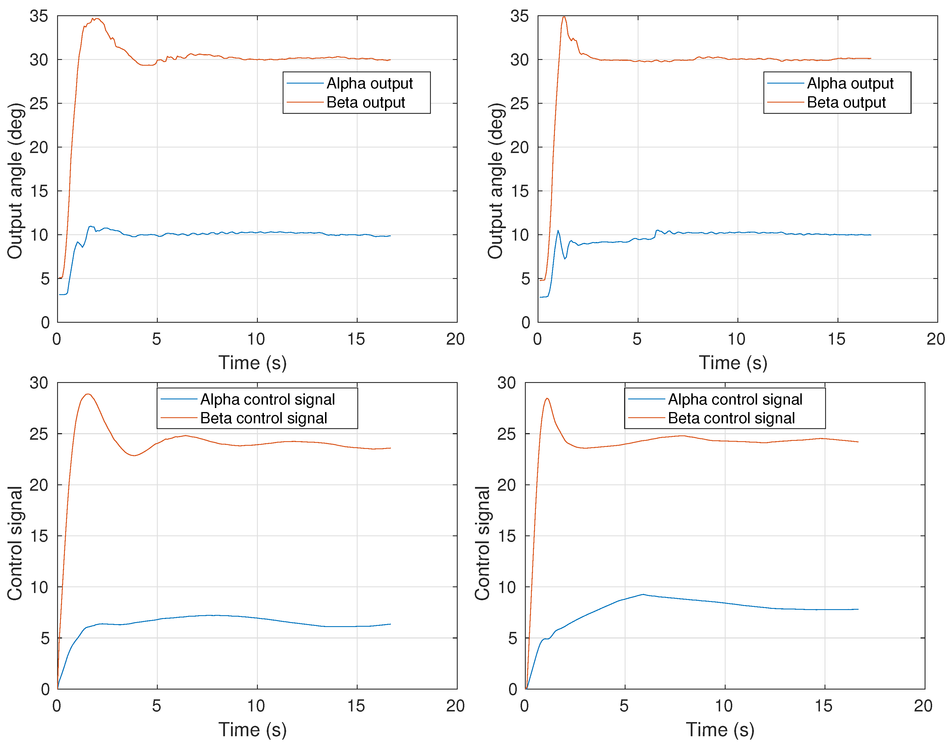
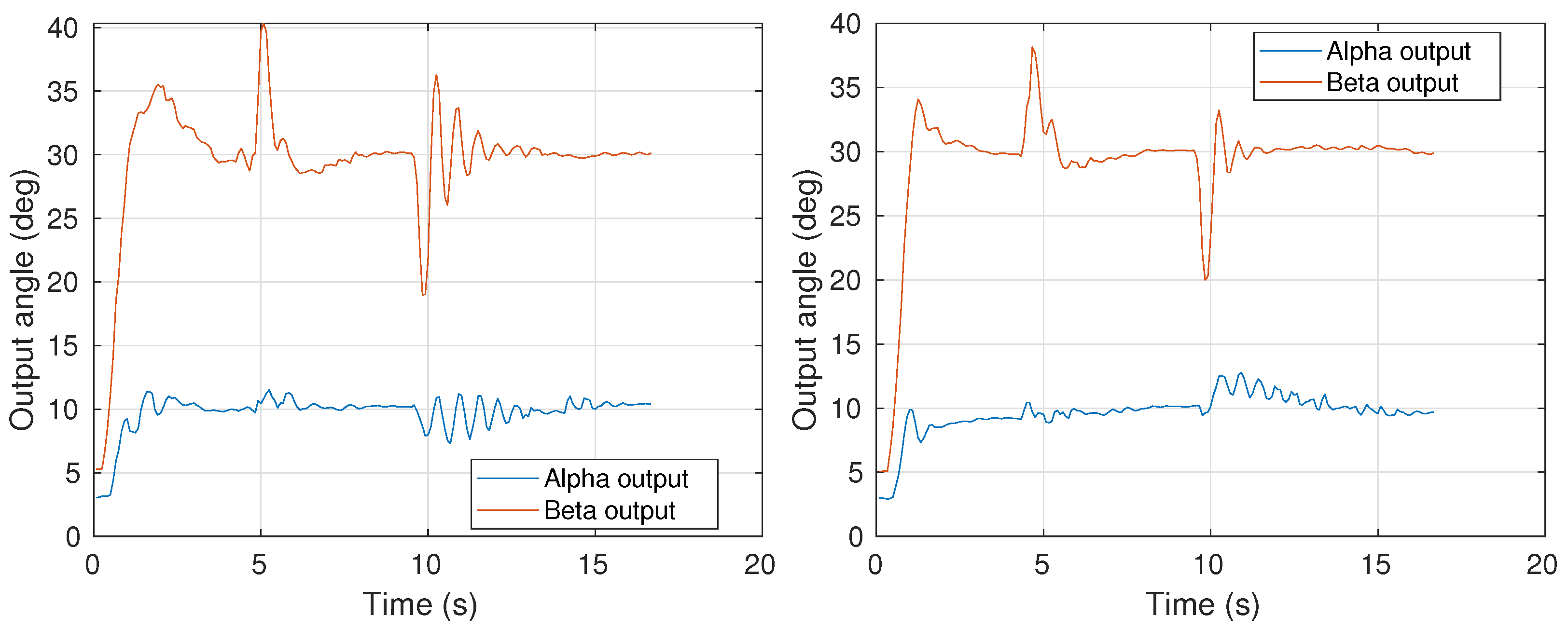
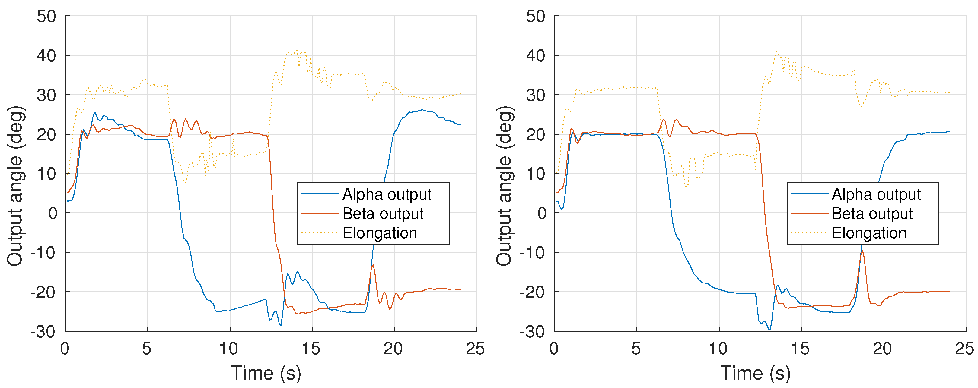
3. Results and Discussion

The experiments performed with the controllers defined in Equations (20) and (22) were designed to assess and compare their performance and robustness properties. As discussed earlier, the goal of robust control is to keep performance characteristics (like overshoot) invariant despite changes in plant parameters (like gain). In this case, we have seen that these parameters change for the different positions attained on the robot and, therefore, a robust system should provide a constant overshoot percentage despite the end effector position changes.
The first experiment consists of exciting the system with two-step input target angles α and β at the same time, showing the controller robustness by overshoot comparison. Tip orientation angles are recorded with an electromagnetic sensor (NDI Aurora®), as shown in Figure 9. Note that a robust system is expected to have the same performance despite plant parameter variations. Given the specifications defined, the difference in overshoot percent values will show the system robustness, with the results showing similar overshoot percentages in both output signals being more robust. An example of this first experiment for target angles α = 10 and β = 30 is shown in Figure 10 for the FOPI and IOPI controllers.
Since the plant parameters change with the inclination, introducing two different references for the target angles ( α = 10 , β = 30 ) allows us to observe the dynamic behavior for two different parameter cases in a single experiment. Observe that, for the fractional-order controller system (left), the overshoot variation is much lower (from 11 % to 16 % ) despite the difference in plant parameters compared to the integer controller (right), which shows a higher overshot difference (from 0 % to 17 % ).
A video recording of this experiment is available at https://vimeo.com/517321273 (accessed on 26 February 2021) for the case of the robust controller, showing the overshoots during the tip positioning and the final controlled angles (Supplementary Material).
The second experiment is a disturbance response test, showing how the control schemes respond to system disturbances. The targets from the first experiment are kept, but, in this case, a constant mass of 150 g is used as a disturbance during the experiment. The setup consists of a metal bar tied to the robot scaffolding in collision with the robot, which can be manually attached or released at any time. In this experiment, the mass was applied at t = 5 s, and removed at t = 10 s, both producing a sudden change in the feedback error, as shown in Figure 11. Disturbance rejection was correct for both controllers.
The third experiment is a trajectory in space describing a square of four targets. This experiment is the most demanding of all the experiments performed, presenting the most extreme parameter variations. In this experiment, a changing reference was programmed, following a trajectory of four positions. The references and points are shown in Table 3.
The results are shown in Figure 12.
Note how the performances are varied in the case of the IOPI controller, ranging from under-damped to over-damped systems, which cannot be considered as robust in the sense described before. In contrast, the FOPI controller keeps a constant performance, showing similar overshoots and time responses during the whole trajectory, which is considered as a robust behavior, known in the literature as iso-damping.
Although elongation input was included to provide larger plant parameter variations, the feedback loop is only applied to orientation control ( α and β ). Therefore, as elongation positions are not feedback-controlled, their results show an important error. The position and elongation control of the I-Support robot will be addressed in future works.

4. Conclusions

A robust control for the I-Support soft robot tip orientation is proposed in this paper through the use of a FOPI controller, and compared to a similar PID controller in terms of performance and robustness.
Given the specific robot characteristics, a previous input variable transformation has been applied in order to split the MIMO system into three decoupled SISO systems. This new approach allows to define the model of each system independently and to apply a different feedback loop to each control variable.
With these decoupled SISO systems defined, a feedback control loop was designed and implemented in these systems, steering the robot tip orientation actuation ( α and β angles). Given the simplifications made in the model, a robust controller is proposed to deal with the parameter variations and neglected dynamics.
The proposed robust control scheme is based on a fractional-order, proportional integral FOPI controller, tuned through a recent method (iso-m) that provides an easy and straightforward solution to the controller parameters. This is considered a major contribution of this paper, as the previous works using similar control strategies show higher control law complexity, resulting in much higher computational costs. This is probably the reason for the restriction of these control strategies to the simulation environment; therefore, none of these works provide experimental results.
Experimentation is then considered as another important contribution of this paper, as a thorough experimental comparison has been carried out between the two proposed controllers in the real I-Support soft robot platform.
The excellent results obtained for the I-Support tip angle control validate the application of this modeling and control scheme and open up the possibilities of position and elongation feedback control of the platform, which will be proposed in future works.
Besides, a further comparison with previous works based on open-loop configuration can be made in the future, to highlight the pros and cons of each control approach and show some hybrid (feedback-machine learning) control possibilities with that can be applied to the I-Support robot or similar platforms.

Supplementary Materials

The following are available online at https://www.mdpi.com/article/10.3390/math9070702/s1.

Author Contributions

Conceptualization, J.M., F.P., C.A.M. and E.F.; methodology, J.M. and F.P.; software, J.M. and F.P.; validation, J.M. and F.P.; formal analysis, J.M.; investigation, J.M. and F.P.; resources, C.A.M. and E.F.; data curation, J.M.; writing—original draft preparation, J.M. and F.P.; writing—review and editing, J.M., F.P., C.A.M. and E.F.; visualization, J.M. and F.P.; supervision, C.A.M. and E.F.; project administration, C.A.M. and E.F.; funding acquisition, C.A.M. and E.F. All authors have read and agreed to the published version of the manuscript.

Funding

The research leading to these results has received funding from the project Desarrollo de articulaciones blandas para aplicaciones robóticas, with reference IND2020/IND-1739, funded by the Comunidad Autónoma de Madrid (CAM) (Department of Education and Research), from HUMASOFT project, with reference DPI2016-75330-P, funded by the Spanish Ministry of Economy and Competitiveness, and from RoboCity2030-DIH-CM, Madrid Robotics Digital Innovation Hub (Robótica aplicada a la mejora de la calidad de vida de los ciudadanos, FaseIV; S2018/NMT-4331), funded by “Programas de Actividades I+D en la Comunidad de Madrid” and cofunded by Structural Funds of the EU. This work was also funded by the European Union’s Horizon 2020 research and innovation programme under grant agreement No. 863212 (PROBOSCIS) and No. 824074 (GROWBOT).

Conflicts of Interest

The authors declare no conflict of interest.

Abbreviations

The following abbreviations are used in this manuscript:
PIDProportional integral derivative
FOPIDFractional order proportional integral derivative
FOPIFractional order proportional integral

References

  1. Kim, S.; Laschi, C.; Trimmer, B. Soft robotics: A bioinspired evolution in robotics. Trends Biotechnol. 2013, 31, 287–294. [Google Scholar] [CrossRef]
  2. Laschi, C.; Cianchetti, M.; Mazzolai, B.; Margheri, L.; Follador, M.; Dario, P. Soft Robot Arm Inspired by the Octopus. Adv. Robot. 2012, 26, 709–727. [Google Scholar] [CrossRef]
  3. George Thuruthel, T.; Ansari, Y.; Falotico, E.; Laschi, C. Control strategies for soft robotic manipulators: A survey. Soft Robot. 2018, 5, 149–163. [Google Scholar] [CrossRef] [PubMed]
  4. Renda, F.; Giorelli, M.; Calisti, M.; Cianchetti, M.; Laschi, C. Dynamic model of a multibending soft robot arm driven by cables. IEEE Trans. Robot. 2014, 30, 1109–1122. [Google Scholar] [CrossRef]
  5. Jones, B.A.; Walker, I.D. Kinematics for multisection continuum robots. IEEE Trans. Robot. 2006, 22, 43–55. [Google Scholar] [CrossRef]
  6. Thuruthel, T.G.; Falotico, E.; Renda, F.; Laschi, C. Model-based reinforcement learning for closed-loop dynamic control of soft robotic manipulators. IEEE Trans. Robot. 2018, 35, 124–134. [Google Scholar] [CrossRef]
  7. Ansari, Y.; Falotico, E.; Mollard, Y.; Busch, B.; Cianchetti, M.; Laschi, C. A Multiagent Reinforcement Learning approach for inverse kinematics of high dimensional manipulators with precision positioning. In Proceedings of the IEEE RAS and EMBS International Conference on Biomedical Robotics and Biomechatronics, Singapore, 26–29 June 2016; pp. 457–463. [Google Scholar]
  8. Thuruthel, T.G.; Falotico, E.; Manti, M.; Laschi, C. Stable Open Loop Control of Soft Robotic Manipulators. IEEE Robot. Autom. Lett. 2018, 3, 1292–1298. [Google Scholar] [CrossRef]
  9. Piqué, F.; Kalidindi, H.T.; Menciassi, A.; Laschi, C.; Falotico, E. A Learning-based Approach for Adaptive Closed-loop Control of a Soft Robotic Arm. In Proceedings of the I-RIM 3D Conference, online, 10–12 December 2020. [Google Scholar]
  10. Della Santina, C.; Bianchi, M.; Grioli, G.; Angelini, F.; Catalano, M.; Garabini, M.; Bicchi, A. Controlling Soft Robots: Balancing Feedback and Feedforward Elements. IEEE Robot. Autom. Mag. 2017, 24, 75–83. [Google Scholar] [CrossRef]
  11. Yip, M.C.; Camarillo, D.B. Model-Less Feedback Control of Continuum Manipulators in Constrained Environments. IEEE Trans. Robot. 2014, 30, 880–889. [Google Scholar] [CrossRef]
  12. Kapadia, A.; Walker, I.D. Task-space control of extensible continuum manipulators. In Proceedings of the 2011 IEEE/RSJ International Conference on Intelligent Robots and Systems, San Francisco, CA, USA, 25–30 September 2011; pp. 1087–1092. [Google Scholar] [CrossRef]
  13. Deutschmann, B.; Ott, C.; Monje, C.A.; Balaguer, C. Robust Motion Control of a Soft Robotic System Using Fractional Order Control. In Advances in Service and Industrial Robotics; Ferraresi, C., Quaglia, G., Eds.; Springer International Publishing: Cham, Switzerland, 2018; pp. 147–155. [Google Scholar] [CrossRef]
  14. Chang, X.H.; Xiong, J.; Park, J.H. Fuzzy robust dynamic output feedback control of nonlinear systems with linear fractional parametric uncertainties. Appl. Math. Comput. 2016, 291, 213–225. [Google Scholar] [CrossRef]
  15. Barambones, O.; Gonzalez de Durana, J.; De la Sen, M. Robust speed control for a variable speed wind turbine. Int. J. Innov. Comput. Inf. Control IJICIC 2010, 8, 7627–7640. [Google Scholar]
  16. Iqbal, J.; Ullah, M.; Khan, S.G.; Khelifa, B.; Ćuković, S. Nonlinear control systems-A brief overview of historical and recent advances. Nonlinear Eng. 2017, 6, 301–312. [Google Scholar] [CrossRef]
  17. Bode, H.W. Network Analysis and Feedback Amplifier Design; Bell Telephone Laboratory Series; Van Nostrand: New York, NY, USA, 1945. [Google Scholar]
  18. Barbosa, R.S.; Machado, J.A.T.; Ferreira, I.M. Tuning of PID Controllers Based on Bode’s Ideal Transfer Function. Nonlinear Dyn. 2004, 38, 305–321. [Google Scholar] [CrossRef]
  19. Chen, Y.; Moore, K.L. Relay Feedback Tuning of Robust PID Controllers with Iso-damping Property. IEEE Trans. Syst. Man Cybern. Part B (Cybern.) 2005, 35, 23–31. [Google Scholar] [CrossRef] [PubMed]
  20. Sabatier, J.; Agrawal, O.P.; Machado, J.A.T. (Eds.) Advances in Fractional Calculus: Theoretical Developments and Applications in Physics and Engineering; Springer: Dordrecht, The Netherlands, 2007. [Google Scholar]
  21. Monje, C.A.; Chen, Y.; Vinagre, B.M.; Xue, D.; Feliu-Batlle, V. Fractional-Order Systems and Controls: Fundamentals and Applications; Springer Science & Business Media: Dordrecht, The Netherlands, 2010. [Google Scholar]
  22. Oustaloup, A. La Dérivation non Entière Théorie, Synthèse et Applications; Hermès: Paris, France, 1995; p. 507. [Google Scholar]
  23. Podlubny, I. Fractional-order systems and PIλDμ-controllers. IEEE Trans. Autom. Control 1999, 44, 208–214. [Google Scholar] [CrossRef]
  24. Monje, C.A.; Vinagre, B.M.; Santamaría, G.E.; Tejado, I. Auto-tuning of fractional order PIλDμ controllers using a PLC. In Proceedings of the 2009 IEEE Conference on Emerging Technologies Factory Automation, Mallorca, Spain, 22–25 September 2009; pp. 1–7. [Google Scholar] [CrossRef]
  25. Petras, I. Fractional order feedback control of a DC motor. J. Electr. Eng. 2009, 60, 117–128. [Google Scholar]
  26. Martín, F.; Monje, C.A.; Moreno, L.; Balaguer, C. DE-based tuning of PIλDμ controllers. ISA Trans. 2015, 59, 398–407. [Google Scholar] [CrossRef]
  27. Manti, M.; Pratesi, A.; Falotico, E.; Cianchetti, M.; Laschi, C. Soft assistive robot for personal care of elderly people. In Proceedings of the 2016 6th IEEE International Conference on Biomedical Robotics and Biomechatronics (BioRob), Singapore, 26–29 June 2016; pp. 833–838. [Google Scholar] [CrossRef]
  28. Ljung, L. Experiments with Identification of Continuous Time Models. IFAC Proc. Vol. 2009, 42, 1175–1180. [Google Scholar] [CrossRef]
  29. Muñoz, J.; Copaci, D.; Monje, C.A.; Blanco, D.; Balaguer, C. Iso-m based adaptive fractional order control with application to a soft robotic neck. IEEE Access 2020, 1. [Google Scholar] [CrossRef]
  30. Muñoz, J.; Monje, C.A.; Nagua, L.F.; Balaguer, C. A graphical tuning method for fractional order controllers based on iso-slope phase curves. ISA Trans. 2020. [Google Scholar] [CrossRef]
  31. Martín Barrio, A.; Terrile, S.; Barrientos, A.; del Cerro, J. Robots Hiper-Redundantes: Clasificación, Estado del Arte y Problemática. Rev. Iberoam. Autom. Inform. Industrial 2018, 15, 351–362. [Google Scholar] [CrossRef]
  32. Martin, A.; Barrientos, A.; del Cerro, J. The Natural-CCD Algorithm, a Novel Method to Solve the Inverse Kinematics of Hyper-redundant and Soft Robots. Soft Robot. 2018, 5, 242–257. [Google Scholar] [CrossRef] [PubMed]
  33. Ansari, Y.; Manti, M.; Falotico, E.; Mollard, Y.; Cianchetti, M.; Laschi, C. Towards the development of a soft manipulator as an assistive robot for personal care of elderly people. Int. J. Adv. Robot. Syst. 2017, 14, 1729881416687132. [Google Scholar] [CrossRef]
  34. Nise, N.S. Frequency response techniques. In Control Systems Engineering; Wiley: Hoboken, NJ, USA, 2019; Chapter 10; pp. 525–612. [Google Scholar]
  35. Levy, E.C. Complex-Curve Fitting. IRE Trans. Autom. Control 1959, AC-4, 37–43. [Google Scholar] [CrossRef]
  36. Valerio, D.; da Costa, J.S. An Introduction to Fractional Control; Control, Robotics and Sensors; Institution of Engineering and Technology: London, UK, 2012. [Google Scholar] [CrossRef]
Figure 1. I-Support kinematic description.
Mathematics 09 00702 g001
Figure 2. Left: elongated I-Support module, with three equally actuated chambers. Right: bended module with only one chamber inflated.
Mathematics 09 00702 g002
Figure 3. Two examples of identification experiments. The left figure shows the system response to variations in the input α i , while the other inputs are kept constant ( β i = 30 and l i = 0 ). Right figure shows the system response to variations in the input β i , while the other inputs are kept constant ( α i = 20 and l i = 0 ).
Mathematics 09 00702 g003
Figure 4. Validation example of the identified models showing two different behaviors. Data obtained from the case of variations in Alpha input ranging from 10 deg to 20 deg (left of Figure 3). Showing the Step input (Alpha input), and the Real response (Alpha output) used in the RLS identification. Resulting model time response is also shown for comparison.
Mathematics 09 00702 g004
Figure 5. Frequency response of the models obtained using RLS, showing all the identification experiments (left) and the three most representative examples: Lowest, Average and Maximum Gains (right).
Mathematics 09 00702 g005
Figure 6. Zero-pole representation (left) and unit input time response (right) for the three most representative models obtained: Lowest Gain ( G m i n ), Average Gain ( G a v g ) and Maximum Gain ( G m a x ) models.
Mathematics 09 00702 g006
Figure 7. Frequency response (left) and time response (right) for the fractional order controller system.
Mathematics 09 00702 g007
Figure 8. Frequency response (left) and time response (right) for the integer order controller system.
Mathematics 09 00702 g008
Figure 9. Experimental setup.
Mathematics 09 00702 g009
Figure 10. Experiment 1. Time response (above) and control signal (below) for the two controllers tested, fractional (left) and integer (right) orders.
Mathematics 09 00702 g010
Figure 11. Experiment 2. Disturbance rejection. Time response for the two controllers tested, fractional (left) and integer (right) orders.
Mathematics 09 00702 g011
Figure 12. Experiment 3. Trajectory tracking. Time response for the two controllers tested, fractional (left) and integer (right) orders.
Mathematics 09 00702 g012
Table 1. Fractional order controller parameters.
k p k i λ
0.1878 1.8279 1.19
Table 2. Integer order controller parameters.
k p k i λ
0.0071 1.6402 1.00
Table 3. Trajectory for experiment 3.
α β l
Point 1202040
Point 2−202020
Point 3−20−2040
Point 420−2020
Publisher’s Note: MDPI stays neutral with regard to jurisdictional claims in published maps and institutional affiliations.

