Evaluation Procedures for Forecasting with Spatiotemporal Data ^†

Abstract

The increasing use of sensor networks has led to an ever larger number of available spatiotemporal datasets. Forecasting applications using this type of data are frequently motivated by important domains such as environmental monitoring. Being able to properly assess the performance of different forecasting approaches is fundamental to achieve progress. However, traditional performance estimation procedures, such as cross-validation, face challenges due to the implicit dependence between observations in spatiotemporal datasets. In this paper, we empirically compare several variants of cross-validation (CV) and out-of-sample (OOS) performance estimation procedures, using both artificially generated and real-world spatiotemporal datasets. Our results show both CV and OOS reporting useful estimates, but they suggest that blocking data in space and/or in time may be useful in mitigating CV’s bias to underestimate error. Overall, our study shows the importance of considering data dependencies when estimating the performance of spatiotemporal forecasting models.

1. Introduction

As sensor networks become widespread, large databases of geo-referenced time series are increasingly available. Machine learning models are needed in order to leverage these data to guide decisions in real-world applications, from air and water quality monitoring [1] to photovoltaic energy production forecasting [2]. These models must be able to produce accurate predictions of future numeric values at multiple geographical locations, but progress in their predictive ability can only be achieved if we can trust our estimations of their performance.

The problem of estimating the performance of any forecasting model on unseen data is, therefore, at the core of predictive analytics. In effect, estimation methods address two relevant challenges faced by analysts: (i) to provide end-users with reliable estimates of the future performance of the models; and (ii) to help analysts in selecting the best possible prediction model from an ever increasing set of available alternatives. Performance estimation involves addressing two questions: (i) which evaluation metrics are an appropriate fit to the application domain; and (ii) how to best use valuable data in order to obtain accurate estimates of these metrics. This paper focuses on the latter question, in the context of forecasting with geo-referenced time series data. The answer is not always obvious. Indeed, standard performance estimation methods such as cross-validation (CV) often assume observations in the training and test sets to be independent [3]. The presence of spatial and temporal autocorrelation means that this assumption will not hold for spatiotemporal data, and it may lead to overly optimistic loss estimates.

Machine learning performance estimation procedures can be classified into two main classes of methods, both widely used: out-of-sample (OOS) estimation and CV strategies.

Hold-out validation is the simplest OOS estimator. It operates by splitting the data into a training set, used to learn a model, and a test set, used to estimate the loss of the learned model in “unseen” data [4]. In forecasting, only OOS procedures that respect the underlying order of the data may be considered (e.g., in data ordered by time, such as time series, the test set is always comprised of the more recent observations). These approaches are sometimes called “last-block” procedures [5].

In CV, the available data are split into several equally sized blocks and these blocks are combined in different ways to generate diverse training sets and test sets. Estimates of performance are obtained by averaging the test-set losses over the several train+test splits [6]. The way the blocks are combined is such that it allows the whole dataset to be used in the test set at least once. The data may be split in an exhaustive or partial manner, with partial splitting often being more computationally viable. The classical example of exhaustive splitting is leave-one-out cross-validation (LOOCV) where each observation plays the role of test set once and is used as part of the training set for all other observations. A common way to partially split the data is to divide them into K subsets of approximately the same size, and then having each subset successively used as test set with all remaining partitions (or folds) used for training—this strategy is referred to as K-fold CV [7]. However, standard CV procedures such as this assume that each test set is independent from the training set, which does not hold for many types of datasets, such as time series [3]. Several variations of CV procedures that do not require independence between sets have been proposed, with most of them being geared toward a time series setting [8,9,10]. Some of these methods have been proposed for spatiotemporal settings [11].

Previous empirical studies about performance estimation methodologies in the presence of dependencies have focused on either temporal [5,12,13,14] or spatial data [15]. Meyer et al. [11] compared three different cross-validation methods for spatiotemporal interpolation. However, to the best of our knowledge, the work [16] we extend in this paper is the first to provide an exhaustive empirical study of both out-of-sample and cross-validation estimation methods for spatiotemporal forecasting tasks.

Our study aims at: (i) providing a review of estimation strategies in the presence of spatiotemporal dependencies; and (ii) investigating how accurately different cross-validation and out-of-sample strategies estimate the predictive performance of models. We perform our study in a geo-referenced time series forecasting setting. Accuracy of error estimates is obtained by comparing the loss estimated by several procedures against the loss measured in previously withheld data acting as a kind of gold standard. In our empirical comparisons, we consider over 15 variations of error estimation procedures, using both artificial and real-world datasets. In this extended version, we report on new experiments using additional artificial data sets and learning models, provide better descriptions of data sets and methods, and present additional analysis and a deeper discussion of our results.

Next, we provide an overview of performance estimation methods that have been proposed for temporal, spatial and spatiotemporal data.

1.1. Performance Estimation with Spatiotemporal Dependence Structures

Observations that have been made at different times and/or at neighbouring locations may be related through internal dependence structures within datasets, as there is a tendency for values of close observations (in terms of either measurement time or location, or both) to be more similar (or otherwise related) than distant ones. This is expected as most measured phenomena have some sort of continuity or smoothness, with abrupt changes being less common or unexpected. For instance, the measured amount of rain at time t on location x is probably correlated with the rain levels at nearby locations or at recent time stamps.

The possibility of dependence among observations may lead to dependence between observations used to train the predictive models and the observations used to test them. This in turn may lead to overly optimistic estimates of the loss a model will incur when presented with previously unseen, independent data, and it may also lead to structural overfitting and poor generalisation ability [15]. In fact, more than one study has proven that CV overfits for choosing the bandwidth of a kernel estimator in regression [17,18].

1.1.1. Temporal Dependence

Several performance estimation methods specifically designed to deal with temporal dependency have been proposed in the past.

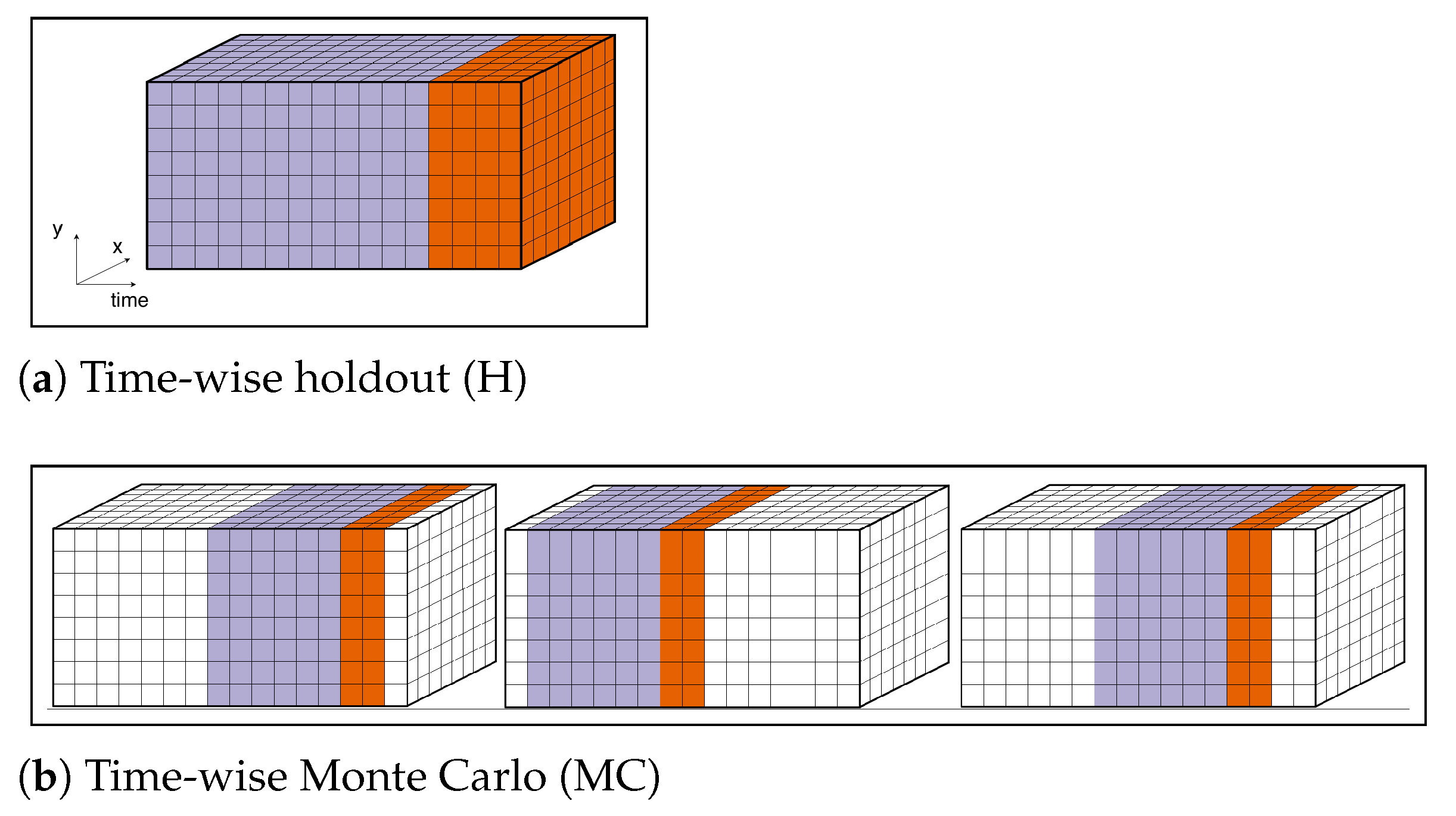
In terms of OOS procedures in time series settings, decisions must be made regarding the split point between training/test sets and how long a time-interval to include in both the training and testing sets. Two approaches are worth mentioning: (a) Repeated time-wise holdout involves repeating a holdout procedure over different periods of time so that loss estimates are more robust, as advised in [19]. The selection of split points for each repetition of holdout may be randomised, with a window of preceding observations used for training and a fraction of the following instances used for testing. Training and test sets may potentially overlap across repetitions, similarly to random sub-sampling. 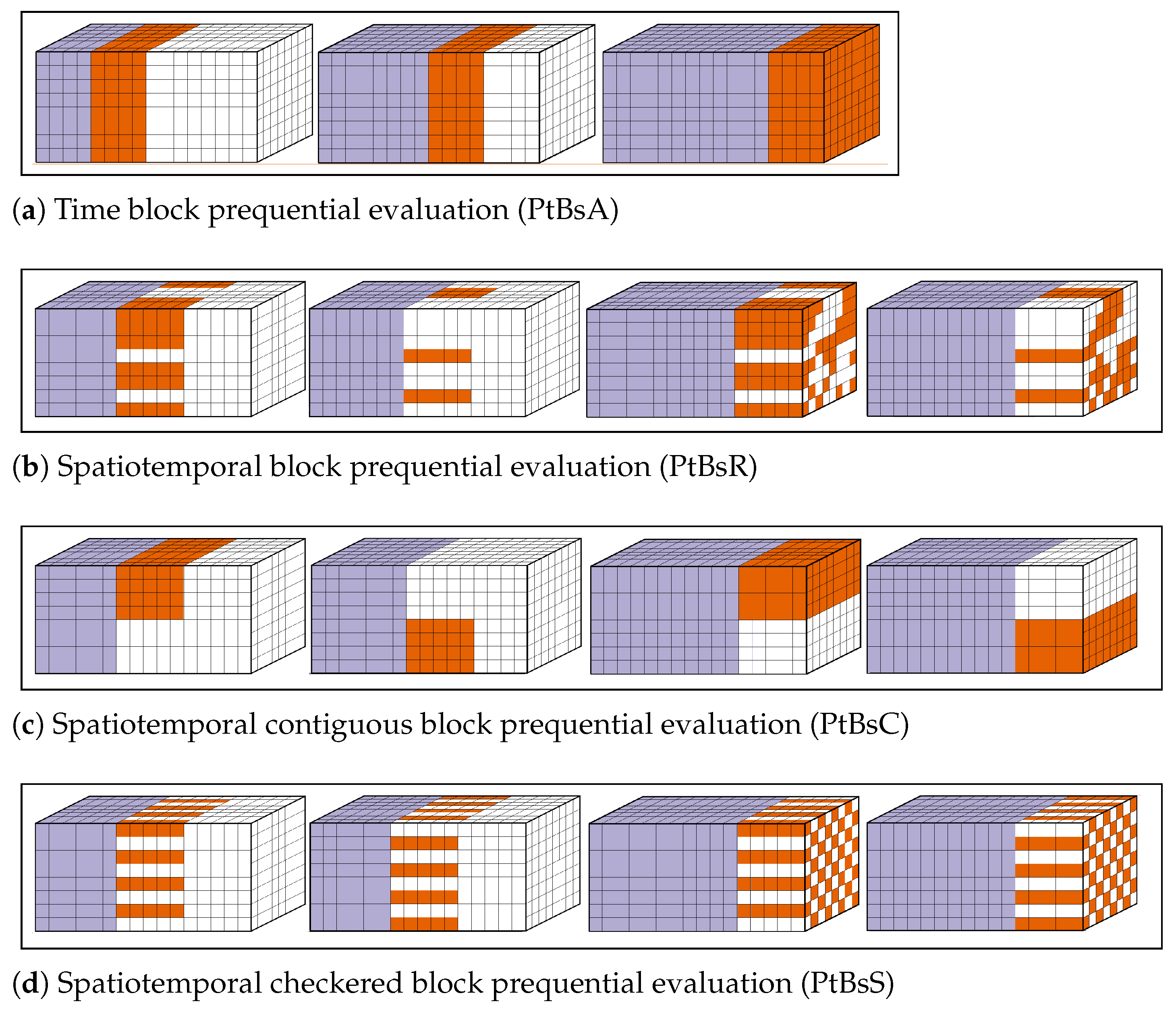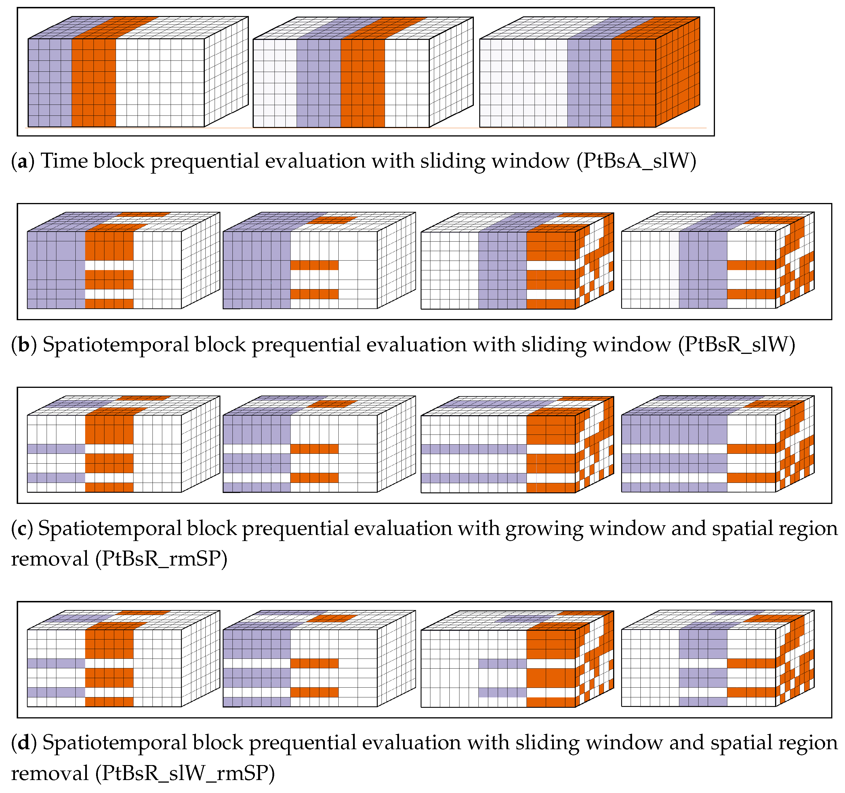These are also referred to as Monte Carlo experiments [20]. (b) Prequential evaluation or interleaved-test-then-train evaluation is often used in data stream mining. Each observation (or block of non-overlapping observations) is first used to test and then to train the model [21] in a sequential manner. The term prequential usually refers to the case where the training window is growing, i.e., a block of observations that is used for testing in one iteration will be merged with all previous training blocks and used for training in the next iteration.

Four alternatives to standard CV proposed for time series should be highlighted: (a) Modified CV is similar to K-fold CV, except that l observations preceding and following the observation(s) in the test set are discarded from the training set after shuffling and fold assignment [8]. This method is also referred to as non-dependent cross-validation in [5]. (b) Block CV is a procedure similar to K-fold CV where, instead of the observations being randomly assigned to folds, each fold is a sequential, non-interrupted time series [22]. (c) h-block CV is based on LOOCV, except h observations preceding and following the observation in the test set are removed from the training set [9]. (d) $hv$-block CV is a modification of h-block CV where, instead of having single observations as test sets, a block of v observations preceding and following each observation is used for testing (causing test sets to overlap), with h observations before and after each block being removed from the training set [10].

Note that, while, in all types of block-CV, each test set is composed of a sequential non-interrupted time series (or a single observation), a fold in modified CV will almost certainly have non-sequential observations. If K is set to the number of observations in modified CV, then it works the same as h-block CV. Moreover, note that only $hv$-block CV allows test sets to overlap.

Several empirical studies have compared estimation methods for time series. Bergmeir et al. [5,12] suggested that cross-validation (in particular, $hv$-block CV) may have advantage over OOS approaches, especially when samples are small and the series stationary. Cerqueira et al. [13] indicated that, although this might be valid for synthetic time series, the same might not apply in real-world scenarios where methods preserving the order of the series (such as OOS Monte Carlo) seem to better estimate loss in withheld data. Mozetic et al. [14] reinforced the notion that temporal blocking is important for time-ordered data.

1.1.2. Spatial Dependence

A major change when switching from temporal dependence to spatial dependence is that there is not a clear unidirectional ordering of data in 2D- or 3D-space as there is in time. This precludes using prequential evaluation strategies in the spatial domain. However, other strategies can be adapted quite straightforwardly to deal with spatial dependence.

Cross-validation approaches seem to be most commonly used in spatial settings. To avoid the problems arising from spatial dependence, block CV is often adopted. As in the temporal case, blocks can be designed to include neighbouring geographic points, forcing testing on more spatially distant records, and thus decreasing spatial dependence and reducing optimism in error estimates [23]. Methods that would correspond to h-block or $hv$-block CV are usually referred to as “buffered” CV in the spatial domain as a geographic vicinity of the testing block is removed from the training set.

The validity of these procedures was empirically tested by Roberts et al. [15]. They found that block CV (with a block size substantially larger than residual autocorrelation) and “buffered” LOOCV (a spatial version of h-block CV, with h equivalent to the distance at which residual autocorrelation is zero) better approximate the error obtained when predicting onto independent simulations of species abundances data depending on spatially autocorrelated “environmental” variables.

1.1.3. Spatiotemporal Dependence

When both spatial and temporal structures are present in the data, authors often resort to one of the procedures described in the previous sections, effectively treating the data as if they were spatial-only (e.g., [24]) or temporal-only (e.g., [2,25]) for evaluation purposes. Others, while treating the problem mostly from a temporal perspective, then make an effort towards breaking down the results across space (e.g., [26]), or vice-versa (e.g., [27]), without the evaluation procedure itself being specifically designed to accommodate this.

In [15], no experimental results are presented specifically for spatiotemporal data, but there is mention of data often being structured in both space and time in the context of avoiding extrapolation in cross-validation. When models are only meant to interpolate, the provided intuitions are that blocks should be no larger than necessary, models should be trained with as many data as possible, and predictors should be equally represented across blocks or folds. While conservatively large blocks can help avoid overly optimistic error estimates, the potential for introducing extrapolation is also increased. It is suggested that this effect may be mitigated by using “optimised random” or systematic (patterned) assignment of blocks to folds. Roberts et al. [15] also provided a general guide on blocking for CV, proposing the following five steps: assess dependence structures in the data, determine prediction objectives, block according to objectives and structure, perform cross-validation, and make “final” predictions.

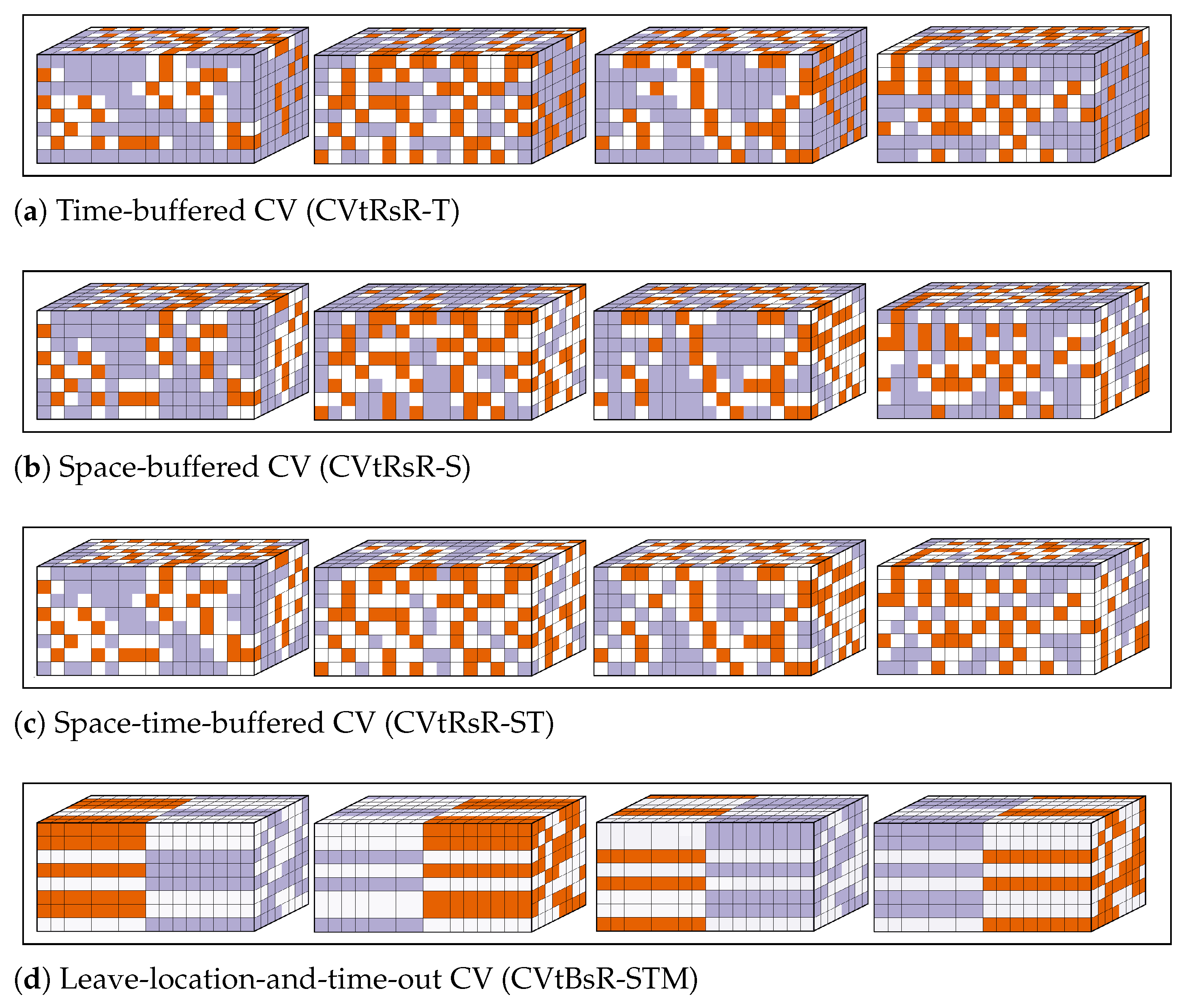
Recent work by Meyer et al. [11] highlights how, for spatiotemporal interpolation problems, the results of conventional CV differ from the results of what they call “target-oriented” CV (versions of CV that address each and/or both dimensions, namely, “leave-location-out”, “leave-time-out” and “leave-location-and-time-out”). The authors attributed the lower error estimated by conventional CV to spatiotemporal over-fitting of the models and propose a forward feature selection procedure to improve interpolation results.

The applicability of solutions that consider the temporal and/or spatial auto-correlation is worth exploring, but the optimal strategy will depend on the modeling goal. It is important to make the distinction, as previous works have, between interpolation and forecasting problems. Unlike previous work on spatiotemporal data, the focus of this study is on forecasting, meaning that the aim is to make predictions about the future/new locations. Even after that is established, it may still be the case that the best evaluation procedure when the goal is to make predictions about unseen locations might differ from the best strategy when the aim is to make predictions in known sites.

2. Materials and Methods

The different estimation procedures being compared are presented in Section 2.1. We investigate their performance on datasets of randomly-generated artificial spatiotemporal data, as they provide a foundation for better understanding the properties of the different estimation methods. We then evaluate their performance in the real-world case studies. All datasets used are presented in Section 2.2. Section 2.3 describes the experimental methodology that was used to compare the procedures. All code necessary for replication of these experiments is freely available at https://github.com/mrfoliveira/STEvaluation-MDPI2021 (accessed on 20 March 2021).

2.1. Estimation Procedures

The estimators tested in this paper include time-wise holdout methods (one-time, H; Monte Carlo, MC), Cross-Validation (CV) and prequential evaluation (P).

2.1.1. Time-wise Holdout Procedures

First, we illustrate the train/test allocation procedures for OOS procedures other than prequential evaluation. For time-wise holdout, one split-point in time is chosen so that all previous observations are used for training and subsequent cases are used for testing—this is usually chosen so that a certain proportion between training and testing is achieved (see Figure 1a). In the case of time-wise Monte Carlo, several data-split points are randomly generated, with a fixed size window of previous observations being used for training, and another fixed size window of future values being used for testing (see Figure 1b). The window sizes should be set in a way that not only takes into account the desired proportion between training and testing block size, but also guarantees that enough observations remain outside of the train/test blocks at each iteration to make the random generation of split-points meaningful.

2.1.2. Cross-Validation Procedures

Methods to assign observations into cross-validation folds that were tested in our experiments include: standard cross-validation, where instances are randomly assigned to folds (tRsR, see Figure 2a), ignoring both time- and space-dependency dimensions; time-sliced CV, where the spatial dimension is ignored and time-slices are assigned to folds randomly (tRsA, see Figure 2b); and spatial block CV (also referred to as “leave-location-out” CV), where the temporal dimension is ignored and spatial blocks are assigned to folds either randomly (tAsR, see Figure 2c), in contiguous blocks (tAsC, see Figure 2d) or in a systematic, checkered pattern (tAsS, see Figure 2e).

2.1.3. Block Cross-Validation and Prequential Evaluation Procedures

When time is divided into blocks, prequential evaluation can also be applied. In this scenario (tBsA; see Figure 3a and Figure 4a), also referred to as “leave-time-out” CV, fold assignment ignores the spatial dimension. If space is also divided into blocks, then different types of spatiotemporal CV can be achieved by having the spatial assignment of folds be either random (tBsR; see Figure 3b and Figure 4b), in contiguous blocks (tBsC; see Figure 3c and Figure 4c) or in a (systematic) checkered pattern (tBsS; see Figure 3d and Figure 4d).

Note that, in what we call prequential evaluation, temporal order is always respected even when dividing data into spatiotemporal blocks, i.e., if a block in space-time is used for testing, then only blocks with previous time-stamps are used for training. Whether the spatial region in the test set is included in the training set is optional (rmS indicates that spatiotemporal data from the past but in the spatial region of the test set are not used in training). Moreover, the number of previous blocks in time used for training can either increase at each blocked time step as in Figure 4 (growing window (grW)) or be fixed as in Figure 5a,b,d (sliding window (slW)). The idea of the sliding window approaches is to maintain some consistency in terms of the training size of the different repetitions, whilst the motivation for the growing window approaches is to take advantage of all past data for training the models. Which alternative is the best is highly domain dependent and may also be strongly related with phenomena such as concept drift where “forgetting” the older data may actually be beneficial for models.

2.1.4. Buffered Cross-Validation

Methods that remove a block of observations in the neighbourhood of the test set (in the temporal and/or spatial dimensions) from the training set have also been considered in our comparisons.

In the case of standard CV, for each instance in the test set, some past and future observations at that location are removed and/or observations within a certain distance from the location are removed (CV-T, CV-S or CV-ST; see Figure 6). This is akin to modified CV mentioned above in a time series context. The same process can be applied to spatiotemporal CV. In that scenario, if the buffer is set to the maximum distances between any two points in space/time (CV-STM; see Figure 6d), the result is what is sometimes called “leave-location-and-time-out” CV.

When time block CV is used, some previous and future observations are removed around the test set (CV-T). This is similar to $hv$-block CV. However, while $hv$-block CV is repeated for each instance of the whole set (therefore including overlapping test sets), the procedure is only repeated here for each non-overlapping block of sequential time.

In spatial random or contiguous block CV, a spatial buffer can be applied, so that locations within a pre-defined spatial distance of the test set are removed from the training set (CV-S). This is, again, similar to $hv$-block CV in space.

Table 1. Cross-validation and prequential evaluation fold assignment procedures.

		Time	Space
Cross-validation	Standard	random	random	tRsR $•†‡$
	Time-sliced		all	tRsA
	Spatial block	all	random block	tAsR •
	Checkered spatial block		systematic	tAsS
	Contiguous spatial block		contiguous	tAsC •
Cross-validation & Prequential evaluation	Time block	block	all	tBsA †
	Spatiotemporal block		random block	tBsR ‡
	Spatiotemporal checkered block		systematic	tBsS
	Spatiotemporal contiguous block		contiguous	tBsC

† Time-buffered CV variation included. • Space-buffered CV variation included. ‡ Space-time buffered CV variation included.

summarises the different train/test assignment procedures used for CV and prequential evaluation methods.

2.2. Datasets

As mentioned above, both artificially generated and real-world datasets were used for our comparative study.

2.2.1. Artificial Datasets

Artificial data were generated by stationary spatiotemporal autoregressive moving average (STARMA) models as proposed in [28] and implemented in R package starma [29].

The models are denoted by $STARMA(p_{{\lambda }_1{\lambda }_2\cdots {\lambda }_p},q_{m_1{m}_2{\cdots }_p})$ where p is the autoregressive order, q is the moving average order, ${\lambda }_l$ is the spatial order of the kth autoregressive term and $m_k$ is the spatial order of the kth moving average term. If $q=0$, then $STAR\left(p_{{\lambda }_1\cdots {\lambda }_p}\right)$ will suffice; if $p=0$, then it may be denoted by $STMA\left(q_{m_1{\cdots }_p}\right)$. Nonlinear versions of STAR models, $NLSTAR\left(p_{{\lambda }_1\cdots {\lambda }_p}\right)$, are generated by applying a nonlinear function at each autoregressive step (similar to what is done in [5] to obtain nonlinear AR models).

In datasets generated by a $STAR\left(2_{10}\right)$ model, a value measured at location i and time t is directly influenced by the values of location i and of its first-degree neighbours at time $t-1$ and by the values of location i at time $t-2$. Note that neighbours of lower order must be considered “closer” than neighbours of higher order (according to some metric of distance).

In this study, for each model of type STARMA (with $p=q$), STMA, STAR and NLSTAR, four sets of coefficients of each order $2_{10}$, $2_{01}$ and $2_{11}$ are generated randomly (within intervals likely to respect stationarity conditions) until the resulting STARMA models are stationary. In the case of NLSTAR, a nonlinear function is also randomly selected from a pre-defined set. Then, using grids of $10\times 10$ and $22\times 22$ equally spaced locations, data are generated with time series lengths of 250 and 400. However, after this step, the first 100 observations at each location are discarded in an effort to avoid dependence on initial conditions; outer locations are ignored so each used location has information for its four first order neighbours—top, bottom, left and right. Thus, 150 and 300 observations on $8\times 8$ and $20\times 20$ grids are kept for forecasting performance analysis. For details on the data generation process, consult Appendix A.

Spatiotemporal Embedding

To apply standard regression techniques to the spatiotemporal forecasting problem, the generated datasets have to be transformed in some way so each instance has a set of predictors. A simple way to do this is by spatiotemporal embedding, i.e., by using previous values measured at the given location and its neighbours as predictors. The order of spatiotemporal embedding can be denoted in the same way as the $STARMA$ order. All artificially generated datasets were embedded with order $3_{110}$. In total, 192 artificial datasets were generated using this embedding strategy.

2.2.2. Real-World Datasets

Seventeen variables from seven different real-world data sources were used as independent univariate datasets for experimental validation of the performance estimation procedures. The measured variables describe data from environmental monitoring contexts, from air pollution to climate and soil characteristics. A summary of the characteristics of each dataset can be found in

Table 2. Description of real-world datasets, including the total number of observations that are available, and the percentage of all possible combinations of location and time-stamp that they represent.

			Time		Locations		Total
Dataset	#	Variables	#IDs	Frequency	#IDs	Distribution	#	% Available	Source
MESA Air Pollution	1	NO${}_X$ concentration	280	bi-weekly	20	irregular	5.6k	100	[30] 1
NCDC Air Climate	2	precipitation, solar energy	105	monthly	72	irregular	7.6k	100	[30] 1
TCE Air Climate	3	ozone concentration, air temperature, wind speed	330 360 360	hourly	26	irregular	8.6–9.4k	100	[30] 1
COOK Agronomy Farm	3	water content, temperature, conductivity	729	daily	42	irregular	22–23k	73–74	[31,32] 2
SAC Air Climate	1	air temperature	144	monthly	900	regular	130k	100	[30] 1
RURAL airBase	1	PM10 concentration	4382	daily	70	irregular	149k	49	[33] 3
BEIJ Beijing UrbanAir 5	6	PM25, PM10 & NO${}_X$ concentration, air temperature, humidity	6.6k	hourly	36	irregular	152–163k	64–69	[34] 4

¹ Downloaded at: http://www.di.uniba.it/~appice/software/COSTK/index.htm, accessed on 12 March 2018; ² Loaded from R package GSIF version 0.5-5.1 (https://cran.r-project.org/web/packages/GSIF/index.html, accessed on 9 December 2020); ³ Loaded from R package spacetime version 1.2–3 (https://cran.r-project.org/web/packages/spacetime/index.html, accessed on 9 December 2020); ⁴ Downloaded at: https://www.microsoft.com/en-us/research/publication/u-air-when-urban-air-quality-inference-meets-big-data/, accessed on 18 October 2017; ⁵ Since there was more than one measurement for some hours, for this extension, we rounded the time-stamps to the closest hour and calculated the median values per hour and location (the original measurements are used in the conference version of the paper).

. The size of the datasets varies from small networks of 20 sensors to larger networks of 900 geolocations. The spatial distribution of locations from each data source can be seen in Figure 7. Although most sensor networks are irregularly distributed in space, one of them forms a regular grid of 0.5 × 0.5 degrees of longitude/latitude. The datasets also vary in terms of time series size (from 280 time points to over 6000) and sampling frequency (from hourly to monthly). About half of the variables were measured at every point in time and space, with no missing values. However, for others, only a percentage of location and time-stamp pairs (from 49% to 74%) have available values, due to, for instance, some sensors only being installed later in the measurement period.

Spatiotemporal Indicators

To compare performance, a learning approach had to be selected that would work with the different dataset characteristics. Unlike the artificial datasets, most real-world sensor networks are not distributed in a regular grid, so the simple spatiotemporal embedding used for the artificial datasets seemed over-simplistic. The approach adopted instead was the one proposed in [26], which relies on the definition of spatiotemporal distance in Equation (1), where the distance between two observations $y_i$ and $y_j$, measured at locations $l_i$ and $l_j$ and times $t_i$ and $t_j$, respectively, depends on the geographical distance between locations $l_i$ and $l_j$ and the temporal difference between time stamps $t_j$ and $t_i$.

$$dis{t}_{ST}(y_i,y_j)=d_S(l_i,l_j)\times \alpha +d_T(t_j,t_i)\times (1-\alpha )$$

(1)

For each observation, the following predictors were calculated and used:

• A temporal embed of values measured at the location: The temporal embed size was set to 7 meaning that, when predicting the target value at time t, we are using the values measured at times $t-1,t-2,\cdots ,t-7$ as predictors.
• Spatiotemporal indicators built by calculating summary statistics from the neighbouring observations within three dataset specific boundaries of spatiotemporal distance: We calculated the mean of target values measured in the past and within each spatiotemporal boundary, its standard deviation and a weighted mean inversely proportional to spatiotemporal distance of each measurement to the observation.
• Ratios between mean and weighted mean of values within spatiotemporal neighbourhoods of increasing radius: That is, if we consider three boundaries ${\beta }_1$, ${\beta }_2$ and ${\beta }_3$ of spatiotemporal distance such that ${\beta }_3>{\beta }_2>{\beta }_1$, then ratios are calculated between the mean target values within spatiotemporal distance ${\beta }_3$ and ${\beta }_2$, as well as ${\beta }_2$ and ${\beta }_1$.

When deciding on the value of $\alpha$ that weighs spatial and temporal distance and the maximum spatiotemporal distance $\beta$ defining the boundaries for each spatiotemporal neighbourhood, some consideration was taken so that most neighbourhoods would not be empty. We set the value of $\alpha$ to 0.25 for most datasets, and to 0.5 for datasets NCDC and SAC which have a number of unique locations that is more than half the number of different timestamps. Since the spatial distribution and sampling frequency varies greatly across datasets, we set the neighbourhood boundaries in proportion to the maximum spatial and temporal distances. That is, the distances between all locations and differences between all timestamps were calculated before any other processing or data splitting and normalised to be within $[0,1]$, so that we could choose the same $\beta$ values for all datasets. We used $\beta \in \{0.0250,0.0375,0.0500\}$. In a deployment setting, this would require knowledge of the desired prediction horizon in advance so that time differences could be normalised to $[0,1]$ properly. This may be reasonable in some scenarios such as the study at hand; alternatively, one could set an absolute rather than relative boundary.

Table 3. Parameter $\alpha$ and distances between stations (in kilometres) and spatial radius of each spatiotemporal neighbourhood when temporal distance is zero ($d_T=0$), $r_i={\beta }_i/\alpha$, $\beta \in \{0.0250,0.0375,0.0500\}$.

Data	$\mathit{\alpha }$	min. dist.	max. dist.	${\mathit{r}}_1$	${\mathit{r}}_2$	${\mathit{r}}_3$
MESApol	0.25	0.08	65.11	6.51	9.77	13.02
NCDC	0.5	1.43	4426.17	221.31	331.96	442.62
TCEQ	0.25	4.38	1214.35	121.43	182.15	242.87
COOK	0.25	0.06	0.90	0.09	0.14	0.18
SAC	0.5	31.40	2693.96	134.70	202.05	269.40
RURAL	0.25	3.80	814.53	81.45	122.18	162.91
BEIJ	0.25	1.62	128.28	12.83	19.24	25.66

shows the minimum and maximum distances between spatial neighbours for each dataset source, as well as the maximum spatial radius of each spatiotemporal neighbourhood when temporal distance, $d_T$, is zero. While observations at zero temporal distance from the target are not included in the calculation of spatiotemporal indicators (only past observations are used in the calculation), this still provides an idea of the spatial extent of the spatiotemporal neighbourhoods at their maximum spatial radius. Figure 8 shows the spatiotemporal neighbourhood at these spatial radiuses, given the combinations of $\alpha$ and $\beta$, for dataset Cook Agronomy Farm. Locations that are considered neighbours at zero temporal distance are connected by lines.

2.3. Experimental Design

In this section, we present the evaluation procedure used to assess the accuracy of errors estimated by the evaluation procedures detailed in Section 2.1. We also present the error metrics used in this study and the learning process applied to each training set to obtain a prediction model.

2.3.1. Error Estimation Assessment

For each dataset: (1) The data are divided into an in-set and out-set. This is performed time-wise, so that the out-set consists of a percentage of the most recent observations. (2) A regression model is trained on the in-set and tested on the out-set. The error of this model obtained on the out-set is considered to be the “gold standard” error that estimation methods should be able to approximate accurately. (3) Several error estimation methods (cross-validation, prequential and out-of-sample methods), applied exclusively on data from the in-set, are used to approximate the “gold standard” (see Figure 9). The differences between the “gold standard” error and the error estimated by each estimation methodology can be compared over all datasets and learning model pairs.

Train/Test Sizing

The in-set was set to be 80% of the time-points. When using cross-validation or prequential evaluation on the in-set, 16 folds were used for artificial data and 9 folds for real data. When using OOS procedures on the in-set, the splits are always made time-wise. For holdout, estimations were made with test sizes of 20% (same proportion as the out-set) and 6%/11% for artificial/real in-set data (the proportions used in the last block of time-block CV).

Note that the dataset is divided into the same number (16 or 9) of equally-sized folds across all variations of CV. In the interest of fairness, the test size of one variant of time-wise holdout was defined to correspond to the size of one fold in CV. All of these methodologies use the whole given in-set to make estimates. However, time-wise Monte Carlo estimations, by definition, use only a fraction of the dataset for each iteration—meaning the sizing of these competing procedures can never be made entirely “fair”. The option taken in our study was to keep the proportion between train and test sizes roughly the same as that used in CV, i.e., the percentages used for training and testing in Monte Carlo approximate the estimation on the last block of a 16-fold or 9-fold time block CV performed on subsets of the in-set. Thus, Monte Carlo estimations were averaged over 16 repetitions with training (testing) performed on 47% (3%) and 55% (4%) of the in-set for artificial data and averaged over 9 repetitions of training (testing) on 44% (6%) and 53% (7%) of real data. Buffer sizes are set to the highest embed size or spatiotemporal neighbourhood radius.

2.3.2. Error Metrics

The error of learning algorithms is measured by Normalized Mean Absolute Error (NMAE), defined by Equation (2). where $z_i$ is the observed value, $\widehat{z_i}$ is the prediction and $\overline{z}$ is the mean of Z in the test set. By opting for a normalised metric instead of the more widely used MAE, comparisons between error estimation methods across datasets can be made more easily.

$$NMAE=\frac{{\sum }_{i=0}^n|{\widehat{z}}_i-z_i|}{{\sum }_{i=0}^n|z_i-\overline{z}|}$$

(2)

2.3.3. Training Process

In this section, we explain how we handle missing data and present the learning models selected.

Missing Data

Some of the real-world datasets have missing data, either due to failures in data acquisition or due to sensors being set up at later times. This can cause data to be missing in the spatiotemporal indicators used as predictors as well, since they are calculated based on neighbouring values recorded in the past. After calculating the predictors and dividing the datasets into in-set and out-set (or training and test sets, within the in-set) but before any learning is carried out, all columns that have 20% or more of their data missing from the in-set (or training set) are discarded as they should not be very useful predictors, since imputing values based on less than 80% of observations could lead to bias in the model. The remaining missing data are dealt with as follows: first, any rows that have too many values missing (set at 20% of columns) are discarded from the training set; then, missing values for both the training and test sets are imputed as the median of that column in the training set. These thresholds were set at 20% in an attempt to strike a balance between minimisation of loss of information caused by discarding of observations and mitigation of bias introduced into the learning process due to possibly inaccurate imputed values.

Learning Models

The process is repeated over each dataset using four different learning algorithms: a linear regression model (LM) (R package stats [35]), a multivariate adaptive regression splines model (MARS) (R package earth [36]), a regression tree (RPART) (R package rpart [37]) and a random forest (RF) (R package ranger [38]).

3. Results

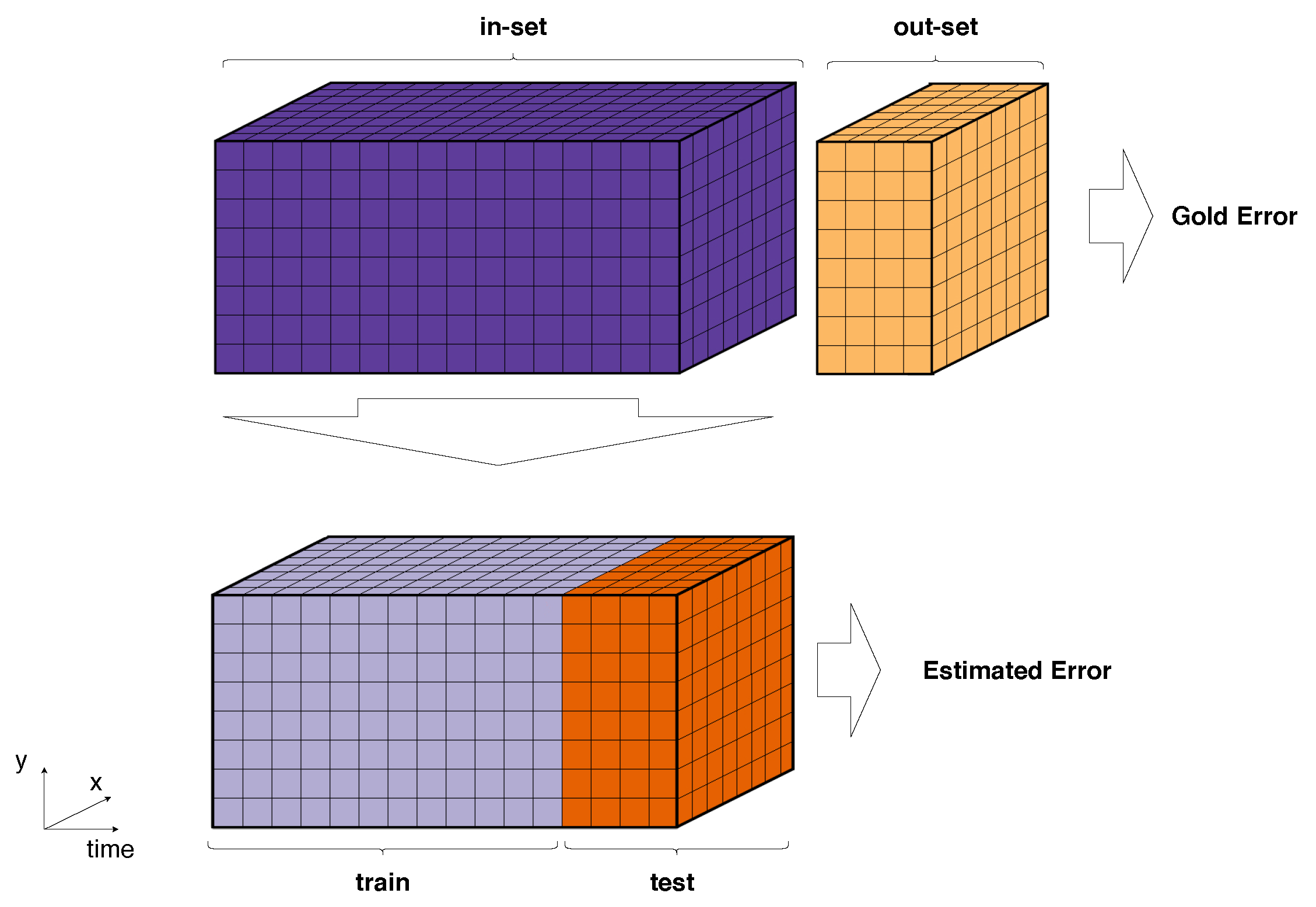
The estimation error is defined as the difference between the error estimated by a procedure using the in-set, $Est$, and the “gold standard” error incurred on the out-set, $Gold$, $Err=Est-Gold$. Note that experiments with methods that rely on non-random spatial blocking were not carried out using real-world datasets due to issues arising from irregular spatial distributions. Time-buffering without time-blocking in real-world scenarios caused issues related with buffer size/neighbourhood radius. Results for variations of prequential evaluation using sliding window and/or removing locations in the test set from the training set are not reported as they were consistently out-performed by their growing window counterparts (although the difference was not statistically significant).

3.1. Median Errors

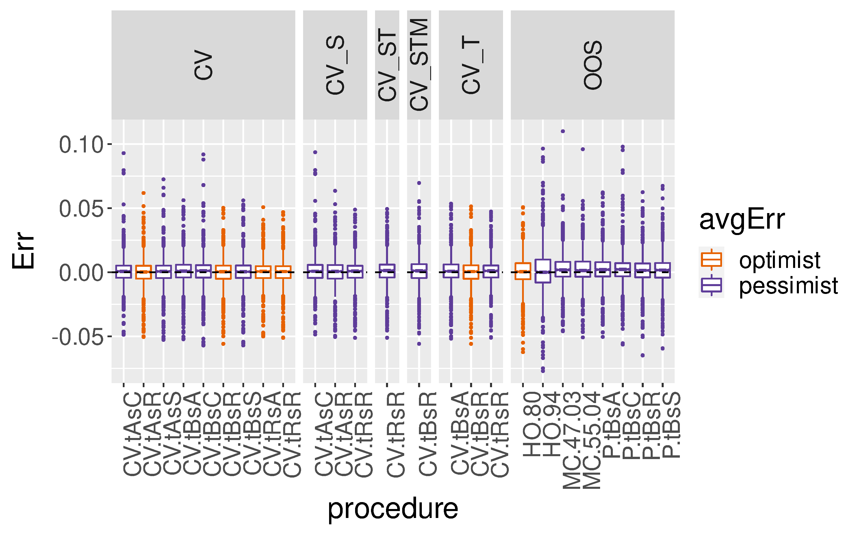
Figure 10 and Figure 11 show the distribution of estimation errors for artificial and real-world datasets. The sign of the error indicates whether the estimates (the median errors obtained across test sets for each dataset and learning model pair) produced by a procedure underestimate or overestimate the error. The box plots show the median errors incurred by each method, but the boxes are coloured according to the average error obtained by each method. A procedure that produces average errors below zero, underestimating error, is considered overly optimistic.

In Figure 10, all procedures appear centred around zero. However, three of the cross-validation procedures underestimate the median error, on average, even when using some form of block CV. This effect is usually mitigated when a type of buffering is applied (temporal, spatial or spatiotemporal). Most OOS procedures overestimate the error, on average, with the exception of holdout at 80%.

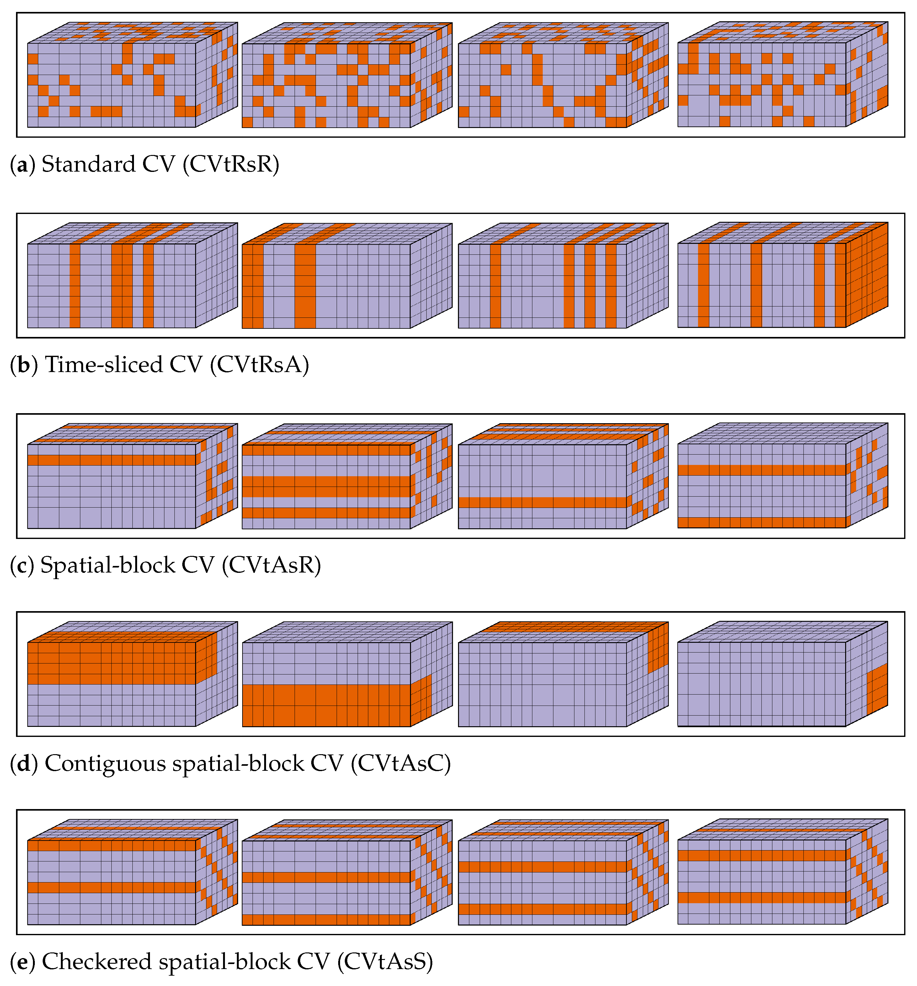
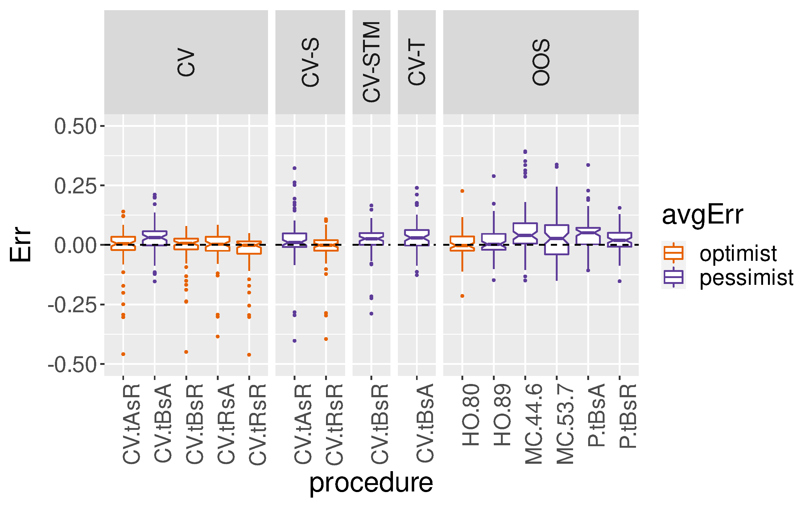
Figure 11 shows larger differences between procedures. Is is important to note that standard CV (CVtRsR) underestimates the error in over 55% of cases. We observe this problem even after applying a spatial buffer. Note that spatial-buffered CV estimates were not obtained for a fraction of real datasets due to problems associated with the irregularity of sensor network locations.

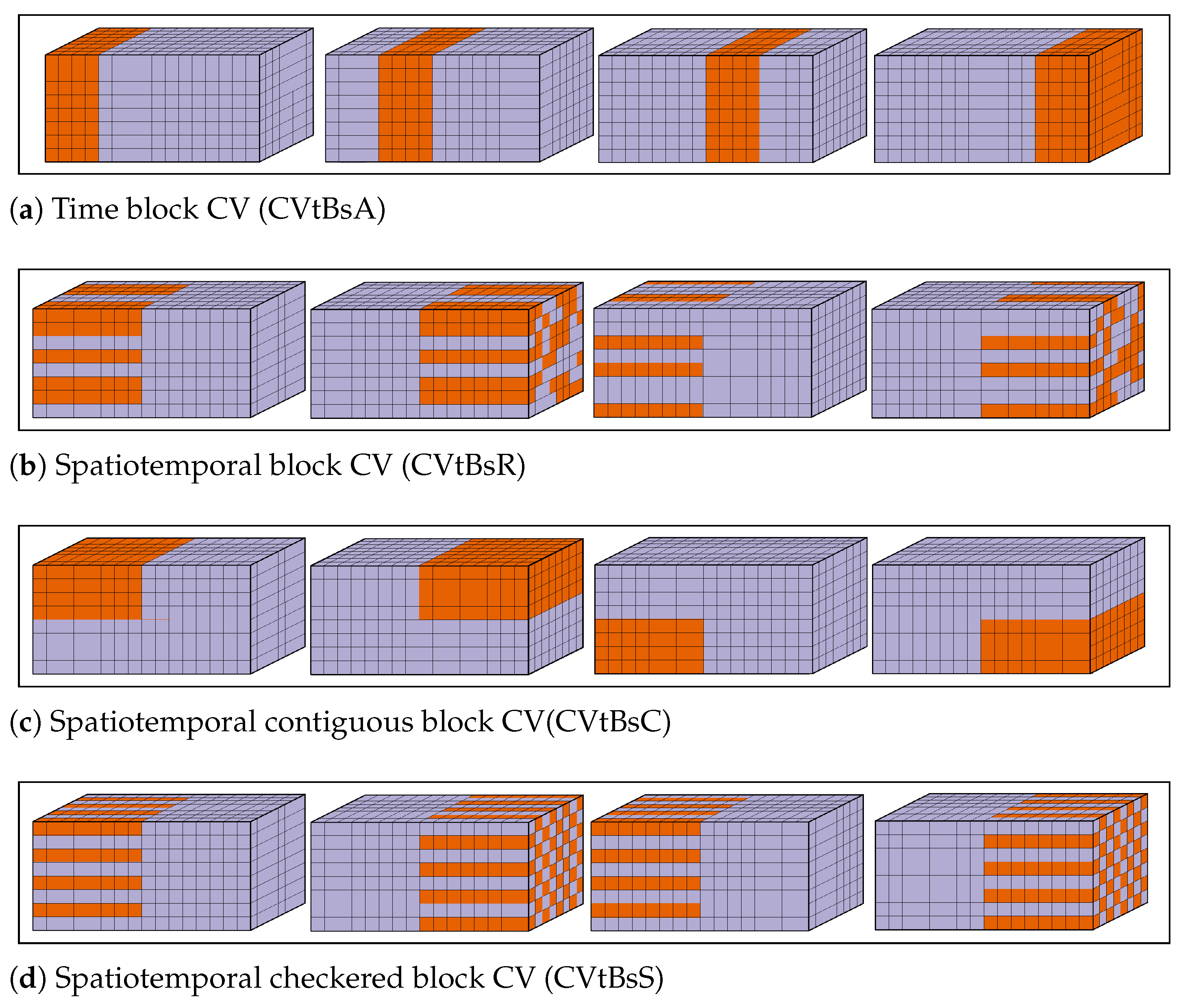
Spatial block CV (CVtAsR), time-sliced CV (CVtRsA) and spatiotemporal block CV (CVtBsR) are also overly optimistic, on average, in their error estimates. However, OOS procedures, temporal-block CV and other variations of block CV using buffers seem to be less prone to underestimate the error.

3.2. Relative Errors

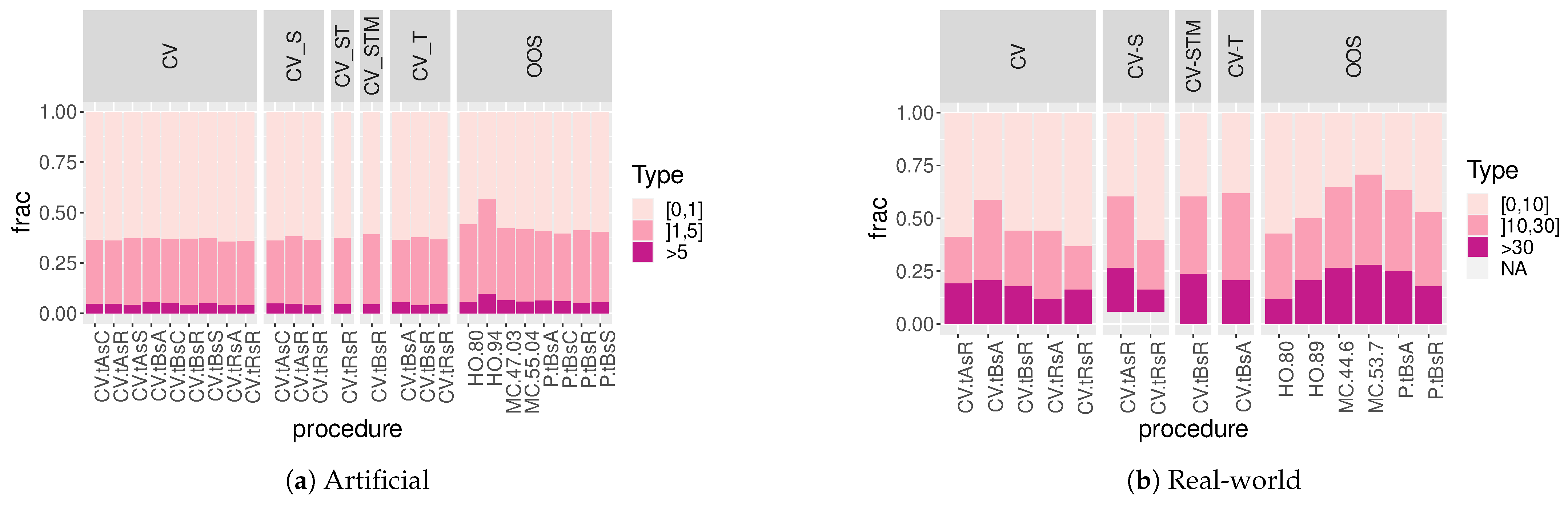
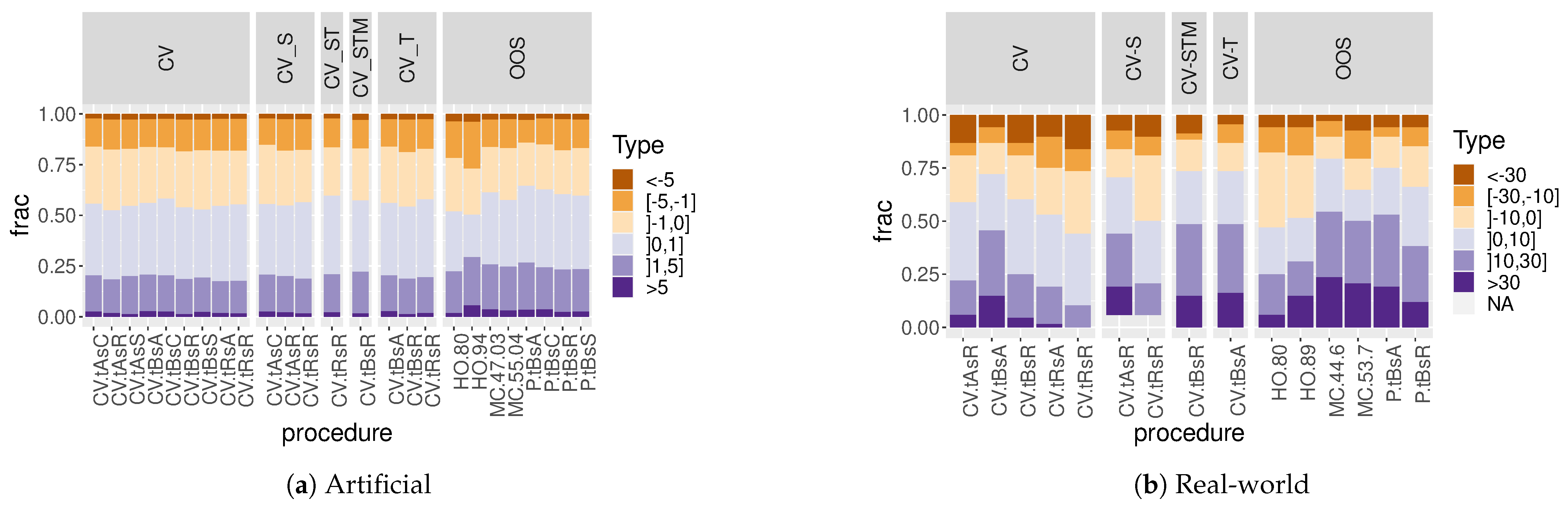
Other useful metrics to analyse are the relative absolute error as defined by $AbsRelErr=|Est-Gold|/Gold$ and the relative error as defined by $RelErr=(Est-Gold)/Gold$. Figure 12 and Figure 13 show the distribution of low, moderate and high errors and absolute errors. The binning is somewhat arbitrary but chosen so that comparisons might be useful.

In Figure 12a, we can see that all methods are quite accurate in their estimations: high relative absolute errors (defined as an estimated error that differs from the gold standard error by more than 5%) represent less than 10% of the results regardless of the method used, and almost all methods are able to estimate NMAE with low relative error (defined by not exceeding 1% of difference to the gold standard) in more than 50% of cases—the only exception being holdout ($H94.6$). Figure 13a breaks these errors down so optimistic errors can be distinguished from pessimistic errors. Although there are larger differences between methods when we consider the direction of the errors, they still behave quite similarly. However, as shown in the previous section, cross-validation methods tend to have a slightly higher proportion of optimistic estimations than most out-of-sample methods (except holdout).

In real-world scenarios (Figure 12b and Figure 13b), relative estimation errors are generally higher, and bins were chosen accordingly, so high relative absolute errors were defined as those that differ from the “gold standard” error by more than 30% instead of just 5% for artificial data. Even allowing for this higher tolerance for what may be considered a medium or small relative error, the evaluation procedures still show a higher proportion of high errors in these real-world scenarios than in the artificial datasets, with more than one method incurring in medium or high relative errors in more than half the cases. Here, MC procedures show the highest proportions of severe relative error, but some other methods are not far behind. If we take into account whether these errors tend to be overly optimistic or pessimistic, as in Figure 13b, we find even more contrast between different methods. It is clear in this figure that standard CV (CVtRsR), while avoiding higher overestimations of error, presents the highest fraction of highly optimistic errors, and the highest proportions of optimistic errors in general (closely followed by holdout). If using cross-validation methods, large proportions of highly optimistic errors are best avoided by blocking data in time (CVtBsA and CVtBsA_T) or using time slices (CVtRsA). However, using temporal block CV comes at the cost of larger proportions of highly pessimistic estimations, akin to the results obtained by using OOS methods other than 80/20 holdout.

3.3. Absolute Errors

Finally, we present results concerning the absolute errors incurred by estimation procedures, that is, $AbsErr=|Est-Gold|$. The mean ranks for artificial datasets can be found in

Table 4. Average ranks of absolute errors, calculated separately for cross-validation and out-of-sample procedures when estimating performance on 192 artificial datasets. The best results are in bold.

Type	Procedure	MARS	LM	RF	RPART	Overall
	CVtAsC	8.89	8.85	8.72	8.43	8.72
	CVtAsC_S	8.97	8.91	9.22	8.68	8.94
	CVtAsR	9.01	9.60	8.23	8.28	8.78
	CVtAsR_S	9.17	9.53	8.76	9.19	9.16
	CVtAsS	8.91	9.21	9.28	8.53	8.98
	CVtBsA	8.99	8.86	9.25	9.26	9.09
	CVtBsA_T	9.16	8.86	9.33	9.32	9.17
	CVtBsC	9.44	9.24	9.55	9.49	9.43
CV	CVtBsR	9.27	9.22	8.80	8.88	9.04
	CVtBsR_STM	9.98	9.28	9.74	9.55	9.64
	CVtBsR_T	9.30	9.28	8.86	9.22	9.16
	CVtBsS	9.12	8.84	8.72	8.92	8.90
	CVtRsA	8.08	8.47	8.51	8.57	8.41
	CVtRsR	8.33	8.66	7.82	8.62	8.36
	CVtRsR_S	8.80	8.73	8.43	9.26	8.80
	CVtRsR_ST	9.06	8.82	10.27	9.37	9.38
	CVtRsR_T	8.53	8.65	9.51	9.43	9.03
	HO80	4.48	4.52	4.39	4.74	4.54
	HO94	5.54	5.64	5.14	5.29	5.40
	MC4703	4.57	4.34	4.80	4.45	4.54
OOS	MC5504	4.54	4.56	4.43	4.41	4.49
	PtBsA_grW	4.36	4.18	4.43	4.14	4.28
	PtBsC_grW	4.28	4.27	4.51	4.41	4.37
	PtBsR_grW	4.18	4.31	4.19	4.15	4.21
	PtBsS_grW	4.05	4.18	4.11	4.41	4.19

. Although standard CV has the best average rank overall, the top performers for other models include spatial-block CV (CVtRsA), for MARS and LM, and time-slice CV (CVtAsR) when using RPART.

Time-slice CV ($CVtRsA$) and standard CV ($CVtRsR$) are two procedures that can be found within the top 5 average ranks for all four learning models. Within OOS procedures, spatiotemporal checkered-block prequential evaluation ($PtBsS$) is the only method that can be found within the top 3 average ranks for all learning models, and it also presents the best overall average rank.

Table 5. Average ranks of absolute errors, calculated separately for cross-validation and out-of-sample procedures when estimating performance on 17 real-world datasets. The best results are in bold.

Type	Procedure	MARS	LM	RF	RPART	Overall
	CVtAsR	4.47	4.47	5.47	5.06	4.87
	CVtAsR_S	5.71	5.24	4.76	4.88	5.15
	CVtBsA	5.65	6.12	4.53	6.29	5.65
	CVtBsA_T	6.00	6.41	4.82	5.88	5.78
CV	CVtBsR	4.88	4.82	4.59	4.82	4.78
	CVtBsR_STM	5.94	5.59	5.00	5.12	5.41
	CVtRsA	4.35	4.47	5.00	4.35	4.54
	CVtRsR	3.35	3.59	6.12	4.24	4.32
	CVtRsR_S	4.65	4.29	4.71	4.35	4.50
	HO.80	2.71	2.59	2.94	3.18	2.85
	HO.89	2.76	3.12	3.06	2.59	2.88
OOS	MC.44.6	4.12	4.06	3.65	4.00	3.96
	MC.53.7	4.59	4.47	4.18	4.35	4.40
	PtBsA	3.65	3.94	4.06	3.82	3.87
	PtBsR	3.18	2.82	3.12	3.06	3.04

shows average ranks for real-world datasets. Standard CV achieves the overall best rank. However, it does not rank within the top 5 best results when using RF. Only spatiotemporal block CV ($CVtBsR$) and space-buffered standard CV ($CVtRsR\_S$) are within the top 5 average rank of all learning models. The top 3 OOS procedures are consistently spatiotemporal block prequential evaluation ($PtBsR$) and holdout ($H80.20$ and $HO89.11$) across all learning methods, with $H80.20$ having the best overall average rank.

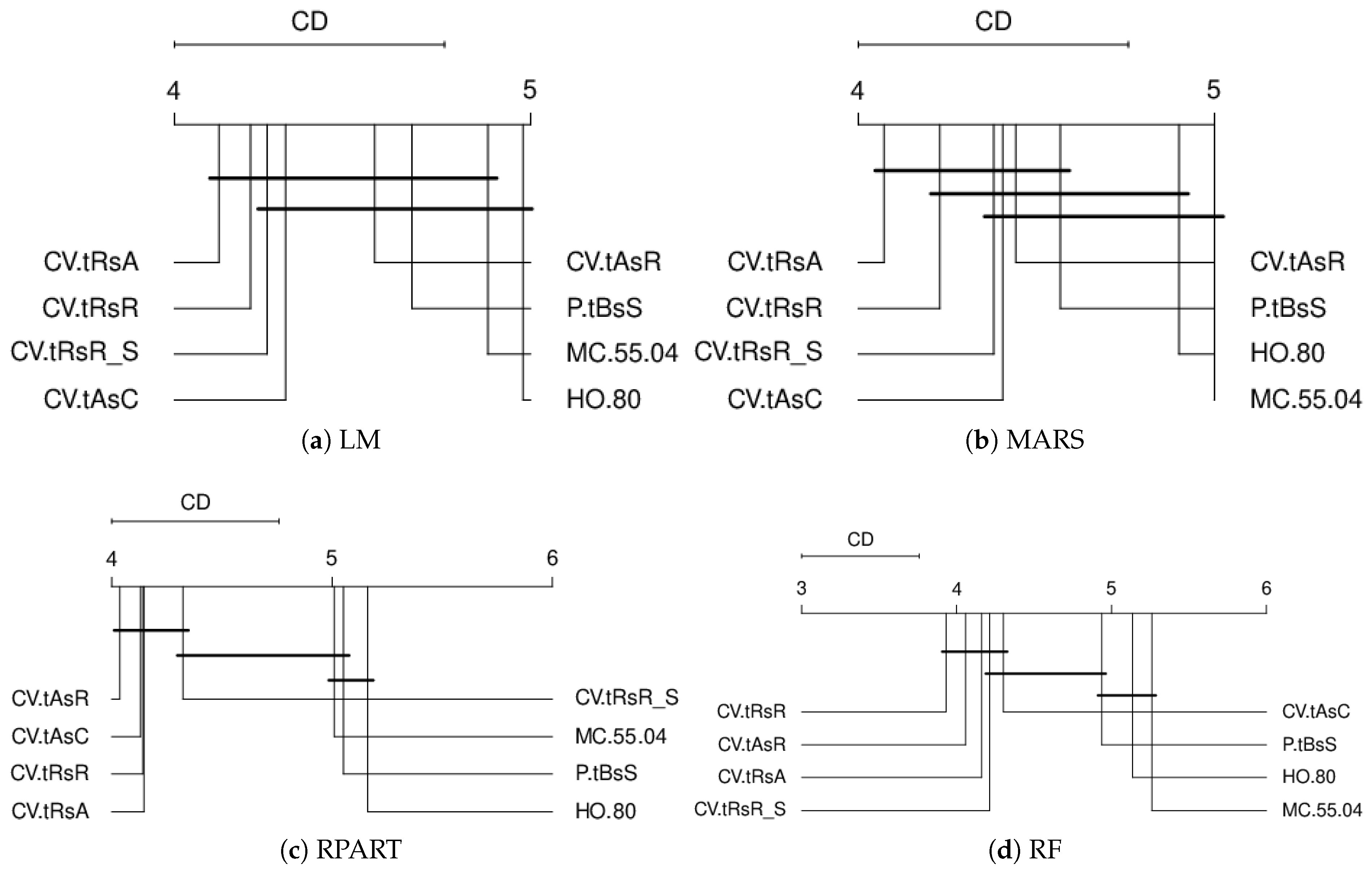
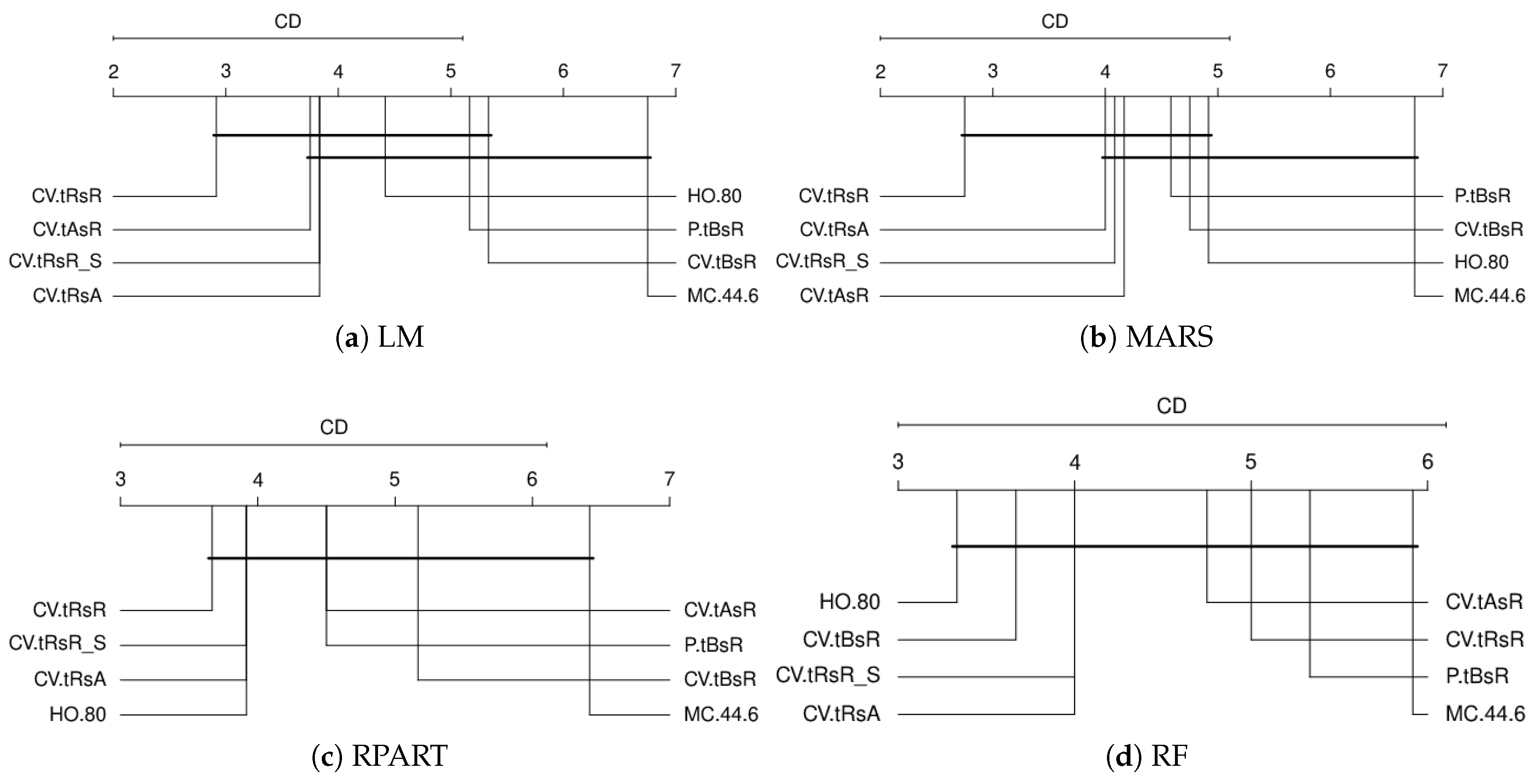
Statistical Significance

For statistical significance testing, we consider standard CV, 80/20 holdout, the top 5 CV methods with best overall average rank and the best OOS method of each type (holdout, Monte Carlo and prequential).

The Friedman–Nemenyi test is applied, with estimation procedures used as the “classifiers” or “treatments” (using R package scmamp [39]). Since there is an assumption that the datasets should be independent, separate Friedman tests are carried out for the results obtained by each learning model.

Figure 14 and Figure 15 show critical difference diagrams for the artificial datasets and all the real-world datasets. In the case of artificial datasets, we find significant differences between methods, indicating that most CV procedures significantly outperform some or all OOS methods in terms of absolute error, at 5% confidence level. For real-world datasets, no significant difference between estimation procedures is found at a 5% confidence level for tree-based models RF and RPART. However, a significant difference is found between standard CV and the selected Monte Carlo method when using LM and MARS.

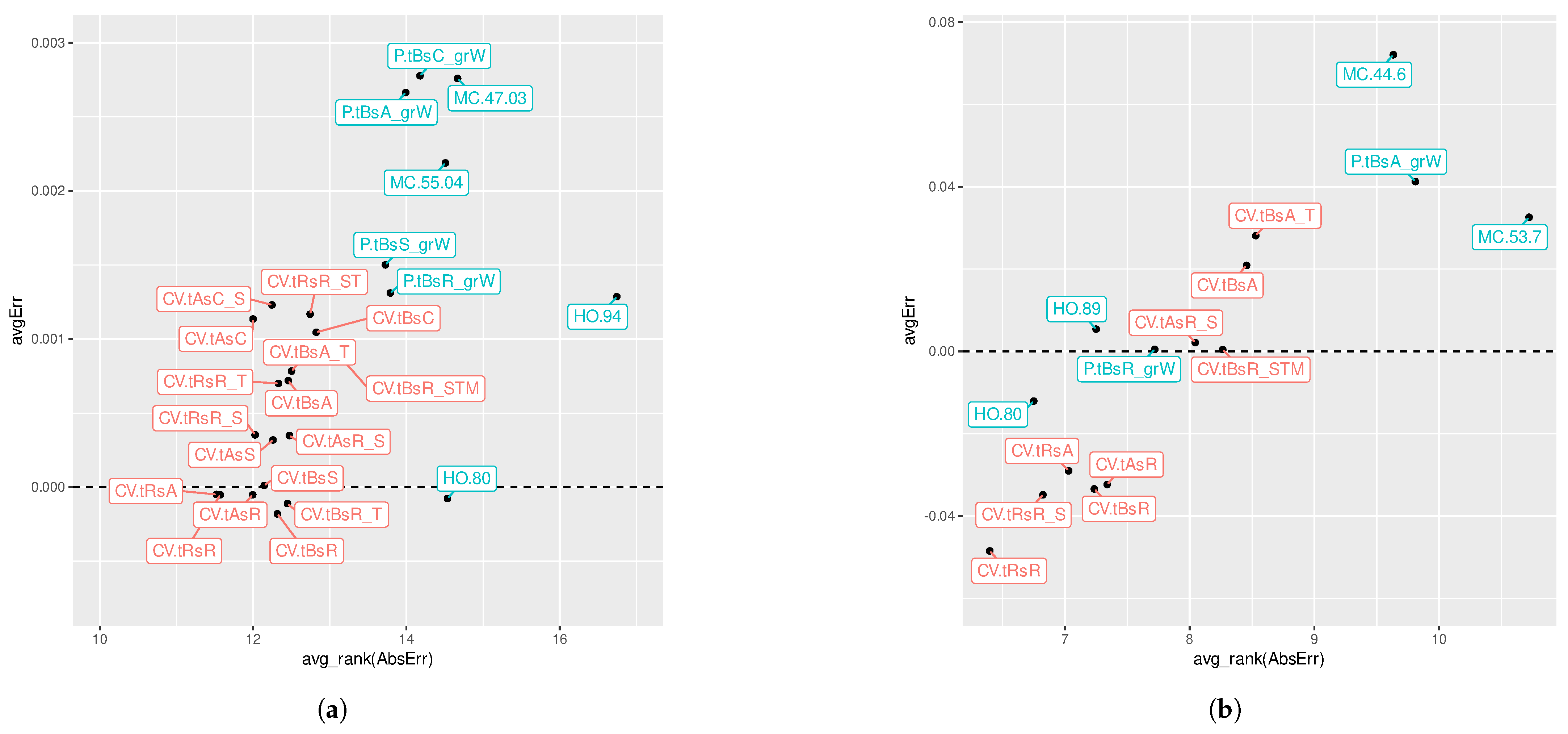
3.4. Median Errors vs. Average Rank of Absolute Errors

Having investigated the behaviour of median errors and the overall average ranks of absolute errors, we now compare them in Figure 16. Unlike Table 4 and Table 5, these average ranks are calculated including all methods against each other, instead of considering CV and OOS procedures separately.

It is clear from these figures that there is a trade-off where the most accurate estimators, that is, those with lower average ranks of absolute error (appearing towards the left side of the graphs) seem to also be severely over-optimistic in some of their estimates, with average errors below the dashed line indicating error underestimation.

This grows starker in the case of real-world scenarios, where methods are more spread-out across both the x- and y-axis, with many methods being diametrically opposed in relation to the dashed line, that is, there are methods suffering similar degrees of severe error underestimation as severe error overestimation. For example, standard CV ($CVtRsR$) has an average error that is a bit further below the dashed line than $PtBsA$ is above it; on average, they underestimate and overestimate errors, respectively, to a similar degree. Nevertheless, standard CV presents a better average rank in terms of absolute error. Moreover, standard CV is more optimistic, on average, than almost all other methods are pessimistic—the only exception being $MC.44.6$. In contrast, in the case of artificial data, even the most optimistic methods (such as standard CV) do not reach levels of underestimation as high as the overestimation incurred by more pessimistic methods.

Whether data are artificially generated or observed in the real-world, most prequential methods (those with blue labels) appear above the dashed line, indicating more pessimistic estimates—the only exception being 80/20 holdout which tends to be optimistic. Out-of-sample procedures are also mostly found from the middle to the rightmost side of the graphs, with higher average ranks indicating that they tend to be less accurate in their estimates than other methods when applied to the same scenario (i.e., the same dataset and learning model). In real-world cases, spatiotemporal block prequential evaluation ($P.tBsR$) stands out, since it manages to provide estimates that are quite accurate (very close to the dashed line), without being optimistic (on average) and not compromising as much in terms of absolute error rank (the method sits, on average, 1.32 positions below standard CV which achieved the best overall rank).

4. Discussion

In this paper, we provide an extensive empirical study of performance estimation for forecasting problems using both artificially generated and real-world spatiotemporal datasets. Previous empirical studies have already shown that dependence between observations negatively impacts performance estimation using standard error estimation methods such as cross-validation for time series [5,12,13], time-ordered Twitter data [14], spatial and phylogenetic data [15] and spatiotemporal interpolation [11].

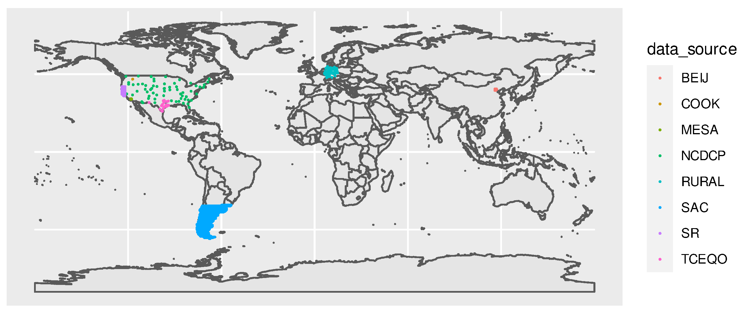
In this study, we first observe that error estimates are usually reasonably accurate, although estimations are much closer to the gold standard error in artificially generated data. Possible explanations for the lower relative errors found for artificial datasets, when compared to the real-world datasets, include the fact that: (a) some of the real datasets include missing data; (b) in the artificial datasets, locations were simulated on a regular grid, while only one of the real-world datasets had regularly distributed sensor stations; and (c) the underlying data generation process of artificial datasets was stationary and homogeneous, while real-world datasets may include drift of concept and/or contain heterogeneities.

Standard CV does raise problems when applied in the spatiotemporal context: while it often achieved the best average rank in terms of absolute error, it tends towards underestimation of errors and exhibits a considerable number of outliers of severe error underestimation. The issues with standard CV can be mitigated by taking into account the spatial and temporal dimensions in the fold allocation process and/or through the introduction of buffers. Indeed, for artificial datasets, contiguous-block spatial CV (CVtAsC) is one of the best in terms of approximating the “gold standard” error while also avoiding being overly optimistic in its estimates. For real-world datasets, adding a spatial buffer to spatially blocked CV (CVtAsR_S) not only approximates the error better than many other methods, but, on average, it also avoids being overly optimistic about errors. Temporal block CV (CVtBsA) also mostly avoids severe error underestimation, but that comes at a higher cost in terms of absolute error.

Holdout, similar to standard CV, presents much larger proportions of optimistic error estimations than other OOS procedures. In contrast, other out-of-sample procedures manage to much more often avoid being overly optimistic about errors; however, most of these methods did not, in general, do as well in terms of absolute difference to the “gold standard”, being less accurate in their estimates. The fact that OOS methods are less prone to underestimation of error might still be seen as an advantage over holdout and most other types of cross-validation. If so, these results could point to the temporal dimension being more important to respect when evaluating spatiotemporal forecasting methods. That considering the temporal dimension provides advantages in performance estimation is in line with previous research on time-ordered data [5,14].

There is a trade-off between the ability of methods to obtain better average ranks of absolute difference to the “gold standard” error and the avoidance of severe underestimations of error—depending on the application, one of these criteria may be considered more important than the other.

The evaluation procedures estimate performance by: (1) allocating observations to training and test sets; (2) constructing a number of models; and (3) computing statistics. Step (1) may require computing spatial and/or temporal distances, which might be quadratic on the number of observations. However, most resources will usually be spent learning on Step (2). The simplest approach, holdout, uses two partitions to construct one single model. The cross-validation approach will take an user-defined k partitions and construct k models on $(k-1)/k$ fractions of the training data. Temporal-block prequential models also use k partitions but construct $k-1$ models using an average of $(k-1)(k-2)/2$ partitions if using a growing window or a fixed number of at least one partition if using a sliding approach. The Monte Carlo model can be seen as running k holdouts, although learning from a smaller fraction of the total number of examples. Assuming that learning time tends to grow with dataset size, we would expect cross-validation to be the most expensive estimation procedure, followed by prequential evaluation with growing window. In practice, we often use parallelism to diminish execution time at the cost of spending more processing and memory resources.

Decisions around training and test set size also raise some questions about what is fair when comparing methods that utilise data in such a different way. Is it more important to maintain train or test set size consistent across methods? Should we focus instead on keeping the ratio between training and testing set size equal across procedures or the total number of test sets regardless of how data are divided? When comparing, for example, temporal-block CV with spatiotemporal-block CV, is it more fair if each of them uses the same number of temporal blocks (meaning that spatiotemporal block CV would have a higher number of folds overall) or would it be better if both methods use the same number of folds in total? The answers to these questions are not straightforward. We divided the datasets for cross-validation and prequential evaluation procedures into the same number of folds, which means that cross-validation methods had access to, at least, one more test set than their prequential counterparts; when translating this to OOS procedures, we decided to try to keep the ratio between test set and training set stable, which meant that Monte Carlo methods had access to smaller portions of the dataset in both training and testing phases. This is only one way of approaching this problem, but other options could also be valid. In fact, this experimental design can put Monte Carlo procedures at a disadvantage due to using smaller fractions of the in-set for error estimation—one possible explanation for the under-performance of Monte Carlo estimation methods, which have previously shown to fare well in time-series contexts [13]. Further exploration of the effects of in-set/out-set ratio, as well as training and test set sizes and number of partitions or Monte Carlo repetitions, may provide some insights into these questions. Buffer sizes were also fixed at only one value, that could be less than ideal. Further research could provide more insight into the effects of buffer size.

There are some other limitations to this work. For example, there is some bias in the experimental design which may affect the conclusions (e.g., it is reasonable to assume that holdout benefits, at least in terms of absolute error, from being the method used to set the “gold standard” error). The artificial datasets do not include non-stationarities or missing data, and the number of real-world datasets used is perhaps not large enough to make generalisations that would hold for all real-world spatiotemporal datasets, regardless of their characteristics. In addition, the spatiotemporal indicators that were used as predictors may also have an impact on the results.

Moreover, it should be noted that the results presented here for cross-validation and out-of-sample strategies differ in some respects from those reported in the conference version of this paper, which could be caused by several factors: (a) some differences and improvements in dataset generation and pre-processing; (b) an additional number of artificial datasets generated; (c) the inclusion of two additional learning models in the study; and (d) changes to the underlying random number generator in more recent versions of the R language used to implement our experiments. Even within this study, there are differences in the top performers, depending on the learning model used, as well as the types of dataset (real or artificial). Furthermore, when using the same datasets and model, some of the differences between procedures are not statistically significant.

Given all of this, it is difficult to make a definitive recommendation about which specific evaluation procedure should be the gold standard in spatiotemporal forecasting. However, our results add validity to the notion that the spatial and, especially, the temporal dimension should not be ignored when estimating performance in spatiotemporal forecasting problems, and some of the issues mentioned above could be addressed in future work.

Other directions of interest for future work would be: (a) setting the “gold standard” as forecasting future observations in new locations (instead of time-wise holdout); (b) controlling for the effect of including outer locations and/or introducing missing data in artificial data; and (c) designing solutions for contiguous assignment of spatial blocks, possibly using quadtrees, in the case of real-world (or artificial) datasets with irregular grids.

5. Conclusions

The problem of how to properly evaluate spatiotemporal forecasting methods is still an open one. Temporal, spatial and spatiotemporal dependence between observations negatively impacts performance estimation by standard error estimation methods such as cross-validation.

This work provides an extensive empirical study of performance estimation for forecasting problems using four different learning models and both artificially generated and real-world spatiotemporal datasets.

Our results show that, while standard cross-validation is, on average, a good estimator in terms of absolute error in relation to a “gold standard” error, it has issues with severe underestimation of errors in the spatiotemporal setting.

We recommend that methods that take into account the spatial and/or temporal dimensions of the problem be preferred over standard CV or holdout, which also seems to suffer from overly optimistic estimates. For example, space-buffered spatial block cross-validation approximates the error well and still makes use of all the available dataset, while more successfully avoiding being overly optimistic about errors. Out-of-sample procedures such as spatiotemporal block prequential evaluation also provide adequate estimates and have the advantage of avoiding situations where data are trained on future and tested on past data.