Data-Driven Leak Localization in Urban Water Distribution Networks Using Big Data for Random Forest Classifier

Abstract

In the present paper, a Random Forest classifier is used to detect leak locations on two different sized water distribution networks with sparse sensor placement. A great number of leak scenarios were simulated with Monte Carlo determined leak parameters (leak location and emitter coefficient). In order to account for demand variations that occur on a daily basis and to obtain a larger dataset, scenarios were simulated with random base demand increments or reductions for each network node. Classifier accuracy was assessed for different sensor layouts and numbers of sensors. Multiple prediction models were constructed for differently sized leakage and demand range variations in order to investigate model accuracy under various conditions. Results indicate that the prediction model provides the greatest accuracy for the largest leaks, with the smallest variation in base demand (62% accuracy for greater- and 82% for smaller-sized networks, for the largest considered leak size and a base demand variation of $\pm 2.5\%$). However, even for small leaks and the greatest base demand variations, the prediction model provided considerable accuracy, especially when localizing the sources of leaks when the true leak node and neighbor nodes were considered (for a smaller-sized network and a base demand of variation $\pm 20\%$ the model accuracy increased from 44% to 89% when top five nodes with greatest probability were considered, and for a greater-sized network with a base demand variation of $\pm 10\%$ the accuracy increased from 36% to 77%).

1. Introduction

Leakages in water distribution networks can cause great cumulative losses as small leakages can remain undetected for long periods of time. Direct losses are typically followed by the overall reduction of the functionality of the water distribution network, which usually manifests as a pressure drop on the user end. Moreover, leakages can potentially cause health hazards since microbiological contamination can enter the water distribution network and reach end users. Porous soil introduces additional difficulties, as even greater leakages can remain undetected since water is absorbed in the soil, and there is no evidence of the leakage on the surface. Thus, different technologies and methodologies have been proposed for leakage detection and localization. In a work by Jacobsz and Jahnke [1], leak detection using discrete fiber optic sensing was investigated. In a recent study by Nkemeni et al. [2], a wireless sensor network application was investigated, where processing for leak detection is performed at the sensor nodes. In a work by Wu et al. [3], a two-stage method was proposed, which first detects outliers from flow measurements using a clustering algorithm and then detects whether burst occurred. In the work of Rajeswaran et al. [4], a multi-stage graph partitioning algorithm was presented, which uses flow measurements to indicate a minimum number of additional measuring locations needed to narrow down leak location in large-size networks. In the work by Cody et al. [5], a linear prediction signal processing technique was used to extract features from acoustic data, which can detect and localize pipe leaks. In a work by Bohorquez et al. [6], an artificial neural network was applied to detect leak size and location in a single water pipeline.

Problems with leak detection and localization in pipelines that are used for transportation of hydrocarbon fluids are also extensively explored, since leaks can cause serious damage to people and the environment due to often hazardous fluid that is transported. A number of investigations were conducted, including a data-driven approach using the Kantorovich distance [7], feature extraction from acoustic signals [8], application of a least squares twin support vector machine [9], and a multi-layer perceptron neural network (MLPNN) [10]. A detailed overview of leak detection technologies in pipelines can be found in a review paper by Adegboye et al. [11].

Additionally, a number of studies considered strategies for optimal sensor placement since it greatly influences leak detection and localization methods efficiency. The optimization approach is most widely used, and thus different enhancements were considered, such as a clustering process prior to optimization [12], hybrid feature selection method [13], methods that reduce the optimization search space [14], and an investigation of the influence of measurement uncertainty [15]. A detailed overview of leakage detection methodologies can be found in review papers by Wu and Liu [16], Chan et al. [17], and Zaman et al. [18].

Software-based leakage detection methods can be divided into transient-based, model-based, and data-driven approaches. The transient-based approach is based on various analyses of pressure signals; the model-based approach analyzes residuals, i.e., compares pressure measurements with the pressure estimation based on a hydraulic network model; and the data-driven approach relies on collected data and mathematical operations in order to determine anomalies in pressure. In recent years, machine learning methods have been increasingly used for leakage detection and localization. Zhou et al. [19] and Pérez-Pérez et al. [20] investigated leak detection in a single pipeline. In the Zhou et al. [19]’s work, a convolutional neural network (CNN) was used to pinpoint leak locations in a 1500 m long pipe segment for different leak sizes, where the better prediction was obtained for greater leakages. Pérez-Pérez et al. [20] used a combined artificial neural network (ANN), where the ANN is first used to estimate the friction factor of the pipe and then to localize leak location. Tests were conducted for a 64.48 m pipe, for which it was reported that an average percentage error of 0.47% was achieved. Mounce et al. [21] proposed a system using an artificial neural network for online detection of bursts in water distribution networks that was shown to have 44% of alarms when burst really occurred, 32% of alarms in cases of unusual short-term increased demand, 9% of alarms due to industrial events and only 15% were false alarms, indicating the applicability of the proposed method. In the work of Jensen et al. [22], a sensitivity analysis of pressure residuals was performed to isolate possible leakage locations. The proposed methodology was applied to the actual water distribution network, where only a few false alarms occurred, and frequent alarms occured during the leakage. It was observed that the proposed methodology can isolate a limited set of candidate nodes, where better performance was observed for greater flows in the system. In the work of Zhang et al. [23], a data-driven and model-based approach was utilized, where large-scale water distribution networks were divided into leakage zones that were categories for multi-class support vector machine prediction. Large-scale networks were divided into up to 25 zones, with a classification accuracy of above 90% for a division into 25 zones, which further increased with smaller divisions into leakage zones. However, it must be taken into consideration that further leak localization needs to be conducted after the leak zone is determined to provide the exact leak location. Soldevila et al. [24] used a mixed model-based and data-driven approach in which the K-nearest neighbors (k-NN) algorithm is used to localize leaks. The proposed methodology was applied to three different sized networks, with leak, demand, and sensor measurement uncertainties. For the Hanoi benchmark network, for all considered uncertainties in the study, an accuracy greater than 90% was reported for the time horizon of one day using pressure sensor measurements from two sensors. Additionally, some network nodes were grouped since leaks from those nodes cannot be distinguished due to similar pressure measurements. Further study was presented by Soldevila et al. [25], where Bayesian classifiers were applied and greater accuracy than when using a k-NN approach was obtained. Both proposed methods were successfully applied to real water distribution network case studies where leak locations detected by the proposed methods were in the vicinity of the real leak locations. In the work of Quinones-Grueiro et al. [26], an unsupervised approach to leak detection was conducted for the Hanoi distribution network using three pressure sensors, where the average reported classification accuracy was 85% for leak magnitudes smaller than 2.5% of the total demand of the network for leaks detected within a time interval of one day. In the work of Zhou et al. [27], after the burst was detected, additional pressure sensors were placed at optimal locations and deep learning was employed to identify burst locations. The proposed methodology was applied to 58 synthetic burst cases, where in 57 cases the top five most probable pipes were correctly identified, and in 37 cases the top pipe was correctly located. However, it must be noted that the requirement for additional measurements can extend reaction time in case of a pipe burst. In the work of Sun et al. [28], a classification approach was utilized where pressure measurements in network nodes with no pressure sensors were estimated using the Kriging method. The Hanoi water distribution network was considered with a wide range of sensors, and it was reported that in the average case 70% accuracy was achieved; however, for some sensor layouts the reported accuracy was below 20%, which is believed to be due to the Kriging interpolation error. Javadiha et al. [29] used a convolutional neural network with pressure measurements for the Hanoi network, where for a one day time horizon the model accuracy varied from 56% for four sensors to 94% for 12 sensors considering leak size uncertainty, sensor noise, and base demand uncertainty. The Kriging method was also used in work by Soldevila et al. [30] with satisfactory leak localization in a real water distribution network case; however, when compared with their previous work, the Kriging method did not provide better results.

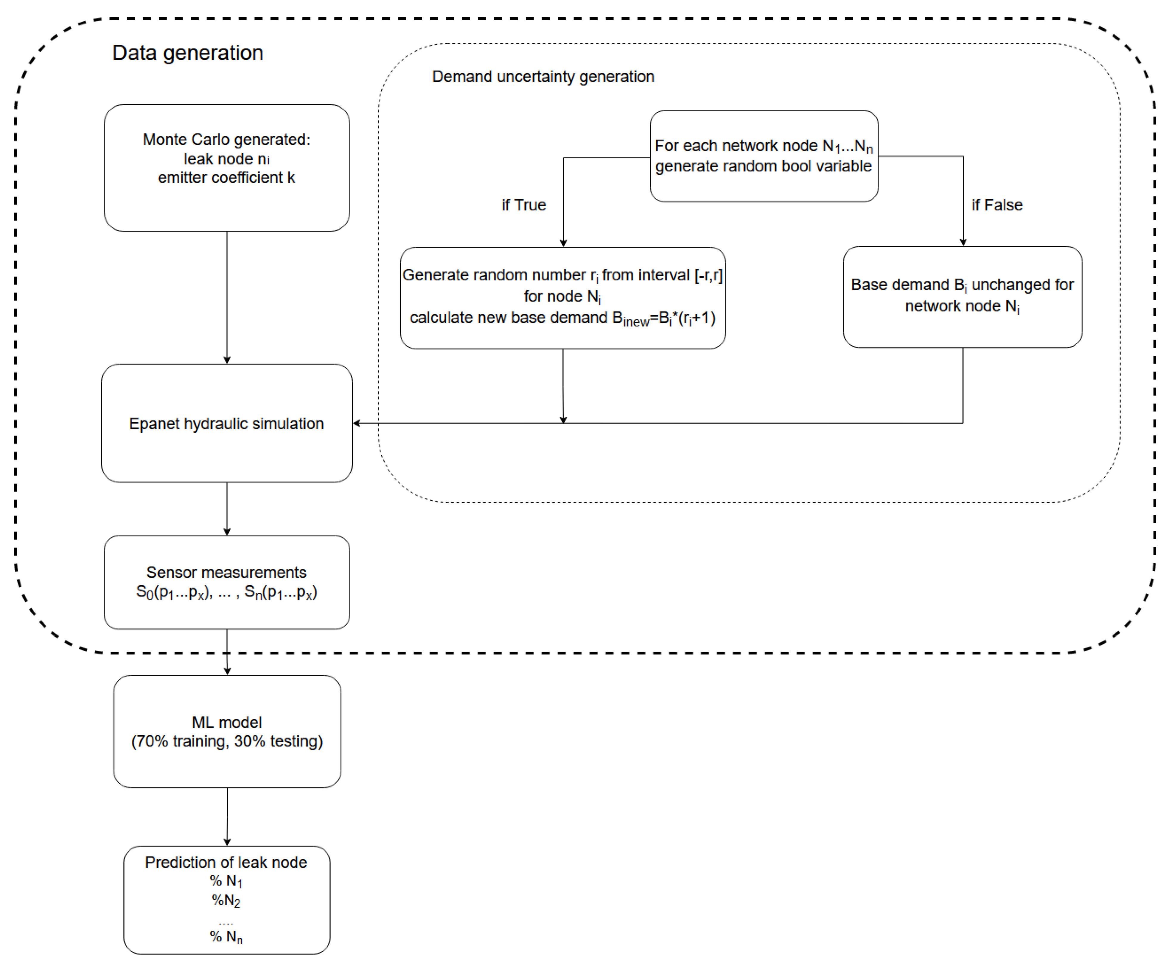
The main drawback of the machine learning approach is that only a small amount of real data measurements can be obtained for leak events. Additionally, when a new installation is made in the water distribution network, all previous records are not valid, consequently reducing the number of inputs for the prediction model. This is a common problem in rapidly developing urban areas. Thus, in this paper, a machine learning approach is presented, in which a great number of leak scenarios for randomly chosen network nodes and with different leak sizes under different demand conditions were conducted, to obtain a database of pressure sensor measurements that are inputs for the prediction model. This idea is similar to that proposed by Grbčić et al. [31] and Lučin et al. [32], where a number of Monte Carlo simulations were conducted to obtain a large number of inputs for a machine learning prediction model that successfully detects the location of contamination source and determines the number of contamination sources. To the authors’ knowledge, the currently proposed methodology has not been previously applied to the leak localization problem to obtain a large amount of synthetic data.

Model-based methods’ accuracy is greatly dependent on model calibration, where model uncertainties can decrease the method’s efficiency. In this work, model uncertainties are taken into consideration by including randomness for leak and demand values, so as to describe as many possible combinations of different leak scenarios. Machine learning classification is then utilized to detect the most appropriate leak scenario, which will be utilized to determine leak location. A random forest classifier was tested for leak localization on two different sized benchmark networks. Investigation of the influence of sensor layout and number of sensors on model accuracy was conducted. Different prediction models were constructed for different sizes of leaks and for different ranges of demand uncertainty to estimate model accuracy. This approach allows for a large number of varying measurements to be simulated in a short amount of time, thus providing relatively quick localization, which is suitable for use in real conditions. Additional model uncertainties such as pipe diameters, node elevations, etc. can easily be incorporated into the presented methodology.

The rest of the paper is organized as follows. In Section 2, the problem statement is defined with a description of the used benchmark water distribution networks and a description of the proposed methodology using a random forest classifier. In Section 3, results are presented for both benchmark networks investigating the influence of a different number of prediction model inputs and features, of different ranges of demand uncertainties and leak sizes, and of sensor layout on model accuracy. Additionally, an example of the application of the prediction model is presented. In Section 4, the main observations regarding the obtained results are presented with proposed further research. In Section 5, final remarks are presented.

2. Materials and Methods

2.1. Problem Statement

Model-based leakage detection methods rely on residuals obtained as a difference between measured and expected results from the simulation of a calibrated water distribution network model. Unfortunately, water distribution models used for simulation typically have estimated nodal demands, which greatly influences the accuracy of residual values, hence resulting in modeling errors that are the main drawback of this approach. Additionally, if sensitivity analysis is used with nominal leak values, further uncertainties are introduced. The basic premise of the currently proposed methodology is that the prediction model can be constructed from a large database of simulated measurement data, which should describe a variety of possible leak scenarios. Consequently, if a considerable amount of data is generated, with a set range of considered uncertainties, it is reasonable to assume that the real measurements can be determined from simulated events with randomly chosen leak parameters by the prediction model.

Leak scenarios were simulated using EPANET2 version 2.0.12. [33]. Simulation results were obtained with randomly chosen leak locations, leak size, and random demands of end users. Basic assumptions used in this work are that leaks can occur only in network nodes and that a single leak is present in the water distribution network. Sensor measurements are considered ideal. The used water distribution network models were considered to be calibrated, i.e., pipe diameter and roughness were considered to be known and well-calibrated. However, these uncertainties can easily be incorporated into the data generation stage and further investigation of these uncertainties is to be evaluated in future work.

The prediction model was constructed using raw pressure sensor measurements obtained every 15 min for a period of 24 h where different ranges of base demand variation were investigated. Although in a real case scenario base demands vary greatly on daily basis, several prediction models can be created with characteristic demand patterns, e.g., one for summer weekdays, one for winter weekends, etc. Additionally, a prediction model can be created specifically for night scenarios where smaller demand variations occur. This methodology is already used for leak detection when differences in flows are measured during the night to detect if the leak is present in the network. Prediction model random forest implementation in the Python library Scikit-learn [34] version 0.20.3 was used. Data generation and prediction model training were performed using the supercomputing resources at the Center for Advanced Computing and Modelling, University of Rijeka.

2.2. Benchmark Water Supply Networks

Prediction of the leak location was conducted on two differently sized benchmark networks. The investigated networks are the Hanoi (Vietnam) network with 31 nodes, obtained from The Centre for Water Systems (CWS) at the University of Exeter [35], and the Net3 EPANET2 example consisting of 92 nodes. Both benchmark networks were considered to be calibrated. To achieve unsteady simulation, demand patterns for the Hanoi network were taken as in [26] and are presented in the Figure 1. For the Hanoi network, two pressure sensors were placed at nodes 14 and 30, as depicted in [24]. In the Net3 network, two different sensor layouts were considered, with four pressure sensors placed at network nodes 117, 143, 181, and 213, and for the second layout, four sensors were placed at network nodes 115, 119, 187, and 209. The considered networks with sensor placements can be seen in Figure 2 and Figure 3.

For the Hanoi network, simulation time was 24 h with a hydraulic time step of 1 h and report time step of 15 min. For the Net3 network, simulation time was 24 h with a hydraulic time step of 10 min and report time step of 15 min. To obtain data for the machine learning model, leak scenarios were simulated using different emitter coefficients on randomly chosen leak nodes. For both networks, all network nodes were assumed as a potential location of the burst. The first dataset was constructed with no variation of base demand and only leak location and emitter coefficients were varied. Different ranges of emitter coefficients were considered, ranging from 5 to 15. To consider the variation of base demand, first, it was randomly chosen whether base demand is to be altered or not. If the base demand was to be altered it was randomly increased or decreased by randomly chosen percentages of $2.5$, 5, 10, 15, and 20%. Scenarios with no base demand variation were considered to investigate the influence of different ranges of emitter coefficients on prediction model accuracy.

2.3. Random Forest Classifier

Machine learning algorithms build a model on sample data where the underlying correlation in the data is found and a prediction can be made for a new set of inputs. Machine learning algorithms can be divided into regression and classification, where regression provides information about continuous output values, whereas classification algorithms return discrete values, i.e., class labels. Since the problem considered in this paper is a classification problem, the machine learning classifier random forest was used. The random forest algorithm introduced by Breiman [36] is an ensemble learning algorithm that consists of multiple decision trees where each decision tree is trained independently on a random subset of data. Bootstrapping ensures that each decision tree in the random forest has a different subset of the training data, providing unique decision trees. Followed by aggregation, a classification with the most occurrences is chosen by the random forest and is considered as the class prediction.

Random forest parameters used in this study were chosen with the grid search hyperparameter optimization method, which was conducted to optimize the number of estimators (trees), maximum depth, and a minimum number of samples required to split an internal node while other parameters were kept constant. The Net3 network with four sensors placed at network nodes 117, 143, 181, and 213, an emitter coefficient ranging from 5 to 15 and with no demand uncertainty was considered for the hyperparameter optimization method. Resulting machine learning parameters chosen for further study include 200 estimators, a maximum depth of 60 and a minimum number of samples required to split an internal node equal to 2. Obtained data were split into 70% for learning and 30% for model testing. A flowchart of the proposed method can be seen in Figure 4.

3. Results

3.1. Data Influence

For both networks, the influence of the number of data inputs was investigated when only the emitter coefficient varied with no change in base demand. The emitter coefficient was chosen to be in a range from 5 to 15. For the Hanoi network with 100,000 inputs, 100% accuracy was achieved. For the Net3 network with the first sensor layout, results can be seen in the

Table 1. Influence of data inputs on model accuracy without base demand variation for the Net3 network with an emitter coefficient range of 5–15.

Data Inputs	100,000	200,000	300,000	450,000	500,000
Accuracy	88%	93%	96%	97%	98%
Top 3	98%	99%	99%	99%	99%

. For each model, 10 runs were conducted with a random training–test split to consider the influence of the random seed. Standard deviation ranged from $0.17$% for a model with 100,000 inputs to $0.03$% for 500,000 inputs. It can be observed that the accuracy of the model was 98% for 500,000 inputs. Thus, all further results are with models with 500,000 inputs, and due to the small standard deviation, the presented results were calculated as an average of 5 runs.

Table 1 additionally includes results for the top three nodes with the greatest probability of being the true leak node. As evidenced by the results, an accuracy of 99% was achieved with merely 200,000 inputs. Considering the top three nodes can be greatly beneficial for big networks with dense network node placement where a small distance between network nodes is present. The prediction model can successfully localize leak location, where further procedures can be used to exactly detect which network node is a true leak location.

3.2. Variation of Base Demand and Emitter Coefficient

For the Hanoi network, the influence of variation of base demand was investigated for the model with an emitter coefficient range of 10–15. Results are presented in

Table 2. Influence of base demand variation on model accuracy for the Hanoi network with an emitter coefficient range of 10–15 with 500,000 inputs.

Base Demand Variation	±2.5%	±5%	±10%	±15%	±20%
Accuracy	82%	69%	57%	49%	44%
Top 3	98%	93%	86%	81%	76%
Top 5	99%	98%	95%	92%	89%

. When demand variation was ±2.5%, the model accuracy was above 80%. It can be observed that with the greater demand variation for the same number of inputs, the model accuracy considerably decreased; however, if the top three and five nodes were considered, model accuracy greatly increased, where for the top five nodes accuracy was above 90% for the models with a demand variation of up to ±15%. It is important to note, however, that the top five nodes for such a small network do not provide a considerable localization, and thus further study of this approach must be conducted on larger networks.

Results for the Net3 network with variations of base demand for the emitter coefficient range of 10–15 are presented in the

Table 3. Influence of base demand variation on model accuracy for the Net3 network with an emitter coefficient range of 10–15 with 500,000 inputs.

Base Demand Variation	±2.5%	±5%	±10%
Accuracy	62%	49%	36%
Top 3	92%	80%	65%
Top 5	98%	90%	77%

. It can be observed that for the same base demand variation and same emitter coefficient range, the model accuracy for the Net3 network decreased by roughly 20% when compared to the Hanoi network. This is to be expected, since the Net3 network has a considerably larger number of network nodes. However, it is evident that the approach that considers the top three and five network nodes significantly increased model accuracy, which would make it possible to successfully localize leak location even in large networks. The results indicate that for greater variation in base demand more data inputs are needed when considering large networks.

For the investigation of emitter coefficient variation a ±2.5% base demand variation was chosen, and the results for the Hanoi network are presented in

Table 4. Influence of emitter coefficient variation on model accuracy for the Hanoi network with a demand variation of ±2.5% with 500,000 inputs.

Emitter Coefficient Range	1–5	5–10	5–15	10–15
Accuracy	38%	67%	71%	82%
Top 3	67%	92%	93%	98%
Top 5	81%	98%	98%	99%

. It can be observed that for the smaller emitter coefficient values, model accuracy was considerably smaller than for cases with greater emitter coefficient values. This is to be expected, since a greater emitter coefficient value represents a greater leak where a greater discrepancy in sensor measurements is present, which is easier to detect with the prediction model. Additionally, when the emitter coefficient range was narrowed down from 10 (emitter coefficient range 5–15) to 5 (emitter coefficient range 10–15) it was also observed that model accuracy increased. This is also to be expected since the smaller emitter coefficient range has a smaller number of leak combinations and the same number of inputs better describes the prediction model in that case.

Results for the Net3 network are presented in the

Table 5. Influence of emitter coefficient variation on model accuracy for the Net3 network with a demand variation of ±2.5% with 500,000 inputs.

Emitter Coefficient Range	1–5	5–10	5–15	10–15
Accuracy	32%	51%	52%	62%
Top 3	59%	83%	84%	92%
Top 5	72%	92%	94%	98%

. The accuracy of the model, similarly, decreased when smaller emitter coefficients were used. However, it is interesting to observe that for greater emitter coefficient values the difference in model accuracy between the two models increased—e.g., for the emitter coefficient range of 1–5, both models had low accuracy with a difference around 6%. When the emitter coefficient was in the range of 10–15, model accuracy increased with the Hanoi network yielding improved accuracy by around 20% when compared to the Net3 network. When considering the top five leak candidates, both models achieved high accuracy.

3.3. Sensor Layout Influence

The influence of sensor layout was investigated for the Net3 network where two different sensor layouts with four sensors and two different sensor layouts with 2 sensors were considered. Results are presented in the

Table 6. Influence of sensor layout on model accuracy for the Net3 network for an emitter coefficient range of 5–10 with 500,000 inputs.

Sensor Locations		Demand Variation
		No Variation	±2.5%	±5%
117, 143, 181, 213	Accuracy	98%	51%	37%
	Top 3	99%	83%	69%
	Top 5	99%	92%	79%
117, 181	Accuracy	96%	41%	27%
	Top 3	99%	71%	52%
	Top 5	99%	83%	64%
115, 119, 187, 209	Accuracy	98%	54%	37%
	Top 3	99%	84%	70%
	Top 5	99%	94%	83%
119, 209	Accuracy	97%	40%	27%
	Top 3	99%	71%	53%
	Top 5	99%	85%	67%

. It has been shown that with no demand variation all sensor layouts achieved exceptional accuracy. When demand variation was introduced, sensor layout slightly influenced model accuracy. Smaller number of sensors led to a reduction in model accuracy of around 10%. This is to be expected and indicates that for greater model accuracy a greater number of sensors should be used.

3.4. Feature Influence

To investigate the influence of a number of features, two different report time steps were considered. For all prediction models and for both water distribution networks, a report time step of 15 min was used, resulting in 97 features per sensor for each leak scenario. For the Hanoi network with two sensors, this resulted in 194 features, and for the Net3 network with four sensors, this resulted in 388 features. In [18], it was reported that sampling data typically vary between 1 min and 15 min; however, to reduce prediction model complexity, for both the Hanoi and Net3 networks simulations were conducted for an emitter coefficient range of 10–15, with ±2.5% demand variation, with a report time step of 1 h resulting in 25 features per sensor per leak scenario. Results are presented in the

Table 7. Influence of number of features on model accuracy for the Hanoi and Net3 networks with an emitter coefficient range of 10–15 and a demand variation of ±2.5% with 500,000 inputs.

	Hanoi Network		Net3 Network
Number of Features	194	50	388	100
Accuracy	82%	81%	62%	60%
Top 3	98%	98%	92%	91%
Top 5	99%	99%	98%	97%

. It is evident that with a smaller number of features, model accuracy slightly decreased. This indicates that prediction models with a greater number of inputs but with a smaller number of features should be investigated to see if greater accuracy could be achieved with the same computational expense.

3.5. Application of the Prediction Method

To investigate the possibility of application of the proposed method on real case events, 30 simulations were conducted to simulate daily measurements during a one month period for the same leak location and same leak emitter coefficient. The Hanoi network was chosen with a leak at network node 26 and with an emitter coefficient value of 10. For each simulation, if the network node was chosen to be altered, demand was randomly changed in the range of ±10%. In this way, daily demand variation was simulated. The machine learning model for the Hanoi network, with an emitter coefficient range of 10–15 and with a demand variation of ±10% with a model accuracy 57% was used to predict leak location. Results of the predictions can be observed in Figure 5. It can be seen that for the majority of days (16 out of 30) true leak location was successfully detected, which roughly matches the overall model accuracy. For the remaining days, adjacent network nodes were detected as leak locations. This shows that the proposed methodology can be successfully used to approximately localize and detect leak location.

4. Discussion

Based on the presented results, it can be concluded that the proposed methodology can be successfully applied to small-sized and medium-sized networks. With the increase in network size, model accuracy considerably decreases. It is important to note, however, that this behavior is not unexpected as the same assumptions and amount of data (i.e., inputs) are utilized for small and larger cases. Despite this, meaningful results and adequate localization can be achieved when the top three and five network nodes based on leak location probability are considered. This indicates that leak nodes can be localized on a more general water distribution network with one prediction model, where exact location can be detected if coupled with another prediction model that focuses on a specific network zone or employs a different leak localization methodology. Both approaches should be further investigated.

It can be observed that the greatest accuracy was achieved for prediction models trained with smaller demand variation and greater leak coefficients. This is expected since in the case of no demand variation, 500,000 simulations provide a considerable amount of combinations of leak events, where the prediction model simply chooses from the most similar event. When demand variation is introduced, model accuracy decreases as the demand variation range increases. However, several prediction models can be constructed with different demand patterns, e.g., a night demand model, a workday demand model, etc., where in case of a leak event, the prediction model with the most similar demand pattern can be chosen for leak localization. When considering leak coefficients, independent prediction models can also be built; for example, prediction models to detect small, medium, and large leaks. The greatest accuracy is achieved for the large leaks, which can be greatly beneficial in the case of large bursts in the water distribution network. This kind of events needs quick intervention since the water supply to end users is usually interrupted until the burst is repaired. A prediction model can indicate leak location so rapid intervention can be achieved.

Another potential issue stems from the fact that the calibrated model relies on data that might already incorporate leaks. Consequently, predominantly new leaks can be predicted, as existing leaks are incorporated in the calibrated model itself. As existing leaks become larger with time and due to the material deterioration, older leak locations can eventually be detected as well, although they would appear as a comparatively smaller leak than they actually are; this is not a crucial problem, however. This drawback can be mitigated by coupling or employing as standalone older calibrated models that predate the current one.

The study of the influence of the report time step indicates that with a smaller amount of features, similar accuracy can be achieved, and thus a greater number of inputs can be considered to achieve better model accuracy. The optimum number of features and inputs should be further investigated to provide the best accuracy and model complexity ratio. This is especially important if the proposed methodology is to be used on more complex water distribution networks. This approach is valid if existing leaks that are undetected for a longer period of time are to be found. However, in the case of a pipe burst event, the prediction model with a smaller time step should be considered to reduce reaction time in case of the event. This should be further investigated since larger pipe bursts considerably change water distribution network dynamics and the measurement period should be considerably smaller than one day (as is in the current paper) to provide rapid reaction. Additionally, techniques for data dimensionality reduction should be explored to possibly reduce the model complexity.

The sensor layouts considered in this paper can be considered sparse. Improvement in prediction model accuracy can be achieved if additional sensors are installed in the water distribution network. Additionally, a combination of pressure and flow sensors should be investigated since additional data could be beneficial to the model and water distribution networks have a combination of both types of sensors. Further study should be focused on investigating other classification models, for example K-NN and ANN, which were successfully applied in previous literature using model-based approaches, which could possibly provide greater model accuracy. The coupling of multiple prediction models should also be investigated, where one model would provide coarse leak localization and the second model would provide the exact location of the leak. Moreover, future studies should account for uncertainties such as pipe diameter and pipe roughness with the methodology tested on real water distribution networks.

Although computationally demanding, the proposed methodology with introduced randomness can successfully describe a wide range of operating conditions, thus providing a considerable amount of data that cannot be obtained from field measurements. With growing computational power, the proposed methodology could be successfully utilized, as once they are generated, prediction models can be employed to evaluate a network with a considerably lower amount of computational resources and time.

5. Conclusions

In this paper, a machine learning approach was presented that helps identify leak locations based on pressure sensor measurements. A random forest classifier is used for small-sized and medium-sized benchmark networks. The presented results show that the proposed methodology can be successfully used for leak localization using data obtained from numerical simulations even for sparse sensor placement. The discrepancy between synthetic data obtained from numerical simulations and real data can be compensated for with randomness in the model simulation. Using Monte Carlo random parameters of leak events and demands, a significant amount of data can be obtained, which can be successfully used for building a machine learning prediction model.

Our main findings include:

• Greatest prediction model accuracy was achieved for the largest leaks, with the smallest demand variation. With the increase in demand variation, prediction model accuracy considerably decreased.
• Model accuracy increased significantly when the top three and five network nodes with the greatest certainty of being leak nodes were considered to narrow down the leak location region.
• Investigation of the application of the proposed methodology on a small-sized network showed that in the majority of records, true leak location was detected, where in other cases neighbor nodes were chosen.

The obtained results indicate that the proposed methodology could be successfully applied to real water distribution networks; however further study should include the following:

• Investigation of a greater number of inputs should be conducted to increase model accuracy under greater demand variation, or multiple prediction models should be used for different demand ranges.
• Validation of the proposed methodology should be conducted on real water distribution networks.
• Randomness should be incorporated into other model uncertainties, such as pipe diameter and pipe roughness.
• Further investigation should be conducted to explore other algorithms with an increased number of inputs and an optimized number of features to further increase model accuracy.

References

1. Jacobsz, S.W.; Jahnke, S.I. Leak detection on water pipelines in unsaturated ground by discrete fiber optic sensing. Struct. Health Monit. 2020, 19, 1219–1236. [Google Scholar] [CrossRef]
2. Nkemeni, V.; Mieyeville, F.; Tsafack, P. A Distributed Computing Solution Based on Distributed Kalman Filter for Leak Detection in WSN-Based Water Pipeline Monitoring. Sensors 2020, 20, 5204. [Google Scholar] [CrossRef]
3. Wu, Y.; Liu, S.; Wu, X.; Liu, Y.; Guan, Y. Burst detection in district metering areas using a data driven clustering algorithm. Water Res. 2016, 100, 28–37. [Google Scholar] [CrossRef] [PubMed]
4. Rajeswaran, A.; Narasimhan, S.; Narasimhan, S. A graph partitioning algorithm for leak detection in water distribution networks. Comput. Chem. Eng. 2018, 108, 11–23. [Google Scholar] [CrossRef] [Green Version]
5. Cody, R.A.; Dey, P.; Narasimhan, S. Linear prediction for leak detection in water distribution networks. J. Pipeline Syst. Eng. Pract. 2020, 11, 04019043. [Google Scholar] [CrossRef]
6. Bohorquez, J.; Alexander, B.; Simpson, A.R.; Lambert, M.F. Leak detection and topology identification in pipelines using fluid transients and artificial neural networks. J. Water Resour. Plan. Manag. 2020, 146, 04020040. [Google Scholar] [CrossRef]
7. Arifin, B.; Li, Z.; Shah, S.L.; Meyer, G.A.; Colin, A. A novel data-driven leak detection and localization algorithm using the Kantorovich distance. Comput. Chem. Eng. 2018, 108, 300–313. [Google Scholar] [CrossRef]
8. Wang, F.; Lin, W.; Liu, Z.; Wu, S.; Qiu, X. Pipeline leak detection by using time-domain statistical features. IEEE Sens. J. 2017, 17, 6431–6442. [Google Scholar] [CrossRef]
9. Lang, X.; Li, P.; Hu, Z.; Ren, H.; Li, Y. Leak detection and location of pipelines based on LMD and least squares twin support vector machine. IEEE Access 2017, 5, 8659–8668. [Google Scholar] [CrossRef]
10. Zadkarami, M.; Shahbazian, M.; Salahshoor, K. Pipeline leakage detection and isolation: An integrated approach of statistical and wavelet feature extraction with multi-layer perceptron neural network (MLPNN). J. Loss Prev. Process. Ind. 2016, 43, 479–487. [Google Scholar] [CrossRef]
11. Adegboye, M.A.; Fung, W.K.; Karnik, A. Recent advances in pipeline monitoring and oil leakage detection technologies: Principles and approaches. Sensors 2019, 19, 2548. [Google Scholar] [CrossRef] [Green Version]
12. Blesa, J.; Nejjari, F.; Sarrate, R. Robust sensor placement for leak location: Analysis and design. J. Hydroinform. 2015, 18, 136–148. [Google Scholar] [CrossRef] [Green Version]
13. Soldevila, A.; Blesa, J.; Tornil-Sin, S.; Fernandez-Canti, R.M.; Puig, V. Sensor placement for classifier-based leak localization in water distribution networks using hybrid feature selection. Comput. Chem. Eng. 2018, 108, 152–162. [Google Scholar] [CrossRef] [Green Version]
14. Khorshidi, M.S.; Nikoo, M.R.; Taravatrooy, N.; Sadegh, M.; Al-Wardy, M.; Al-Rawas, G.A. Pressure sensor placement in water distribution networks for leak detection using a hybrid information-entropy approach. Inf. Sci. 2020, 516, 56–71. [Google Scholar] [CrossRef]
15. Raei, E.; Shafiee, M.E.; Nikoo, M.R.; Berglund, E. Placing an ensemble of pressure sensors for leak detection in water distribution networks under measurement uncertainty. J. Hydroinform. 2019, 21, 223–239. [Google Scholar] [CrossRef]
16. Wu, Y.; Liu, S. A review of data-driven approaches for burst detection in water distribution systems. Urban Water J. 2017, 14, 972–983. [Google Scholar] [CrossRef]
17. Chan, T.K.; Chin, C.S.; Zhong, X. Review of current technologies and proposed intelligent methodologies for water distributed network leakage detection. IEEE Access 2018, 6, 78846–78867. [Google Scholar] [CrossRef]
18. Zaman, D.; Tiwari, M.K.; Gupta, A.K.; Sen, D. A review of leakage detection strategies for pressurised pipeline in steady-state. Eng. Fail. Anal. 2020, 109, 104264. [Google Scholar] [CrossRef]
19. Zhou, M.; Pan, Z.; Liu, Y.; Zhang, Q.; Cai, Y.; Pan, H. Leak Detection and Location Based on ISLMD and CNN in a Pipeline. IEEE Access 2019, 7, 30457–30464. [Google Scholar] [CrossRef]
20. Pérez-Pérez, E.; López-Estrada, F.; Valencia-Palomo, G.; Torres, L.; Puig, V.; Mina-Antonio, J. Leak diagnosis in pipelines using a combined artificial neural network approach. Control Eng. Pract. 2021, 107, 104677. [Google Scholar] [CrossRef]
21. Mounce, S.; Boxall, J.; Machell, J. Development and verification of an online artificial intelligence system for detection of bursts and other abnormal flows. J. Water Resour. Plan. Manag. 2010, 136, 309–318. [Google Scholar] [CrossRef]
22. Jensen, T.N.; Puig, V.; Romera, J.; Kallesøe, C.S.; Wisniewski, R.; Bendtsen, J.D. Leakage localization in water distribution using data-driven models and sensitivity analysis. Ifac Pap. 2018, 51, 736–741. [Google Scholar] [CrossRef]
23. Zhang, Q.; Wu, Z.Y.; Zhao, M.; Qi, J.; Huang, Y.; Zhao, H. Leakage zone identification in large-scale water distribution systems using multiclass support vector machines. J. Water Resour. Plan. Manag. 2016, 142, 04016042. [Google Scholar] [CrossRef]
24. Soldevila, A.; Blesa, J.; Tornil-Sin, S.; Duviella, E.; Fernandez-Canti, R.M.; Puig, V. Leak localization in water distribution networks using a mixed model-based/data-driven approach. Control Eng. Pract. 2016, 55, 162–173. [Google Scholar] [CrossRef] [Green Version]
25. Soldevila, A.; Fernandez-Canti, R.M.; Blesa, J.; Tornil-Sin, S.; Puig, V. Leak localization in water distribution networks using Bayesian classifiers. J. Process Control 2017, 55, 1–9. [Google Scholar] [CrossRef] [Green Version]
26. Quiñones-Grueiro, M.; Verde, C.; Prieto-Moreno, A.; Llanes-Santiago, O. An unsupervised approach to leak detection and location in water distribution networks. Int. J. Appl. Math. Comput. Sci. 2018, 28, 283–295. [Google Scholar] [CrossRef] [Green Version]
27. Zhou, X.; Tang, Z.; Xu, W.; Meng, F.; Chu, X.; Xin, K.; Fu, G. Deep learning identifies accurate burst locations in water distribution networks. Water Res. 2019, 166, 115058. [Google Scholar] [CrossRef] [PubMed]
28. Sun, C.; Parellada, B.; Puig, V.; Cembrano, G. Leak localization in water distribution networks using pressure and data-driven classifier approach. Water 2020, 12, 54. [Google Scholar] [CrossRef] [Green Version]
29. Javadiha, M.; Blesa, J.; Soldevila, A.; Puig, V. Leak localization in water distribution networks using deep learning. In Proceedings of the 2019 6th International Conference on Control, Decision and Information Technologies (CoDIT), Paris, France, 23–26 April 2019; pp. 1426–1431. [Google Scholar]
30. Soldevila, A.; Blesa, J.; Fernandez-Canti, R.M.; Tornil-Sin, S.; Puig, V. Data-driven approach for leak localization in water distribution networks using pressure sensors and spatial interpolation. Water 2019, 11, 1500. [Google Scholar] [CrossRef] [Green Version]
31. Grbčić, L.; Lučin, I.; Kranjčević, L.; Družeta, S. Water supply network pollution source identification by random forest algorithm. J. Hydroinform. 2020, 22, 1521–1535. [Google Scholar] [CrossRef]
32. Lučin, I.; Grbčić, L.; Čarija, Z.; Kranjčević, L. Machine-Learning Classification of a Number of Contaminant Sources in an Urban Water Network. Sensors 2021, 21, 245. [Google Scholar] [CrossRef] [PubMed]
33. Rossman, L.A. EPANET 2: Users Manual. 2000. Available online: https://epanet.es/wp-content/uploads/2012/10/EPANET_User_Guide.pdf (accessed on 6 September 2020).
34. Pedregosa, F.; Varoquaux, G.; Gramfort, A.; Michel, V.; Thirion, B.; Grisel, O.; Blondel, M.; Prettenhofer, P.; Weiss, R.; Dubourg, V.; et al. Scikit-learn: Machine learning in Python. J. Mach. Learn. Res. 2011, 12, 2825–2830. [Google Scholar]
35. Centre for Water Systems, University of Exeter. Benchmarks. Available online: http://emps.exeter.ac.uk/engineering/research/cws/downloads/benchmarks/ (accessed on 6 November 2020).
36. Breiman, L. Random forests. Mach. Learn. 2001, 45, 5–32. [Google Scholar] [CrossRef] [Green Version]
Figure 1. Hanoi network pattern demands.
Mathematics 09 00672 g001
Figure 2. Hanoi network with pattern demands in nodes.
Mathematics 09 00672 g002
Figure 3. Net3 network with two sensor layouts.
Mathematics 09 00672 g003
Figure 4. Flowchart of data generation and the machine learning algorithm used for the prediction of leak location.
Mathematics 09 00672 g004
Figure 5. Prediction of leak location for 30 day measurements with percentage of predicted leak nodes.
Mathematics 09 00672 g005