Close-Enough Facility Location

Abstract

This paper introduces the concept of close-enough in the context of facility location. It is assumed that customers are willing to move from their homes to close-enough pickup locations. Given that the number of pickup locations is expanding every day, it is assumed that pickup locations can be placed everywhere. Conversely, the set of potential location for opening facilities is discrete as well as the set of customers. Opening facilities and pickup points entails an installation budget and a distribution cost to transport goods from facilities to customers and pickup locations. The $(p,t)$-Close-Enough Facility Location Problem is the problem of deciding where to locate p facilities among the finite set of candidates, where to locate t pickup points in the plane and how to allocate customers to facilities or to pickup points so that all the demand is satisfied and the total cost is minimized. In this paper, it is proved that the set of initial infinite number of pickup locations is finite in practice. Two mixed-integer linear programming models are proposed for the discrete problem. The models are enhanced with valid inequalities and a branch and price algorithm is designed for the most promising model. The findings of a comprehensive computational study reveal the performance of the different models and the branch and price algorithm and illustrate the value of pickup locations.

1. Introduction

Location problems are of great interest in the operational research field. In general, location problems entail the decision of where to locate a set of facilities and how to allocate the customers so that the demand is satisfied and the total cost is minimized. Nevertheless, there are plenty of peculiarities that may differentiate the type of problem to be solved. If the facilities can be located in a continuous space, it is termed continuous location, while if the set of potential locations is finite, it is termed discrete location. If the customers’ demand is known in advance, it is known as a deterministic problem whereas if it follows a distribution it is known as a stochastic problem. If facilities have a capacity, then capacitated is the adjective. The facilities might be all in one level or belong to different service levels. There is a vast of literature on location science. The book by [1] presents a good and recent survey; it covers both basic concepts and advanced concepts as well as applications.

The close-enough concept in network management was first embedded in routing problems. The Close Enough Traveling Salesman Problem was first studied in [2,3,4,5]. This problem looks for the cheapest route among all those available to customers within a certain radius.

The willingness of customers to move has also been analyzed in the location context. In this case, it is assumed that some agents are willing to collaborate with other agents. Cooperation of agents in a network system has become increasingly frequent and beneficial. Facilities cooperate transferring capacity [6]; some customers cooperate with others and pickup non only their goods but the goods of other allocated customers [7]; facilities and customers all move to delivery areas (mobile facilities), [8,9,10]. Recently, cooperation in the determination of a pickup and delivery route has also been studied in [11]. Cooperation is a current tendency motivated by new technologies and it is part of the logistic networks design [12].

Conceptually, pickup points are different from transshipment points. Goods arriving at a pickup point do not consume more network resources in order to get to customers. Conversely, goods arriving to a transshipment point do require additional distribution resources get to their destination.

In this paper, we suppose that there is a finite set of customers and a finite set of potential facility locations and that each customer is willing to move a certain distance/radius from their home to pickup their demand. The delivery of the goods entails a distribution cost and the facility and pickup point location incurs an investment that nonetheless may be compensated by savings in the distribution costs. The goal is to decide where to install p facilities and where to install t pickup locations so that all customers are served and the total distribution cost is minimized. We call the problem, the $(p,t)$-Close-Enough Facility Location Problem ($(p,t)$-CEFLP). Figure 1 illustrates a solution of the problem: the 18 black points represent customers, the 2 triangle points represent facilities and the circles represent the area in the plane where each customer is willing to travel to collect their demand. Any point in the circles is a candidate pickup point. A solution with $p=2$ and $t=10$ is depicted in the figure; grey points are the pickup points and lines represent the distribution costs/distances. 15 costumers among the 18 move to pickup points and 3 are directly served from facilities. The 15 customers moving to pickup points share the 10 open pickup points. The cost of this solution is the distribution cost throughout the 13 segments.

Our problem is different from the cooperative problem introduced in [7] because in our problem the pickup points can be placed anywhere within a radius whilst in the cooperative location problem introduced in [7], the pickup points can only be placed in current customer locations within the radius. In our problem, the set of potential facility location is discrete whilst the set of potential pickup points is continuous.

The remainder of the paper is organized as follows—in Section 2, we present several properties of the problem that allow to transform the problem with an infinite number of pickup locations into a problem with a set of finite locations. The notation and variables to be used throughout the work are presented in Section 3 along with some of the properties of the variables. Two mathematical models for the discrete problem, together with some families of valid inequalities, are presented in Section 4 and Section 5. The details of an exact branch-and-price algorithm to solve the problem are given in Section 5, and computational results are reported in Section 6. Finally, the conclusions are reported in Section 7.

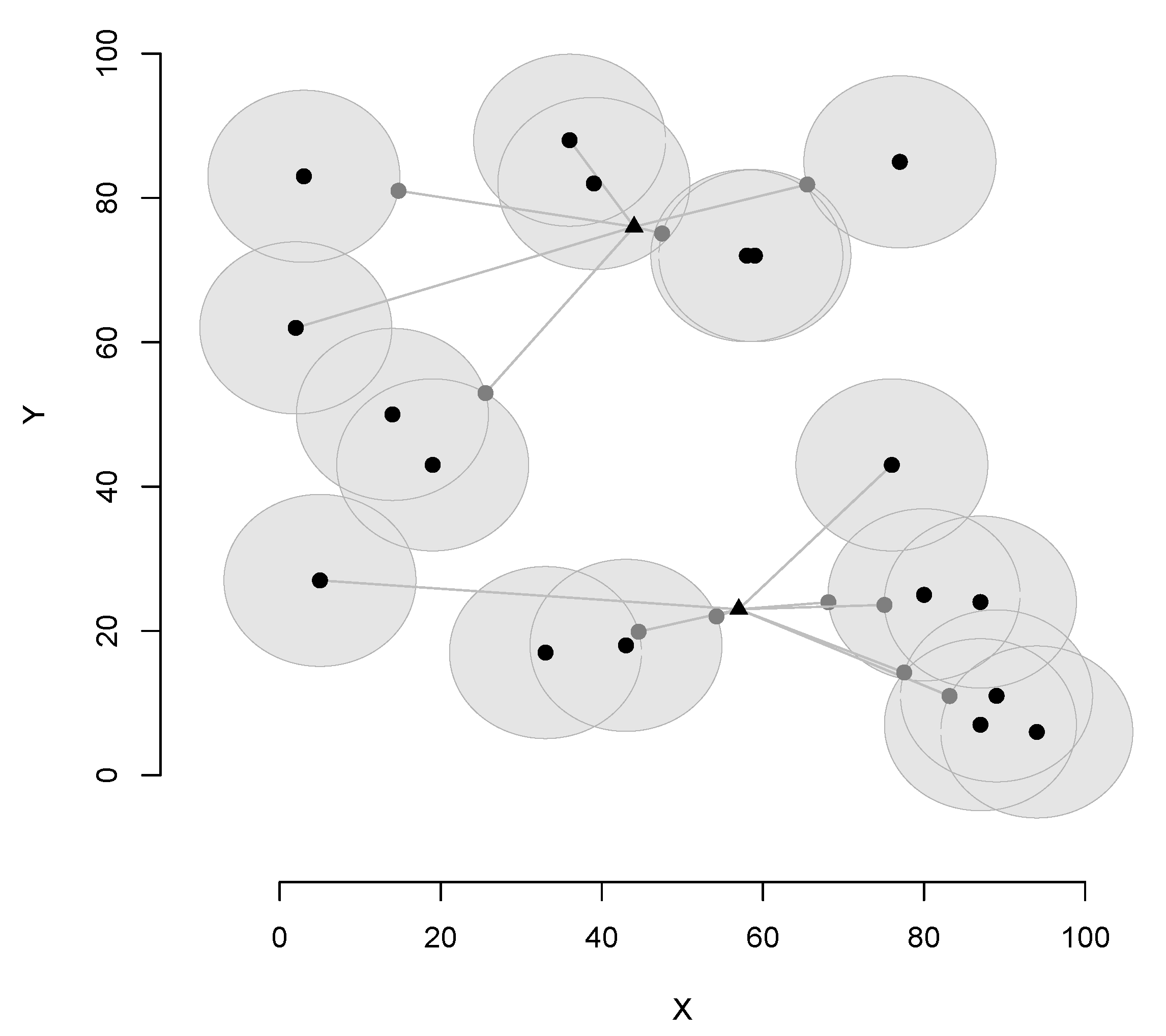
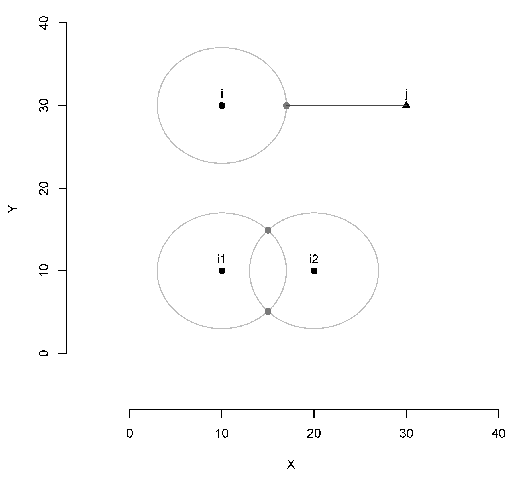
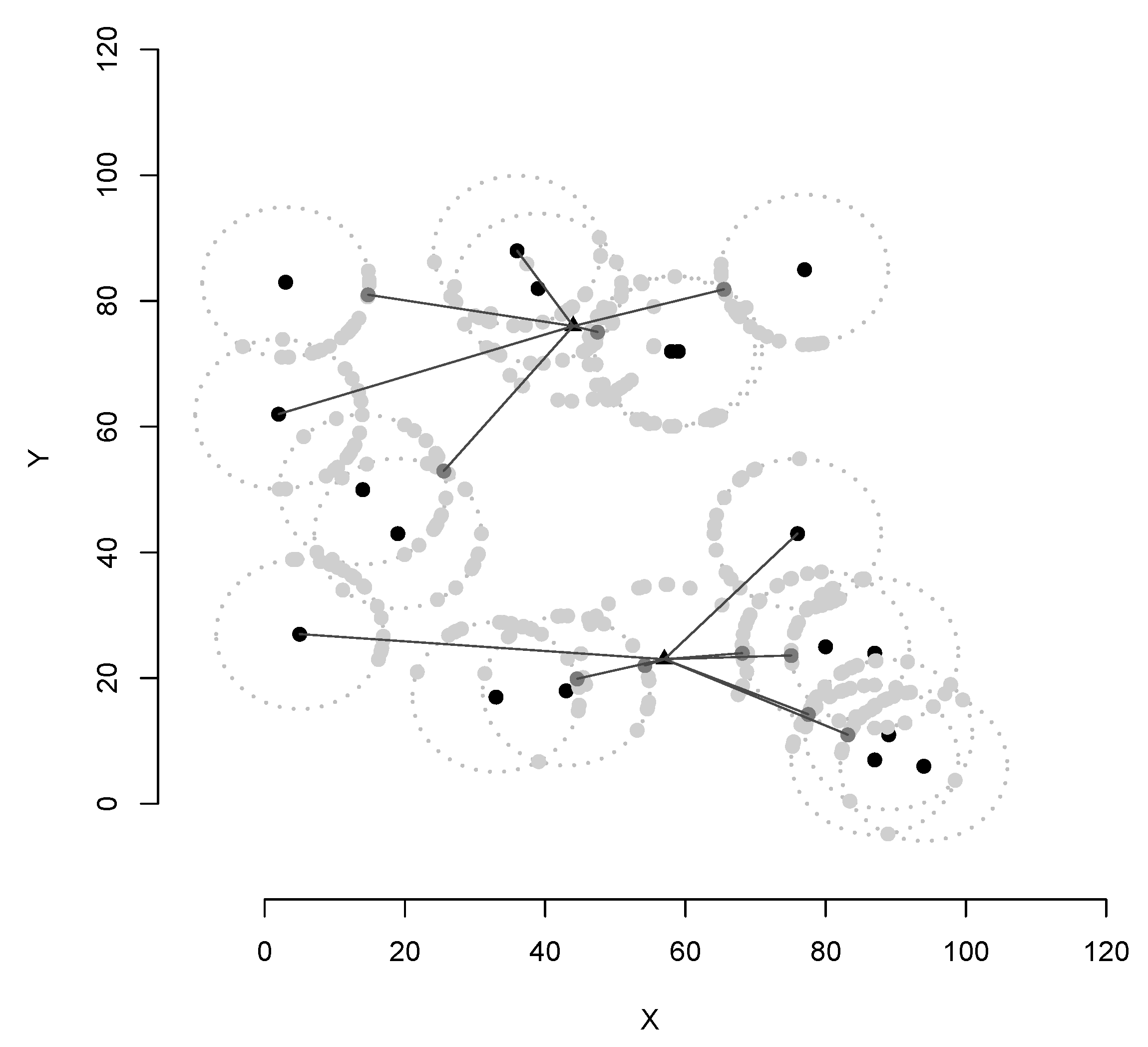
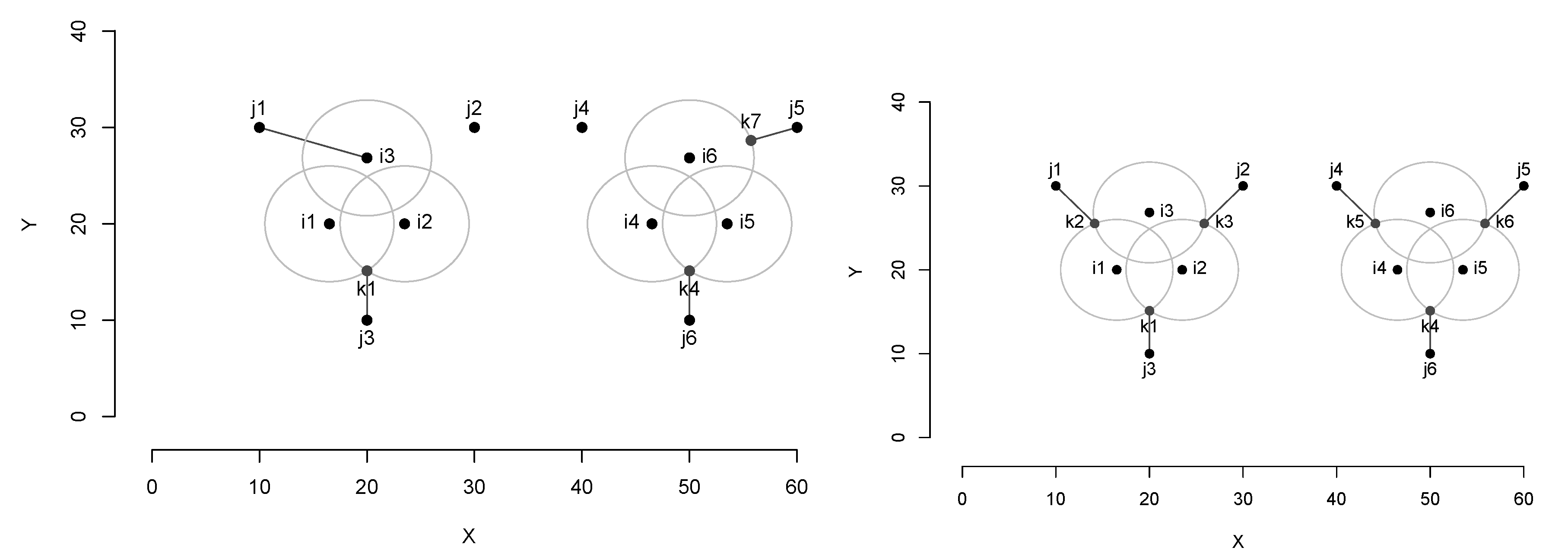
2. Optimal Pickup Locations

In this section it is proved that when minimizing distribution cost, pickup points are never located inside the circles that determine the customers’ areas of movement but at the borders. Even more, pickup points are not located at any point on the circumference but at the intersection of two circumferences or at the intersection of a circumference and a segment connecting one facility and one customer.

The following proposition states that in the optimal solution, the pickup points are always located at the border of customer’s circles. In other words, one pickup point is not an interior point for all the customers.

Let I be the set of customers and J the set of potential facility locations. For each $i\in I,$ let $R_i$ be the distance that customer i is willing to travel to pick up his demand.

Proposition 1.

Let $C_i$ be the set of points in the circumference with centre in customer i and radius $R_i$ and let $S_{ij}$ be the set of points in the segment joining customer i with facility $j.$ Let $(x^{*},y^{*})$ be the coordinates for a pickup point in an optimal solution for the $(p,t)$-CEFLP. Then, one of the following statements hold:

• $(x^{*},y^{*})\in C_i\cap S_{ij}$ for some $i\in I,j\in J.$
• $(x^{*},y^{*})\in C_{i_1}\cap C_{i_2}$ for some $i_1,i_2\in I.$

Proof. 

Let us suppose that $(x^{*},y^{*})$ does not satisfy any of the statements. Let $I^{\prime }$ be the subset of I that moves to $(x^{*},y^{*})$ in the optimal solution. Then, $(x^{*},y^{*})$ belongs to the interior of the area delimited by the intersection of $C_i$ for all $i\in I^{\prime }$ or it is on the border of this area but not at a point of type $C_{i_1}\cap C_{i_2}$ for some $i_1,i_2\in I^{\prime }$ or $C_i\cap S_{ij}$ for some $i\in I^{\prime },j\in J.$ Since the goal is to minimize the distribution cost, $(x^{*},y^{*})$ cannot belong to the interior of the area delimited by the intersection of $C_i$ for all $i\in I^{\prime }:$ the closer $(x^{*},y^{*})$ is to an open facility, the smaller is the distribution cost. Thus, it holds that $(x^{*},y^{*})$

• belongs to $C_{i^{*}}$ for certain $i^{*}\in I$ and $(x^{*},y^{*})$ is on the border of $C_{i^{*}}$.
• is not in $C_{i^{*}}\cap C_i$ for all $i\in I^{\prime }:i\ne i^{*}$.
• and, $(x^{*},y^{*})\notin C_{i^{*}}\cap S_{i^{*}j}$ for all $j\in J.$

Let $j^{*}$ be the facility to which $(x^{*},y^{*})$ is allocated. Then, the solution that replaces $(x^{*},y^{*})$ by $C_{i^{*}}\cap S_{i^{*}{j}^{*}}$ is better than the solution with $(x^{*},y^{*})$ which contradicts that it is optimal.  □

Figure 2 illustrates the two families of candidate pickup locations that Proposition  1 distinguishes—a pickup point is the intersection of a circumsphere and of a segment $C_i\cap S_{ij}$ for some $i\in I$ and $j\in J$ or it is the intersection of two circumferences $C_{i_1}\cap C_{i_2}$ for some $i_1,i_2\in I.$ Pickup points in the figure are the non-labelled gray points.

Proposition  1 entails that the infinite potential set of candidate pickup locations can be reduced to a finite subset. Proposition  1 simplifies the search in the optimization problem by considerably reducing the feasible region so that the problem can be viewed as a discrete location problem and not as a continuous problem.

The cardinality of the finite subset of potential optimal pickup points depends on the relative positions of customers and facilities. From Figure 2, it seems that for each customer-facility pair there is one candidate pickup point and for each pair of customers there are two candidate pickup points. If the distance between two customers $i_1$ and $i_2$ is larger than $R_{i_1}+R_{i_2}$, this pair does not entail a pickup point nor if the distance between a facility j and a customer i is smaller than $R_i.$ The number

$$2\left(\genfrac{}{}{0pt}{}{\left|I\right|}{2}\right)+\left|I\right|\left|J\right|$$

(1)

is un upper bound of the cardinality of the finite subset of potential optimal pickup points.

When the potential facility locations are the customer locations, that is, $I=J$ and $R_i=R$ for all $i,$ the relative position of each pair of elements can be of three types as depicted in Figure 3. Let $d_{i{i}^{\prime }}$ represent the distance between any two points $i,i^{\prime }\in I$ and let $i_1.\dots ,i_6\in I=J$ be six customers/potential facilities. If $d_{i_3{i}_4}>2R,$ then the pair $(i_3,i_4)$ defines two potential pickup points, if $R<d_{i_1{i}_2}<2R$ then the pair $(i_1,i_2)$ defines four potential pickup points and if $d_{i_5{i}_6}<R,$ it defines two. When the radii are different the reasoning is analogous.

Considering $I=J$ in the example in Figure 1, the application of Proposition  1 reduces the feasible region for pickup points from the areas of the circles to the gray points in Figure 4.

3. Notation and Variables

Apart from sets I and J and parameters p and $t,$ in the following sections, we make use of the following sets, parameters and variables. Some of them appear only in Section 4, some only in Section 5 and some in both. For the sake of clarity, we list them all together in this section.

• Sets
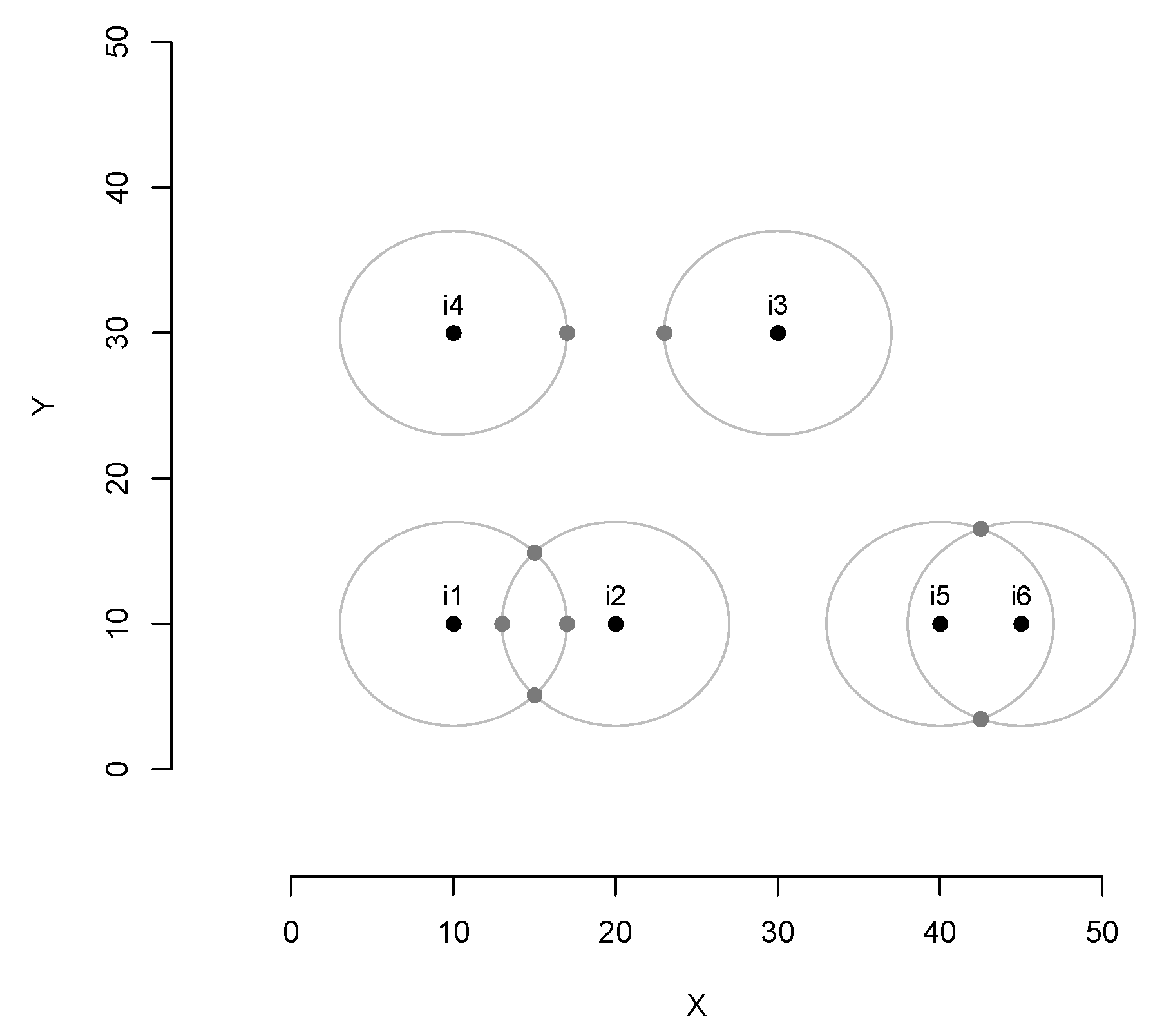
  • K is the set of candidate pickup points induced by Proposition 1, that is, it is the set of circumference intersections and segment-circumference intersections.
  • For all $i\in I,$$K_i$ is the subset of K that customer i could benefit from, $K_i$ is the set of elements k of K such that $d_{ik}\le R_i.$$K_i$ and $K_j$ might overlap and K is the union of $K_i$ for all $i\in I.$
  • For all $i\in I,$${\overline{K}}_i$ is the subset of $K_i$ in the border, that is, the set of elements k of K such that $d_{ik}=R_i.$
  • For all $k\in K,$$I_k$ is the set of customers that are willing to move to $k,$ that is, $I_k=\{i\in I:d_{ik}\le R_i\}.$
• Parameters
  • For all $i\in I,$$h_i$ is the demand of customer $i.$
  • For all $i\in I,$$R_i$ is the distance that customer i is willing to travel for picking up his demand. It is named R when $R_{i_1}=R_{i_2}$ for all $i_1.i_2\in I.$
  • For each $i\in I,j\in J,$$d_{ij}$ is the distance between i and $j.$
  • For each $k\in K,j\in J,$$d_{kj}$ is the distance between k and $j.$
• Variables
  • For all $j\in J,$$y_j\in \{0,1\}$ is 1 if facility j is open.
  • For all $k\in K,$${\nu }_k\in \{0,1\}$ is 1 if the pickup point k is installed.
  • For all $i\in I,$$j\in J,$$x_{ij}\in \{0,1\}$ is 1 if customer i is allocated to facility j,
  • For all $i\in I,$$k\in K,$$z_{ik}\in \{0,1\}$, is 1 if customer i moves to the pickup location $k,$
  • For all $k\in K,$$j\in J,$$s_{kj}\ge 0$ is the demand supported by facility j through the pickup point $k.$
  • For all $i\in I,$$k\in K,$$j\in J,$$w_{ikj}\in \{0,1\}$ is 1 if customer i moves to the pickup location k and facility j serves the pickup point $k,$$w_{iij}=1$ represents that customer i is directly served from facility j and thus, does not move to any pickup point.

Both two-index variables and three-index variables are frequently used when modelling location problems, sometimes even four-index variables, see for instance [13,14,15,16] among others.

The Binary Integer Variables

Since the $(p,t)$-CEFLP lacks capacity constraints, once the decision of where to locate the p facilities and the t pickup points is taken, the customers’ allocation is straightforward—customers pickup their goods at some pickup point as long as it is within their radius or customers pickup their goods at the nearest facility. Thus, provided that $y_j\in \{0,1\}$ for all $j\in J$ and ${\nu }_k\in \{0,1\}$ for all $k\in K,$ variables $x_{ij},$$z_{ik}$ and $w_{ikj}$ would take integer values, even if their domains became $[0,1].$ Conversely, the location of the pickup points is nontrivial with regard to facility location. In this section, we show that the problem of locating the pickup points when the number of open facilities is known is still difficult, in the sense that if the constraint ${\nu }_k\in \{0,1\}$ is replaced by the constraint ${\nu }_k\in [0,1],$ the optimal solution changes and it might happen that a solution with fractional pickup locations would be cheaper than any binary solution.

Let us consider the situation depicted in Figure 5. There are six customers $I=\{i_1,i_2,i_3,i_4,i_5,i_6\}$ at coordinates $i_1=(16.51,20),i_2=(23.5,20),i_3=(20,26.84),i_4=(46.51,20),i_5=(53.5,20),i_6=(50,26.84),$ and six potential facilities $J=\{j_1,j_2,j_3,j_4,j_5,j_6\},$ at coordinates $j_1=(10,30),j_2=(30,30),j_3=(20,10),j_4=(40,300),j_5=(60,30),j_6=(50,10)$ and the radius is $R_i=6$ for all $i\in I.$ The best solution for $p=6$ and $t=3$ consists of opening all the plants and the pickup locations $k1,$$k4$ and $k7$, entailing a cost of 35.46: customers $i1$ and $i2$ move to pickup location $k1$ which is allocated to facility $j3,$ customer $i3$ does not move to any pickup location but moves to facility $j1,$ customers $i4,$$i5$ move to pickup location $k4$ which is allocated to facility $j6$ and customer $i6$ moves to the pickup location $k7$, which is allocated to facility $j5.$ If fractional pickup points could be opened, the solution with ${\nu }_{k_1}={\nu }_{k_2}={\nu }_{k_3}={\nu }_{k_4}={\nu }_{k_5}={\nu }_{k_6}=0.5$ would be better with a cost of 34.68. The circumsphere and segment intersections give a set of 169 potential pickup points. However, and for the sake of clarity, we have only depicted the seven pickup points in the two considered solutions. Note that these six customers and facilities could be part of a larger problem with more customers and facilities and it would justify that in the integer solution facilities, $j2$ and $j4$ are open but do not serve customers.

4. Mixed-Integer Linear Two-Index Formulation

The $(p,t)$-CEFLP can be modelled as follows.

$$\begin{array}{cc}\hfill \left(P_1\right)min& {\displaystyle \sum _{i\in I}\sum _{j\in J}{h}_i{d}_{ij}{x}_{ij}+\sum _{k\in K}\sum _{j\in J}{d}_{kj}{s}_{kj}}\end{array}$$

(2)

$$\begin{array}{ccc}\hfill st& {\displaystyle \sum _{j\in J}{y}_j=p}& \hfill \end{array}$$

(3)

$$\begin{array}{ccc}& {\sum }_{k\in K}{\nu }_k=t& \hfill \end{array}$$

(4)

$$\begin{array}{ccc}& {\displaystyle \sum _{j\in J}{x}_{ij}+\sum _{k\in K_i}{z}_{ik}=1}& \forall i\in I\hfill \end{array}$$

(5)

$$\begin{array}{ccc}& {\displaystyle \sum _{j\in J}{s}_{kj}=\sum _{i\in I_k}{h}_i{z}_{ik}}& \forall k\in K\hfill \end{array}$$

(6)

$$\begin{array}{ccc}& {\displaystyle \sum _{k\in K}{s}_{kj}\le M{y}_j}& \forall j\in J\hfill \end{array}$$

(7)

$$\begin{array}{ccc}& {\displaystyle z_{ik}\le {\nu }_k}& \forall i\in I,k\in K_i\hfill \end{array}$$

(8)

$$\begin{array}{ccc}& {\displaystyle x_{ij}\le y_j}& \forall i\in I,j\in J\hfill \end{array}$$

(9)

$$\begin{array}{ccc}& x_{ij}\in \{0,1\}& \forall i\in I,j\in J\hfill \end{array}$$

(10)

$$\begin{array}{ccc}& z_{ik}\in \{0,1\}& \forall i\in I,k\in K_i\hfill \end{array}$$

(11)

$$\begin{array}{ccc}& y_j\in \{0,1\}& \forall j\in J\hfill \end{array}$$

(12)

$$\begin{array}{ccc}& {\nu }_k\in \{0,1\}& \forall k\in K\hfill \end{array}$$

(13)

$$\begin{array}{ccc}& s_{kj}\ge 0& \forall k\in K,j\in J.\hfill \end{array}$$

(14)

The objective function measures the total cost; the first term is the cost of satisfying the demand of those customers that do not make use of pickup points but are directly served from facilities and the second term is the cost of sending goods from open facilities to open pickup points. Constraint (3) states that the number of open facilities is p and constraint (4) that the number of open pickup points is $t.$ Constraints (5) guarantee that all the customers move to a pickup point or are directly served by an open facility. Constraint (6) computes the amount of product that an open pickup point k distributes. Constraints (7) and (8) entail that pickup points must be served from open facilities and constraints (9) that customers that do not make use of pickup points are served from open facilities. M is any upper bound for the values of ${\sum }_{k\in K}{s}_{kj},$ that is, any upper bound for the demand supported by one facility: in practice, it is the addition of all the customer’s demand, $M={\sum }_{i\in I}{h}_i.$ Constraints (10)–(14) are the domain constraints.

Polyhedral Enhancement

Some valid inequalities follow from the analysis of the problem that make the model strong.

Proposition 2.

For all $i\in I,$ the following inequalities are valid inequalities for $P_1.$

$$\begin{array}{cc}& {\displaystyle \sum _{j\in J}{x}_{ij}+\sum _{k\in K_i\backslash {\overline{K}}_i}{z}_{ik}+\sum _{k\in {\overline{K}}_i}{\nu }_k\le 1.}\end{array}$$

(15)

Proof. 

If customer i is allocated to a facility, then does not move to any of the pickup points at $K_i\backslash {\overline{K}}_i$ and if does move to a pickup point at $K_i\backslash {\overline{K}}_i,$ then the pickup points at ${\overline{K}}_i$ are closed.  □

Proposition 3.

For all $i\in I$ and $j\in J,$ let $k(i,j)$ be the pickup point in $C_i\cap S_{ij}.$ Then, it holds that the inequalities

$$\begin{array}{ccc}& {\nu }_{k(i,j)}\le y_j& \forall j\in J\forall i\in I\hfill \end{array}$$

(16)

are valid inequalities for $P_1.$

Proof. 

If facility j is closed, none of the pickup points allocated to it can be open.  □

Remark 1.

If $I=J,$ then it holds that $y_i=x_{ii}$ for all $i.$

Corollary 1.

For all $i_1,i_2\in I$ such that $d_{i_1,i_2}<R_{i_1}+R_{i_2},$ let $k_1(i_1,i_2)$ and $k_2(i_1,i_2)$ be the two points in $C_{i_1}\cap C_{i_2}.$ If $I=J,$ then it holds that the inequalities

$$\begin{array}{cc}\hfill \sum _{j\in J:j\ne i_1}{x}_{i_{1}j}+{\nu }_{k_1(i_1,i_2)}+{\nu }_{k_2(i_1,i_2)}+{\nu }_{k(i_1,i_2)}+{\nu }_{k(i_2,i_1)}\le 1& \forall i_1,i_2\in I,d_{i_1,i_2}<R_{i_1}+R_{i_2}\end{array}$$

(17)

$$\begin{array}{cc}\hfill \sum _{j\in J:j\ne i_2}{x}_{i_{2}j}+{\nu }_{k_1(i_1,i_2)}+{\nu }_{k_2(i_1,i_2)}+{\nu }_{k(i_1,i_2)}+{\nu }_{k(i_2,i_1)}\le 1& \forall i_1,i_2\in I,d_{i_1,i_2}<R_{i_1}+R_{i_2}\end{array}$$

(18)

are valid inequalities for $P_1.$

Proof. 

If ${\sum }_{j\in J:j\ne i_1}{x}_{i_{1}j}=1,$ then $x_{i_1{i}_1}=y_{i_1}=0$ and from inequality (16), it holds that ${\nu }_{k(i_2,i_1)}=0.$ The rest follows from inequality (15). It is analogous when ${\sum }_{j\in J:j\ne i_2}{x}_{i_{2}j}=1.$  □

Remark 2.

Allocation variables $z_{ik}$ commonly appear in discrete location models. However, only some of the valid inequalities in the literature for this family can be used for $P_1.$ In fact, we point out that the inequality

$$\begin{array}{c}\hfill \sum _{i\in I_k}{z}_{ik}\le min\left\{\right(\left|I\right|-t+1),|I_k\left|\right\}{\nu }_k\forall k\in K,\end{array}$$

(19)

which is based on the one proposed by [17], is valid for $P_1.$ The rest of inequalities in literature for variables $z_{ik}$ which are surveyed in [18] do not apply because $I⊈K.$

5. Mixed-Integer Linear Three-Index Formulation

The $(p,t)$-CEFLP can be alternatively modeled as follows.

$$\begin{array}{ccc}\hfill \left(P_2\right)min& {\displaystyle \sum _{i\in I}\sum _{k\in K_i\cup \left\{i\right\}}\sum _{j\in J}{h}_i{d}_{kj}{w}_{ikj}}& \hfill \\ \hfill \mathrm{s}.\mathrm{t}& \left(3\right),\left(4\right)& \hfill \end{array}$$

(20)

$$\begin{array}{ccc}& {\displaystyle \sum _{j\in J}\sum _{k\in K_i\cup \left\{i\right\}}{w}_{ikj}=1}& \forall i\in I\hfill \end{array}$$

(21)

$$\begin{array}{ccc}& {\displaystyle \sum _{j\in J}{w}_{ikj}\le {\nu }_k}& i\in I,k\in K_i\hfill \end{array}$$

(22)

$$\begin{array}{ccc}& {\displaystyle \sum _{k\in K_i\cup \left\{i\right\}}{w}_{ikj}\le y_j}& \forall i\in I,j\in J\hfill \end{array}$$

(23)

$$\begin{array}{ccc}& w_{ikj}\in \{0,1\}& \forall i\in I,k\in K_i\cup \left\{i\right\},j\in J\hfill \end{array}$$

(24)

$$\begin{array}{ccc}& y_j\in \{0,1\}& \forall j\in J\hfill \end{array}$$

(25)

$$\begin{array}{ccc}& {\nu }_k\in \{0,1\}& \forall k\in K.\hfill \end{array}$$

(26)

The objective function is again the total cost, the cost of satisfying the demand of those customers that do not make use of pickup points plus the cost of sending goods from open facilities to open pickup points. Constraints (21) guarantee that all the customers are served, constraints (22) that only open pickup points can deliver goods and constraints (23) that only open facilities can serve pickup points and customers. Finally, constraints (24)–(26) are the domain constraints.

Remark 3.

Valid inequalities (16) apply and strengthen $P_2.$

Inequalities (15) and (19) and inequalities in Corollary  1 can be easily adapted as stated in the following remark.

Remark 4.

Since $x_{ij}$ in $P_1$ is $w_{iij}$ in $P_2$ and $z_{ik}={\sum }_{j\in J}{w}_{ijk},$ the following inequalities are valid for $P_2.$

$$\begin{array}{c}\hfill {\displaystyle \sum _{j\in J}{w}_{iij}+\sum _{j\in J}\sum _{k\in K_i\backslash {\overline{K}}_i}{w}_{ikj}+\sum _{k\in {\overline{K}}_i}{\nu }_k\le 1}\\ \hfill \sum _{i\in I}\sum _{j\in J}{w}_{ijk}\le min\left\{\right(\left|I\right|-t+1),|I_k\left|\right\}{\nu }_k\forall k\in K\end{array}$$

If $I=J,$ then it holds that the inequalities

$$\begin{array}{cc}\hfill \sum _{j\in J:j\ne i_1}{w}_{i_1{i}_{1}j}+{\nu }_{k_1(i_1,i_2)}+{\nu }_{k_2(i_1,i_2)}+{\nu }_{k(i_1,i_2)}+{\nu }_{k(i_2,i_1)}\le 1& \forall i_1,i_2\in I,d_{i_1,i_2}<R_{i_1}+R_{i_2}\\ \hfill \sum _{j\in J:j\ne i_2}{w}_{i_2{i}_{2}j}+{\nu }_{k_1(i_1,i_2)}+{\nu }_{k_2(i_1,i_2)}+{\nu }_{k(i_1,i_2)}+{\nu }_{k(i_2,i_1)}\le 1& \forall i_1,i_2\in I,d_{i_1,i_2}<R_{i_1}+R_{i_2}\end{array}$$

are valid inequalities for $P_2.$

It is not difficult to prove that the LP gap of $P_2$ is smaller than the LP gap of $P_1.$ that is, that the linear relaxation of $P_2$ gives larger objective values than the linear relaxation of $P_1.$

Proposition 4.

Let $v^{*}\left(P_1^{LR}\right)$ be the optimal value of the linear relaxation of $P_1$ and $v^{*}\left(P_2^{LR}\right)$ be the optimal value of the linear relaxation of $P_2.$ It holds $v^{*}\left(P_1^{LR}\right)\le v^{*}\left(P_2^{LR}\right).$

Proof. 

It is clear that $x_{ij}=w_{iij}$ and that $z_{ik}={\sum }_{j\in J}{w}_{ijk}.$ Accordingly, replacing $z_{ik}$ in (6), that is,

$$\sum _{j\in J}{s}_{kj}=\sum _{j\in J}\sum _{i\in I_k}{h}_i{w}_{jk},$$

it follows that $s_{kj}={\sum }_{i\in I_k}{h}_i{w}_{jk}.$ Thus, the three families of variables in $P_1,$$x_{ij},z_{ik}$ and $s_{kj}$ can be written in terms of the variables in $P_2,$ that is, $w_{ijk}.$ By using these identities, constraints (5) become constraints (21), constraints (6) are the $s_{kj}$ definitions, constraints (8) become constraints (22), constraints (9) is a subset of constraints in (23) and (7) become

$$\sum _{k\in K}\sum _{i\in I_k}{h}_i{w}_{jk}\le M{y}_j$$

which is a linear combination of constraints (23) with weights $h_i$ and $M={\sum }_{i\in I}{h}_i.$  □

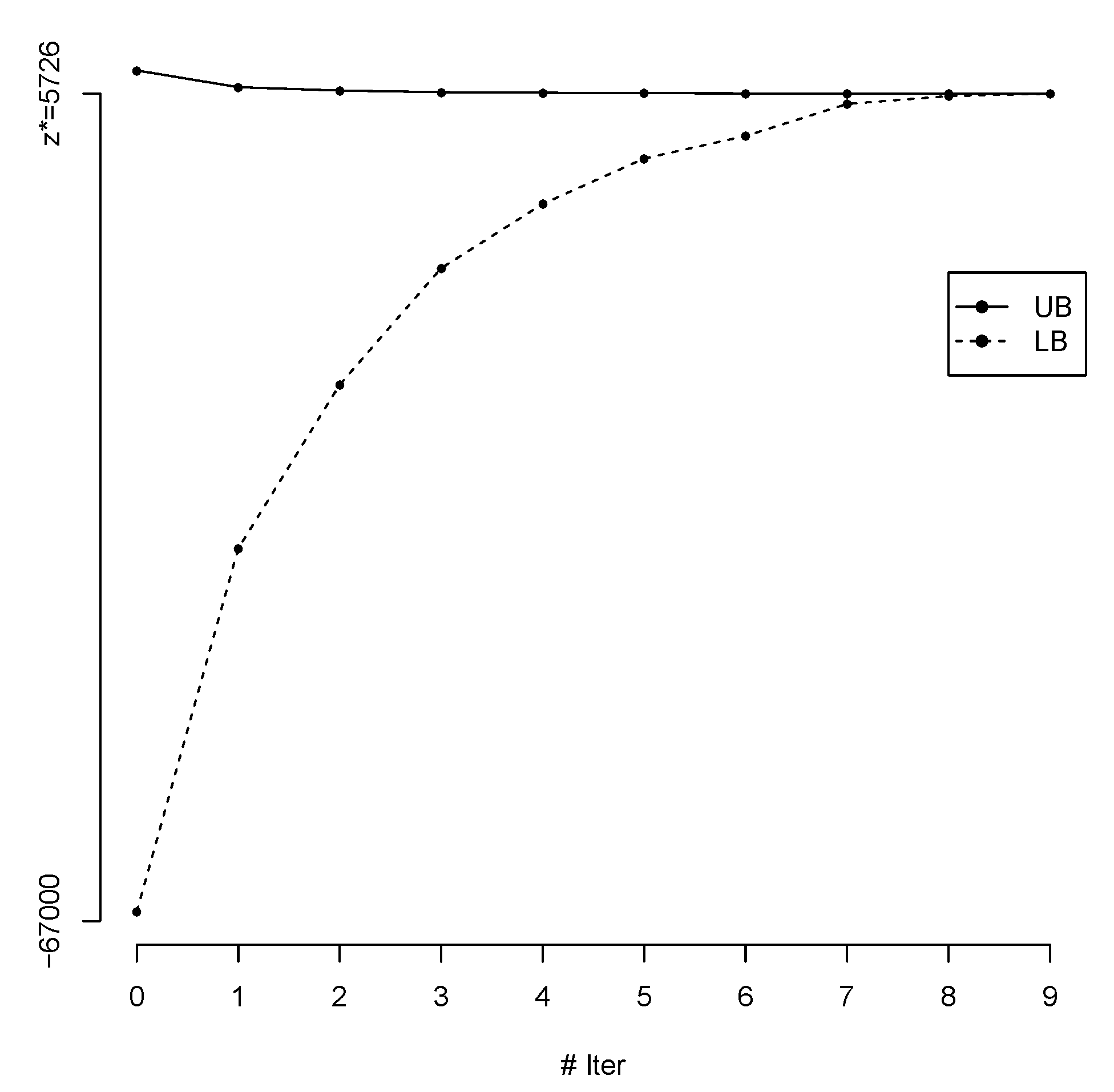
Branch and Price Algorithm

The $P_2$ formulation has a very small integrality gap but it has a huge number of variables. Both facts together suggest that a column generation approach is a promising resolution method. Column generation is a popular approach when handling models with a lot variables that have good performance in terms of integrality gap, see [19] for an application to the discrete ordered median problem and [20,21,22,23] for solving different combinatorial problems.

Let $(\delta ,\theta ,{\alpha }_i,{\beta }_{ik},{\gamma }_{ij})$ be the dual variables of constraints (3), (4), (21), (22) and (23) respectively. The dual problem for the linear relaxation of $P_2$ is the following Linear Relaxation Master Problem (LRMP).

$$\begin{array}{ccc}\hfill \left(\mathrm{LRMP}\right)max& {\displaystyle p\delta +t\theta +\sum _{i\in I}{\alpha }_i}& \hfill \\ \hfill s.t.& {\displaystyle {\alpha }_i+{\beta }_{ik}+{\gamma }_{ij}\le h_i{d}_{kj}}& \forall j\in J,i\in I,k\in K_i\hfill \\ & {\displaystyle \delta -\sum _{i\in I}{\gamma }_{ij}\le 0}& \forall j\in J\hfill \\ & {\displaystyle \theta -\sum _{i\in I_k}{\beta }_{ik}\le 0}& \forall k\in K\hfill \\ & {\beta }_{ik}\le 0& \forall i\in I,k\in K\hfill \\ & {\gamma }_{ij}\le 0& \forall i\in I,j\in J\hfill \\ & {\alpha }_i\mathrm{free}& \forall i\in I\hfill \\ & \delta ,\theta .\mathrm{free}\end{array}$$

In order to apply the column generation approach, let us assume that we are given a subset of intersection points $\widehat{K}\subset K$ that defines a restricted linear relaxation of the Master Problem, from now on ReLRMP. Let $({\delta }^{*},{\theta }^{*},{\alpha }^{*},{\beta }^{*},{\gamma }^{*})$ be the optimal solution of ReLPMP. Then, the reduced cost ${\tilde{c}}_k$ of the column ${\nu }_k$ for all $k\in K\backslash \widehat{K}$ is

$${\tilde{c}}_k=\sum _{i\in I_k}{\beta }_{ik}-{\theta }^{*}$$

where

$${\beta }_{ik}\le h_i{d}_{kj}-{\alpha }_i^{*}-{\gamma }_{ij}^{*},\forall j\in J,i\in I_k.$$

The pricing subproblem, the problem of obtaining the maximum value for ${\tilde{c}}_k,$ can be directly obtained without optimizing.

Proposition 5.

Let $({\delta }^{*},{\theta }^{*},{\alpha }^{*},{\beta }^{*},{\gamma }^{*})$ be the optimal solution of ReLPMP for $\widehat{K}\subset K$. Then, the maximum reduced cost ${\overline{c}}_k$ of the column ${\nu }_k$ is

$${\overline{c}}_k=\sum _{i\in I_k}\underset{j\in J}{min}\{h_i{d}_{kj}-{\alpha }_i^{*}-{\gamma }_{ij}^{*}\}-{\theta }^{*},\forall k\in K\backslash \widehat{K}.$$

Proof. 

It follows from maximizing ${\sum }_{i\in I_k}{\beta }_{ik}-{\theta }^{*}$ subject to ${\beta }_{ik}\le h_i{d}_{kj}-{\alpha }_i^{*}-{\gamma }_{ij}^{*}$ for all $j\in J,i\in I_k.$  □

${\overline{c}}_k$ is an estimation of the improvement in the objective function if the pickup point k is introduced in ReLRMP. If ${\overline{c}}_k\le 0$ for all $k\in K\backslash \widehat{K}$, the current solution of ReLRMP is also optimal for the LRMP and the column generation approach is finished. Otherwise, each positive value proposes the addition of a new column (variable) to the current reduced master problem to proceed further. In each iteration, the optimal value of ReLRMP, $z_{ReLRMP},$ not only gives an upper bound of the optimal value of LRMP, $z_{LRMP}$, but also a lower bound of it. $z_{LRMP}$ cannot be reduced more than the smaller reduced cost ${\overline{c}}_k$ for each customer i if $k\in K_i,$ hence

$$z_{ReLRMP}+\sum _{i\in I}\underset{k\in K_i}{min}{\overline{c}}_k\le z_{LRMP}\le z_{ReLRMP}.$$

Algorithm 1 clearly describes the branch and price procedure that we propose. $K_0$ is a subset of K, such that $K_0\cap K_i\ne \varnothing$ for all $i\in I,$ ideally $K_0$ has exactly one element from each $K_i.$

Algorithm 1: Branch and price algorithm

6. Computational Results

In this section, the performance of the two linear formulations as well as the performance of the polyhedral enhancement and of the branch and price algorithm is illustrated. The experiment has been coded in C++, using IBM ILOG CPLEX Optimization Studio. The characteristics of the computer are an 8 GB RAM and an Intel Core i5 2 GHz processor. The default options of CPLEX v12.8 have been used for solving the models $P_1$ and $P_2$ as well for solving the submodels in the branch and price algorithm.

For the computational experiments, we have used the pmedcap1.txt file, which contains the problems solved in [24], originally generated for the p-median problem. It always holds that $I=J,$ that is, customers are the potential facility locations. From the instances in pmedcap1.txt, we have defined 60 different instances for our problem with constant radius. The number of facilities and pickup points has been decided by the graphic distribution of the points.

Table 1. Data instances and $P_1$ and $P_2$ dimensions.

Instance	Data Instances					${\mathit{P}}_1$			${\mathit{P}}_2$
	n	p	t	R	$\#\mathit{k}$	m	$\mathit{n}01$	$\mathbf{nc}$	m	$\mathit{n}01$
i1	10	2	3	2.69	90	312	300	1000	202	1100
i2	20	2	10	2.98	382	1253	1231	8040	831	8982
i3	30	3	10	2.98	874	2821	2789	27120	1887	30454
i4	35	3	10	2.98	1196	3841	3804	43085	2575	48411
i5	40	4	10	2.98	1568	5047	5005	64320	3399	73488
i6	50	4	10	2.98	2462	7885	7833	125600	5323	143562
i7	55	4	10	3.25	2984	9550	9493	167145	6456	191634
i8	60	4	10	3.25	3560	11493	11431	217200	7813	256280
i9	65	4	10	3.25	4186	13552	13485	276315	9236	329836
i10	70	4	10	3.25	4858	15765	15693	344960	10767	415478
i11	75	4	10	3.25	5588	18152	18075	424725	12414	514688
i12	80	4	10	3.25	6362	20645	20563	515360	14123	624122
i13	85	4	10	3.25	7190	23366	23279	618375	16006	753490
i14	90	4	10	3.25	8068	26555	26463	734220	18307	926608
i15	100	4	10	3.25	9974	33197	33095	1007400	23023	1312174
i16	10	2	3	5.39	92	328	316	1020	216	1242
i17	20	2	10	5.96	394	1408	1386	8280	974	11854
i18	30	3	10	5.96	894	3139	3107	27720	2185	39414
i19	35	3	10	5.96	1222	4304	4267	43995	3012	63732
i20	40	4	10	5.96	1608	5806	5764	65920	4118	102288
i21	50	4	10	5.96	2522	9165	9113	128600	6543	204622
i22	55	4	10	6.51	3092	11693	11636	173085	8491	303667
i23	60	4	10	6.51	3686	14299	14237	224760	10493	417206
i24	65	4	10	6.51	4332	17253	17186	285805	12791	561057
i25	70	4	10	6.51	5030	20297	20225	357000	15127	720850
i26	75	4	10	6.51	5774	23633	23556	438675	17709	911999
i27	80	4	10	6.51	6570	27116	27034	532000	20386	1125370
i28	85	4	10	6.51	7424	30973	30886	638265	23379	1380429
i29	90	4	10	6.51	8322	35594	35502	757080	27092	1717512
i30	100	4	10	6.51	10294	45371	45269	1039400	34877	2497894
i31	10	2	3	10.77	94	352	340	1040	238	1464
i32	20	2	10	11.92	420	1786	1764	8800	1326	18920
i33	30	3	10	11.92	962	4299	4267	29760	3277	72242
i34	35	3	10	11.92	1306	5976	5939	46935	4600	119396
i35	40	4	10	11.92	1724	8513	8471	70560	6709	206044
i36	50	4	10	11.92	2704	14364	14312	137700	11560	455654
i37	55	4	10	13.01	3324	19843	19786	185845	16409	739389
i38	60	4	10	13.01	3978	25449	25387	242280	21351	1068978
i39	65	4	10	13.01	4664	31095	31028	307385	26301	1439539
i40	70	4	10	13.01	5420	37459	37387	384300	31899	1895280
i41	75	4	10	13.01	6256	45666	45589	474825	39260	2528806
i42	80	4	10	13.01	7094	52542	52460	573920	45288	3118054
i43	85	4	10	13.01	7992	60791	60704	686545	52629	3867247
i44	90	4	10	13.01	8964	70554	70462	814860	61410	4806774
i45	100	4	10	13.01	11086	93774	93672	1118600	82488	7259786
i46	10	2	3	16.16	106	433	421	1160	307	2166
i47	20	2	10	17.88	442	2203	2181	9240	1721	26842
i48	30	3	10	17.88	1032	6064	6032	31860	4972	123162
i49	35	3	10	17.88	1396	8617	8580	50085	7151	208771
i50	40	4	10	17.88	1844	12645	12603	75360	10721	366644
i51	50	4	10	17.88	2862	21290	21238	145600	18328	794212
i52	55	4	10	19.52	3636	34148	34091	203005	30402	1509316
i53	60	4	10	19.52	4352	44494	44432	264720	40022	2189612
i54	65	4	10	19.52	5116	55680	55613	336765	50434	3008636
i55	70	4	10	19.52	5972	69046	68974	422940	62934	4068282
i56	75	4	10	19.52	6866	84296	84219	520575	77280	5380916
i57	80	4	10	19.52	7822	98965	98883	632160	90983	6774382
i58	85	4	10	19.52	8794	114545	114458	754715	105581	8368969
i59	90	4	10	19.52	9896	135054	134962	898740	124978	10528826
i60	100	4	10	19.52	12222	181436	181334	1232200	169014	15913522

describes the 60 different instances we have used in this section. We call n the number of potential facilities and/or customers, that is, $n=\left|I\right|=\left|J\right|.$ Instances i1-i6, i16-i21, i31-i36 and i46-i51 follow from the corresponding first n nodes of the first instance in pmedcap1.tx1 with 50 nodes, instances i7-i15, i22-i30, i37-i45 and i52-i60 follow from the corresponding first n nodes of the first instance in pmedcap1.tx1 with 100 nodes. Instances i16-i30 have the same data as instances i1-i15 but with a different value for $R.$ Instances i31-i45 are also i1-i15 for another radius, and so on. For each instance, we have fixed values for $p,$t and R as shown in Table 1. The radius is constant at each instance. The radius for i1-i15 is the 2.5% of the maximum euclidean distance between nodes in the instance; the radius for i16-i30 is 5% this maximum and the radius for i31-i45 and i46-i60 is 10% and 15% respectively. Column $\#k$ gives the size of the set $K.$ Note that when R is small, $\left|K\right|$ is farther form the upper bound (1) than when R is medium: i1, i16, i31 and i46 differ in R and $\left|K\right|$ grows as R does: the bound $2\left(\genfrac{}{}{0pt}{}{\left|I\right|}{2}\right)+\left|I\right|\left|J\right|$ is $2\left(\genfrac{}{}{0pt}{}{10}{2}\right)+10\ast 10=190$ while $\left|K\right|$ goes from 90 to 106. Similarly, for all the 4-uples of instances with the same data but different radii, iq, i$q+15$, i$q+30$, i$q+45$ for all $q\in \{1.\dots ,15\}.$ For $q=15,$$\left|K\right|$ varies in $\{9974,10294,11086,12222\}.$

Table 1 also shows the $P_1$ and $P_2$ dimensions for the 60 chosen instances. For each instance, it shows the number of constraints of the model (m), the number of 0-1 variables ($n01$) and the number of continuous variables ($nc$). Table 1 corroborates that $P_1$ has more rows but significantly less variables than $P_2$. The number of variables in $P_1$ when solving i60 is smaller than the number of variables in $P_1$ when solving i15. In the following, we shall see that within a two-hour time-limit, we successfully solved 16 of 60 instances with $P_1$ and 57 with $P_2.$

In the sequel we split the computational results into two subsections. In the first one, the two optimization models are compared, in the second one, the best of the two optimization models is compared with the branch and price algorithm.

6.1. Optimization Models Results

Table 2. $P_1,$ enhanced $P_1$ and $P_2$.

Instance	${\mathit{P}}_1$			${\mathit{P}}_1+$(15)		${\mathit{P}}_1+$(16)		${\mathit{P}}_1+$(17)+(18)		${\mathit{P}}_1+$(19)		${\mathit{P}}_1+$(15)+…+(18)		${\mathit{P}}_2$
	$\mathit{Obj}$	$\mathit{Time}$$(\mathit{s}.)$	$\mathit{GAP}$ %	$\mathit{Time}$$(\mathit{s}.)$	$\mathit{GAP}$ %	$\mathit{Time}$	$\mathit{GAP}$ %	$\mathit{Time}$$(\mathit{s}.)$	$\mathit{GAP}$ %	$\mathit{Time}$$(\mathit{s}.)$	$\mathit{GAP}$ %	$\mathit{Time}$$(\mathit{s}.)$	$\mathit{GAP}$ %	$\mathit{Time}$$(\mathit{s}.)$	$\mathit{GAP}$ %
i1	1600.86	1	62.90	0	62.90	1	61.65	0	62.00	1	62.90	0	61.65	0.00	0.00
i2	4771.03	88	82.26	28	82.26	12	81.79	46	82.15	72	82.26	10	81.79	0.00	0.00
i3	5364.57	485	65.32	550	65.32	223	64.61	981	64.98	3926	65.32	323	64.61	1.00	0.00
i4	6534.84	1032	60.08	1153	60.08	1418	58.60	3699	59.48	4633	60.08	1279	58.60	1.00	0.00
i5	5359.16	3463	52.99	7069	52.99	5747	51.97	7200	52.57	7200	52.99	4916	51.97	2.00	0.00
i16	1493.16	0	58.06	1	58.06	0	56.68	1	57.29	0	58.06	0	56.68	0.00	0.00
i17	4309.60	70	85.63	75	85.63	22	85.28	88	85.62	44	85.63	21	85.28	0.00	0.00
i18	4837.41	764	67.28	1135	67.28	979	66.64	1344	67.10	2056	67.28	831	66.64	1.00	0.00
i19	6011.42	7200	66.29	1715	66.29	3177	65.25	4335	66.03	5331	66.29	1793	65.25	1.00	0.00
i20	4681.10	7200	58.20	7200	58.19	7200	56.80	7200	57.91	7200	58.19	7034	56.80	2.00	0.00
i31	1258.92	0	41.82	1	41.82	0	39.30	1	41.41	1	41.82	0	39.30	0.00	0.00
i32	3369.58	99	84.53	127	84.39	48	82.54	92	84.53	89	84.53	28	81.98	1.00	0.00
i33	1891.92	1965	91.69	5566	91.69	1902	89.98	1446	91.69	2162	91.69	3667	89.97	2.00	0.29
i34	2666.33	4788	92.61	7200	91.93	4850	91.39	2843	92.61	3670	92.61	5135	91.29	5.00	1.71
i35	2896.84	7200	74.80	7200	74.73	7202	71.64	7200	74.75	7200	74.82	7200	71.27	8.00	0.64
i46	1011.21	1	58.04	1	58.04	1	54.90	0	58.04	1	58.04	1	54.90	0.00	0.00
i47	2366.60	49	90.95	75	90.89	22	89.01	87	90.95	55	90.95	40	88.94	0.00	0.00
i48	1891.92	1936	91.69	5529	91.69	1888	89.98	1371	91.69	2154	91.69	3687	89.97	2.00	0.00
i49	2666.33	4800	92.61	7200	91.93	4937	91.39	2747	92.61	3556	92.61	5055	91.29	8.00	1.92
i50	1297.19	7200	90.54	7200	89.18	7200	88.23	7200	90.54	7200	90.54	7200	87.61	7.00	0.00

compares resolution times and linear relaxation gaps of $P_1$ by the plain use of CPLEX with different polyhedral enhancements and $P_2.$ Results are only for the instances that $P_1$ can afford within two hours. The first two columns indicate the instance and the objective value, the third and fourth columns give the time in seconds and the linear relaxation gap for $P_1.$ Next, each pair of columns gives the time in seconds and the linear relaxation gap when the different families of valid inequalities are added. In all cases, the addition of all the valid inequalities in the family have been implemented. From Table 2, it follows that none of the valid introduced inequalities significantly improves the solution time nor the linear relaxation gap. In view of the gap results, no separation procedure has been implemented. If the linear relaxation were improved, the separation could have an effect on the time, but it is not the case. The last two columns give the time and linear relaxation gap for $P_2.$ Table 2 illustrates that the objective value decreases with $R:$ i1, i16, i31 and i46 (similarly i2, i17, i32 and i47, and the other instances that only differ in the radius) differ in R going from the $2.5\%$ of the maximum distance in the network, to the 5,10 and 15% maximum distance in the network. If customers are willing to move further by free choice, the transportation cost of the system is cheaper. Time in seconds for $P_1$ depends on the size of the problem and grows exponentially. The linear relaxation gap of $P_1$ is always large, 69% on average. The addition of inequalities (15), (16), (17) and (18) independently, slightly reduce the linear relaxation gap and moderately reduce the time. The addition of valid inequalities (19) has no effect whatsoever while the addition of all the rest has no relevant impact. The most promising family of valid inequalities is the family (16). These valid inequalities state that if a facility is closed, the pickup points that were generated by the intersection of the segment, going from this facility to a certain customer and the customer circumferences, will be closed. Since model $P_1$ requires such long times, several decomposition algorithms based on Lagrangian relaxations were checked in a previous computational experience. However, since decomposition algorithms require the optimal solutions of sub-models and the linear relaxation of $P_1$ is weak, the algorithms failed in obtaining good lower bounds.

In Table 2, model $P_2$ always gives far better results in terms of both measures—time and linear relaxation gap, being both negligible.

6.2. Branch and Price Algorithm Results

Table 3. Results for $P_2$ and Algorithm 1.

Instance	${\mathit{P}}_2$				$\mathit{Algorithm}$						GR
	$\mathit{Obj}$	$\mathit{Time}$$(\mathit{s}.)$	$\mathit{GAP}$%	${\mathit{GAP}}_{\mathit{LP}}$%	$\mathit{z}*$	$\underline{\mathit{z}}$	iter	%k	$\mathit{Time}$$(\mathit{s}.)$	$\mathit{GAP}$%
i1	1600.86	0	0.00	0.00	1600.85	1592.82	3	23.33	0	0.50	1.000
i2	4771.04	0	0.00	0.00	4771.61	4759.71	4	20.68	0	0.25	1.000
i3	5364.58	1	0.00	0.00	5364.58	5323.41	4	11.33	1	0.77	1.000
i4	6534.84	1	0.00	0.00	6534.96	6491.49	4	9.62	2	0.67	1.000
i5	5359.18	2	0.00	0.00	5359.48	5312.66	4	6.76	1	0.87	1.000
i6	7000.77	3	0.00	0.00	7000.76	6962.17	5	5.48	2	0.55	1.000
i7	9603.38	4	0.00	0.00	9620.99	9561.90	4	4.66	3	0.61	0.998
i8	10150.86	4	0.00	0.00	10161.99	10113.48	4	4.33	4	0.48	0.999
i9	11798.25	7	0.00	0.00	11810.42	11753.49	4	4.18	6	0.48	0.999
i10	12546.57	12	0.00	0.04	12558.48	12461.86	3	3.05	6	0.77	0.999
i11	13111.45	17	0.00	0.05	13119.66	13046.49	3	2.86	9	0.56	0.999
i12	14274.46	22	0.00	0.04	14282.22	14212.70	3	2.62	11	0.49	0.999
i13	15692.30	20	0.00	0.00	15699.67	15592.85	3	2.53	10	0.68	1.000
i14	16957.89	29	0.00	0.00	16969.49	16854.53	3	2.40	15	0.68	0.999
i15	18268.59	40	0.00	0.00	18286.17	18116.97	3	2.30	17	0.93	0.999
i16	1493.16	0	0.00	0.00	1493.16	1493.04	4	27.17	0	0.01	1.000
i17	4309.62	0	0.00	0.00	4309.60	4290.34	5	24.11	0	0.45	1.000
i18	4837.43	1	0.00	0.00	4837.41	4814.42	5	13.42	1	0.48	1.000
i19	6011.45	1	0.00	0.00	6011.44	5975.46	4	9.57	1	0.60	1.000
i20	4681.11	2	0.00	0.00	4681.09	4654.04	4	6.72	1	0.58	1.000
i21	6305.05	6	0.00	0.30	6305.02	6259.47	5	6.11	3	0.72	1.000
i22	8828.11	9	0.00	0.12	8828.07	8798.12	4	5.56	5	0.34	1.000
i23	9267.65	15	0.00	0.01	9267.63	9206.66	4	4.99	7	0.66	1.000
i24	10790.93	23	0.00	0.12	10790.89	10723.01	4	4.66	10	0.63	1.000
i25	11447.20	27	0.00	0.00	11447.16	11425.13	4	4.10	13	0.19	1.000
i26	12055.98	50	0.00	0.26	12060.39	11956.46	4	4.33	17	0.86	1.000
i27	13219.74	66	0.00	0.11	13219.70	13164.98	4	4.05	21	0.41	1.000
i28	14471.91	73	0.00	0.00	14471.80	14354.60	4	3.74	23	0.81	1.000
i29	15745.76	234	0.00	0.20	15745.65	15583.45	4	3.85	43	1.03	1.000
i30	16959.35	310	0.00	0.11	16959.28	16871.14	4	2.88	55	0.52	1.000
i31	1258.93	0	0.00	0.00	1258.93	1258.36	3	26.60	0	0.05	1.000
i32	3369.60	1	0.00	0.00	3369.58	3346.01	5	22.62	0	0.70	1.000
i33	3362.89	2	0.00	0.29	3362.88	3347.11	6	15.49	2	0.47	1.000
i34	4458.54	5	0.00	1.71	4458.53	4376.95	5	12.71	3	1.83	1.000
i35	2896.83	8	0.00	0.64	2903.19	2873.44	4	7.77	4	1.02	0.998
i36	4162.12	20	0.00	0.19	4162.09	4149.79	5	7.77	9	0.30	1.000
i37	6062.25	58	0.00	1.13	6062.24	5987.31	5	7.46	20	1.24	1.000
i38	6061.98	94	0.00	0.00	6061.99	6052.23	5	6.91	21	0.16	1.000
i39	7390.02	202	0.00	0.51	7390.02	7320.83	5	6.78	43	0.94	1.000
i40	7804.28	248	0.00	0.00	7804.25	7794.15	5	6.51	63	0.13	1.000
i41	8242.77	370	0.00	0.45	8242.75	8158.03	5	5.93	98	1.03	1.000
i42	9406.53	527	0.00	0.32	9406.51	9315.12	6	6.55	219	0.97	1.000
i43	10301.57	960	0.00	0.42	10301.55	10258.50	6	5.67	212	0.42	1.000
i44	11477.28	5005	0.00	1.65	11487.01	11253.92	7	6.36	679	2.03	0.999
i45	21758.80	7200	43.04	43.04	12516.76	12311.39	7	6.05	1454	1.64	1.738
i46	1011.21	0	0.00	0.00	1011.21	1011.21	3	22.64	0	0.00	1.000
i47	2366.58	0	0.00	0.00	2366.58	2360.26	5	21.95	1	0.27	1.000
i48	1891.93	2	0.00	0.00	1891.92	1883.47	5	13.57	2	0.45	1.000
i49	2666.35	8	0.00	1.92	2666.34	2614.44	6	13.75	6	1.95	1.000
i50	1297.19	7	0.00	0.00	1297.16	1295.34	5	10.52	6	0.14	1.000
i51	1940.13	20	0.00	0.00	1940.11	1937.68	6	9.54	16	0.13	1.000
i52	2791.39	233	0.00	6.78	2791.36	2602.21	8	10.64	122	6.78	1.000
i53	2715.34	299	0.00	6.63	2719.01	2532.23	7	9.21	141	6.87	0.999
i54	3600.35	1368	0.00	9.22	3617.04	3268.32	8	9.25	322	9.64	0.995
i55	3829.49	1484	0.00	8.13	3842.71	3517.26	8	8.94	497	8.47	0.997
i56	3779.41	1410	0.00	4.18	3780.68	3608.18	7	7.76	463	4.56	1.000
i57	4560.92	6181	0.00	6.05	4562.18	4277.17	8	7.99	1271	6.25	1.000
i58	4844.79	4086	0.00	4.24	4844.73	4639.30	9	7.70	1779	4.24	1.000
i59	47146.58	7200	100.00	89.16	5438.35	5093.18	8	7.12	2623	6.35	8.669
i60	57708.76	7200	100.00	90.08	5995.50	5726.92	9	6.92	5717	4.48	9.625

resumes the performance of both $P_2,$ which is the best of the two optimization models, and the branch and price algorithm, Algorithm 1. For $P_2$ plain, the objective value ($Obj$), the CPU time in seconds ($Time$ ($s.$)), the optimality gap ($GAP$%) and the linear relaxation gap ($GA{P}_{LP}$%) are reported. The linear relaxation gap is always smaller than the linear relaxation gap reported for $P_1$, even for larger instances. 9.22% is the largest linear relaxation among all the solved instances where the optimality has been proven. Observe that for the i45, i59 and i60 instances, the optimization is interrupted due to reaching the allowed time of 7200 s. For i59 and i60 instances, the solver is interrupted after two hours in the B&B root node and without any interval for the optimal value. In both cases, a bad lower bound is provided by the CPLEX preprocessing heuristic algorithms and the feasible solution given can be anywhere in the feasible region. The value in column Obj is useless since there is no measure of goodness. 100% in GAP% means that neither upper bound nor lower bounds are known.

For Algorithm 1, the columns are the following—best optimal value ($z^{*}$), lower bound ($\underline{z}$), number of iterations of the algorithm (iter), percentage of the number of pickup point variables included in the algorithm (%k), CPU time in seconds and optimality gap ($GAP$%) obtained as $100*((z^{*}-\underline{z})/\underline{z}).$ Finally, the column of the goodness ratio ($GR$) compares $P_2$ and Algorithm 1 by computing $Obj/z^{*}.$ The experiment shows that if we increase the radius, the percentage of pickup points used by the algorithm will also increase, %$k,$ as well as the time. This makes sense, since the larger the radius, the greater the number of intersections considered and consequently the size of $P_2.$ Sometimes, less than 10% of the pickup point variables are required for a solution with an optimality gap smaller than 1%. Never are more than 30% of the pickup point variables required for finalizing Algorithm 1.

Note that all of the 60 instances in the testbed have been solved by Algorithm 1 and provide comparable solutions with CPLEX ones, see the goodness ratio $GR$, requiring a very small computation time. On the other hand, Algorithm 1 provides much better solutions for the i45, i59 and i60 instances where the goodness ratio reaches up to 9.625. Also observe that the optimality GAP of the algorithm is comparable to the gap of the linear relaxation of the problem; the algorithm solution however, is very close to the optimal solution of the problem. For example, if the time-limit is removed, instance i45 requires more than 6 hours to be solved to optimality, and in this case Algorithm 1 requires only 1454 s to provide the optimal solution of the problem.

Figure 6 reports the evolution of the lower and upper bounds with respect to the number of iterations when the instance i60 is solved with Algorithm 1. Figure 6 illustrates that the lower bound and the upper bound improve at each iteration resulting in a quick convergence of the branch and price algorithm.

7. Final Remarks

We have addressed in this paper a new facility location problem, the $(p,t)$-Close-Enough Facility Location Problem, where customers do not have to be served from an open facility directly, instead, they can also go to a pickup point. This transportation network with pickup points results in a distribution cost reduction. The problem has not been studied before, and we present two mathematical models, a pure integer linear optimization model with three index variables and a mixed integer linear optimization model with two index variables, and a branch and price algorithm for it.

The benefit of a mathematical model is that it is easy to use. A branch and price algorithm as a tool for solving a problem is more difficult than a mathematical model but it has the competitive advantage of allowing the resolution of larger instances. Both attributes are desirable in real life and thus both a good mathematical model and a good algorithm are necessary when handling a new problem.

The computational experiment carried out shows that the three index model clearly outperforms the two index model, providing the shortest computation times and best gaps, and it is able to cope with benchmark instances with up to 100 nodes and different number of pickup points and radii. Moreover, some excellent results have been obtained regarding the goodness ratio which compares the three index models with the branch and price algorithm. The branch and price algorithm outperforms CPLEX for the large instances.

As future lines of work, we intend to extend the concept of close-enough to other real world facility location problems as well as to develop new algorithms for solving larger instances.

References

- Laporte, G.; Nickel, S.; Saldanha-da-Gama, F. Location Science, 2nd ed.; Springer: Berlin/Heidelberg, Germany, 2019. [Google Scholar] [CrossRef]
- Gulczynski, D.; Heath, J.; Price, C. The Close Enough Traveling Salesman Problem: A Discussion of Several Heuristics. In Perspectives in Operations Research; Alt, F., Fu, M., Golden, B., Eds.; Operations Research/Computer Science Interfaces Series; Springer: Boston, MA, USA, 2006; pp. 271–283. [Google Scholar]
- Dong, J.; Yang, N.; Chen, M. Heuristic Approaches for a TSP Variant: The Automatic Meter Reading Shortest Tour Problem. In Extending the Horizons: Advances in Computing, Optimization, and Decision Technologies; Operations Research/Computer Science Interfaces Series; Baker, E.K., Joseph, A., Mehrotra, A., Trick, M., Eds.; Springer: Boston, MA, USA, 2007. [Google Scholar]
- Shuttleworth, R.; Golden, B.; Smith, S.; Wasil, E. Advances in Meter Reading: Heuristic Solution of the Close Enough Traveling Salesman Problem over a Street Network. In Operations Research/Computer Science Interfaces; Golden, B., Raghavan, S., Wasil, E., Eds.; Springer: Boston, MA., USA, 2008. [Google Scholar]
- Yuan, B.; Orlowska, M.; Sadiq, S. On the optimal robot routing problem in wireless sensor networks. IEEE Trans. Knowl. Data Eng. 2007, 19, 1252–1261. [Google Scholar] [CrossRef] [Green Version]
- Corberán, A.; Landete, M.; Peiró, J.; Saldanha-da-Gama, F. The facility location problem with capacity transfers. Transp. Res. Part E Logist. Transp. 2020, 138, 1366–5545. [Google Scholar] [CrossRef]
- Landete, M.; Laporte, G. Facility location problems with user cooperation. TOP 2019, 27, 125–145. [Google Scholar] [CrossRef]
- Raghavan, S.; Sahin, M.; Salman, F. The capacitated mobile facility location problems. Eur. J. Oper. Res. 2019, 277, 507–520. [Google Scholar] [CrossRef]
- Friggstad, Z.; Salavatipour, M.R. Minimizing Movement in Mobile Facility Location Problems. In Proceedings of the 2008 49th Annual IEEE Symposium on Foundations of Computer Science, Philadelphia, PA, USA, 25–28 October 2008; pp. 357–366. [Google Scholar]
- Halper, R.; Raghavan, S.; Sahin, M. Local search heuristics for the mobile facility location problem. Comput. Oper. Res. 2015, 62, 210–223. [Google Scholar] [CrossRef]
- Hernández-Pérez, H.; Landete, M.; Rodríguez-Martín, I. The single-vehicle two-echelon one-commodity pickup and delivery problem. Comput. Oper. Res. 2021, 127, 105152. [Google Scholar] [CrossRef]
- Alumur, S.A.; Kara, B.Y.; Melo, M.T. Location and Logistics In Location Science; Springer: Boston, MA, USA, 2015; pp. 419–441. [Google Scholar]
- Espejo, I.; Puerto, J.; Rodríguez-Chía, A. A comparative study of different formulations for the capacitated discrete ordered median problem. Comput. Oper. Res. 2021, 125, 105067. [Google Scholar] [CrossRef]
- Leitner, M.; Ljubic, I.; Salazar-González, J.J.; Sinnl, M. The connected facility location polytope. Discret. Appl. Math. 2018, 234, 151–167. [Google Scholar] [CrossRef] [Green Version]
- Hamacher, H.W.; Labbé, M.; Nickel, S.; Sonneborn, T. Adapting polyhedral properties from facility to hub location problems. Discret. Appl. Math. 2004, 145, 104–116. [Google Scholar] [CrossRef]
- Merakli, M.; Yaman, H. A capacitated hub location problem under hose demand uncertainty. Comput. Oper. Res. 2017, 88, 58–70. [Google Scholar] [CrossRef]
- Baumgartner, S. Polyhedral Analysis of Hub Center Problems. Master’s Thesis, Universität Kaiserslautern, Kaiserslautern, Germany, 2003. [Google Scholar]
- Corberán, A.; Landete, M.; Peiró, J.; Saldanha-da-Gama, F. Improved polyhedral descriptions and exact procedures for a broad class of uncapacitated p-hub median problems. Transp. Res. Part B Methodol. 2019, 123, 38–63. [Google Scholar] [CrossRef]
- Deleplanque, S.; Labbe, M.; Ponce, D.; Puerto, J. A branch-price-and-cut procedure for the discrete ordered Median problem. INFORMS J. Comput. 2020, 32, 582–599. [Google Scholar] [CrossRef] [Green Version]
- Blanco, V.; Japón, A.; Ponce, D.; Puerto, J. On the multisource hyperplanes location problem to fitting set of points. Comput. Oper. Res. 2021, 128, 105124. [Google Scholar] [CrossRef]
- Fernández, E.; Kalcsics, J.; Nez-del Toro, C.N. A branch-and-price algorithm for the Aperiodic Multi-Period Service Scheduling Problems. Eur. J. Oper. Res. 2017, 263, 805–814. [Google Scholar] [CrossRef] [Green Version]
- García, S.; Labbé, M.; Marín, A. Solving large p-median problems with a radius formulation. INFORMS J. Comput. 2011, 23, 546–556. [Google Scholar] [CrossRef]
- Contreras, I.; Díaz, J.; Fernández, E. Branch and price for large-scale capacitated hub location problems with single assignment. INFORMS J. Comput. 2011, 23, 41–55. [Google Scholar] [CrossRef] [Green Version]
- Osman, I.H.; Christofides, N. Capacitated Clustering Problems by Hybrid Simulated Annealing and Tabu Search. 1994. Available online: http://people.brunel.ac.uk/~mastjjb/jeb/orlib/pmedcapinfo.html (accessed on 21 January 2021).