State Estimation for a Class of Distributed Parameter Systems with Time-Varying Delay over Mobile Sensor–Actuator Networks with Missing Measurements

Abstract

This work proposes a state estimation strategy over mobile sensor–actuator networks with missing measurements for a class of distributed parameter systems (DPSs) with time-varying delay. Initially, taking advantage of the abstract development equation theory and operator semigroup method, this kind of delayed DPSs described by partial differential equations (PDEs) is derived for evolution equations. Subsequently, the distributed state estimators including consistency component and gain component are designed; the purpose is to estimate the original state distribution of the delayed DPSs with missing measurements. Then, a delay-dependent guidance approach is presented in the form of mobile control forces by constructing an appropriate Lyapunov function candidate. Furthermore, by applying Lyapunov stability theorem, operator semigroup theory, and a stochastic analysis approach, the estimation error systems have been proved asymptotically stable in the mean square sense, which indicates the estimators can approximate the original system states effectively when this kind of DPS has time-delay and the mobile sensors occur missing measurements. Finally, the correctness of control strategy is illustrated by numerical simulation results.

1. Introduction

Mobile sensor and actuator networks have played a central role in the artificial intelligence (AI) engineering based on wireless communication technology, which are upgraded of traditional fixed sensor–actuator networks. The sensors and actuators are no longer arranged in a fixed location, they can move intelligently and change network topology according to various control requirements. Mobile sensor and actuator networks have been applied in multiple domains such as in coordinated control of target objects, water quality monitoring and pollution removal, target tracking, and environmental control [1,2,3,4,5]. However, the failures of sensors/actuators themselves or faults occurring in communication transmission can lead to missing measurements, resulting in the system being difficult to control timely and accurately [6,7]. Therefore, it is absolutely significant to carry out research on the state estimation strategy of mobile sensor–actuator networks with missing measurements [8,9].

The estimation with missing measurements is always an interesting and significant issue which has aroused many researchers’ interests, and abundant achievements have been obtained. For instance, the main methods of Lyapunov function technique, stochastic analysis, or linear matrix inequality are used to solve the problem about missing measurements, such as in [10,11,12,13]. Some of the specific representative achievements for missing measurements are Kalman filter assimilation in [14], adaptive event-triggered $H_{\infty }$ filter in [15], identification of jump Markov autoregressive exogenous systems in [16], and distributed recursive filtering for multi-sensor networked systems in [17]. Many researchers regarded the missing measurements as a random uncertainty probability phenomenon. For instance, by designing a distributed state estimator to approximate the state of dynamic sensor network systems in [18], $H_{\infty }$ estimation by utilizing stochastic analysis technique in [19], and state estimation with unknown inputs in [20]. Additionally, the distributed estimation with randomly occurring nonlinearities and missing measurements in [21], by making use of variance constraint states for stochastic coupling in [22], and recursive state estimator under the event-triggered mechanism in [23]. Moreover, robust fusion Kalman estimators for mixed uncertain systems [24] and a steady-state estimator with random two-step transmission delays and missing measurements in [13]. In addition, there are several methods that can be applied for parameter estimations in a distributed scenario, such as a novel resampling algorithms with architectures for efficient distributed implementation of particle filters [25], a distributed particle filter for nonlinear tracking in wireless sensor networks [26], the uniform convergence over time for a distributed particle filter [27], and the compressed Monte Carlo with application in particle filtering [28], which illustrated the specially particle filters are extremely flexible and powerful.

As is well known, the states of distributed parameter systems are generally related to time and location which are described by partial differential equations, and the PDEs reflect the system state more comprehensively than that of ordinary differential equations [29,30,31]. Some achievements have been made in using a parameter estimation based on distributed parameter system, for instance, Patan and Uciński [32] solved the estimation problem and sensor localization with unknown parameters for a kind of DPSs. Studener et al. [33] discussed the process parameter estimation based on a first-order partial differential equation systems. Cai et al. [34] proposed a new sensor–actuator fault detection, estimation, and prediction scheme for a class of linear DPSs. Hu et al. [35] studied the parameters estimation and distributed tracking control for multi-agent systems. Dash et al. [36] utilized the distributed algorithms to estimate in order that the network energy system can have efficient performances. On the other hand, by utilizing the Lyapunov technique, operator semigroup method and mobile sensor/actuator networks to make stability analysis achieved better control performance. The team of Demetriou acquired fruitful results about the estimation problem over mobile sensor networks or mobile agents networks [37,38,39,40]; then, Demetriou and Egorova ulteriorly estimated the release of gases into the atmosphere using drones and calculating fluid dynamics [41]. Mu et al. [42] improved and enhanced the estimation performance and convergence speed. Furthermore, Jiang and Cui [43] studied the estimation problem about missing measurements in the fixed sensor networks, then they extended the research to mobile sensor networks [44]. A novel design proposed in [45]—the estimation problem of measurement loss under moving boundary condition—was studied according to distributed parameter systems; then, Zhang and Cui designed a centralized estimator in [46] and a distributed estimator for the DPSs with moving boundary [47]. However, the team of Demetriou has not considered the estimation problem with missing measurements; therefore, this issue of state estimation with missing measurements has been addressed in [44,47] based on the achievements of Demetriou, whereas they have not taken the time delay phenomenon into account in the distributed parameter systems.

Drawing inspiration of the above research achievements, we consider the state estimation problem for a class of distributed parameter systems with time-varying delay over mobile sensor–actuator networks with missing measurements. The main contributions of this paper are summarized as follows.

(1)

The proposed estimation strategy is based on a class of distributed parameter systems with time-varying delay, which is complex and challenging and has not been studied, the achievements complement the existing results and are valuable for the development of engineering practice.

(2)

A new kind of distributed estimators has been constructed in order to address the problem about mobile sensor–actuator networks occurring missing measurement, the distributed estimators involve consistency component and gain component and approximate the original system state well.

(3)

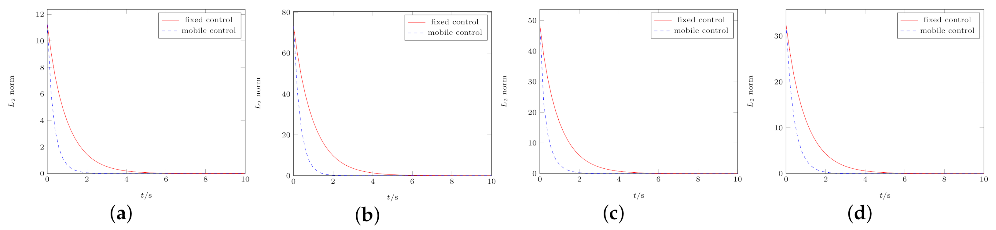
The control forces of mobile sensor–actuator have been designed by utilizing mobile sensor–actuator networks and Lyapunov functional technology, which have enhanced the estimators performance and made the state of estimation error systems converge to zero faster than that of fixed sensor–actuator networks.

The remainder of this paper is arranged as follows. The problem formulation under consideration is described, and the state estimators of delayed DPSs with missing measurements are designed in Section 2, along with some practical assumptions, useful definitions, and other detailed expression. In Section 3, we give the guidance policy of moving sensor–actuator pairs and, by utilizing Lyapunov functional technology, the operator semigroup approach, and stochastic analysis method, the control forces of mobile sensors–actuators are established and the estimation error systems are proved to be globally asymptotically stable in the mean square sense. Numerical simulation experiments are shown to illustrate the effectiveness of the estimation scheme in Section 4. Eventually, we come to a conclusion in Section 5.

2. Problem Formulation and Estimator Design

2.1. Problem Formulation and Preliminaries

This class of distributed parameter systems with time-delay under research is described by the n-input, n-output partial differential equations in one spatial dimension

$$\begin{array}{cc}\hfill \frac{\partial x(t,z)}{\partial t}=& a_1\frac{{\partial }^{2}x(t,z)}{\partial z^2}-a_{2}x(t,z)+a_{3}x(t-\tau \left(t\right),z)+\sum _{i=1}^{n}b(z;{\theta }_i^{\mathrm{a}}\left(t\right))u_i\left(t\right),\hfill \\ \hfill & (t,z)\in (0,+\infty )\times \Omega .\hfill \end{array}$$

(1)

$$\begin{array}{c}\hfill y\left(t\right)=\left[\begin{array}{c}{y}_1\left(t\right)\\ y_2\left(t\right)\\ ⋮\\ y_n\left(t\right)\end{array}\right]=\left[\begin{array}{c}{r}_1\left(t\right){\int }_0^{ϵ}c(z;{\theta }_1^{\mathrm{s}}\left(t\right))x(t,z)\mathrm{d}z\\ r_2\left(t\right){\int }_0^{ϵ}c(z;{\theta }_2^{\mathrm{s}}\left(t\right))x(t,z)\mathrm{d}z\\ ⋮\\ r_n\left(t\right){\int }_0^{ϵ}c(z;{\theta }_n^{\mathrm{s}}\left(t\right))x(t,z)\mathrm{d}z\end{array}\right],\end{array}$$

(2)

subject to Dirichlet boundary conditions

$$\begin{array}{c}\hfill x(t,0)=x(t,ϵ)=0,t\ge 0,\end{array}$$

(3)

and the initial condition

$$\begin{array}{c}\hfill x(t,z)=\phi (t,z),(t,z)\in [-\tau ,0]\times \Omega ,\end{array}$$

(4)

where the variables appearing in this paper are discussed in the real range $\mathbb{R}$. Suppose that there are n sensors and n actuators in the above model, $i=1,2,\cdots n$, $x(t,z)\in \mathbb{R}$ denotes the state which is transformed with time t and position $z,t\ge 0$, $z\in \Omega =[0,ϵ]$, and $ϵ>0$ means the upper boundary of a spatial region. $b(z;{\theta }_i^{\mathrm{a}}\left(t\right))$ is the bounded and known distribution function of the ith mobile actuator, and ${\theta }_i^a\left(t\right)\in \Omega$ indicates the time varying centroid of the ith mobile actuator. The known and bounded function $c(z;{\theta }_i^{\mathrm{s}}\left(t\right))$ depicts the spatial distribution of the ith mobile sensor, and ${\theta }_i^{\mathrm{s}}\left(t\right)\in \Omega$ is the spatial position of the ith mobile sensor. $\tau \left(t\right)$ is the time-varying delay, which satisfies that the boundedness $0\le \tau \left(t\right)\le \tau$ and the differentiability $\dot{\tau }\left(t\right)\le \eta <1$, $\tau ,\eta$ are positive constants, and $\phi (t,z)$ is a suitable smooth function. The positive constants $a_1,a_2,a_3$ describe diffusion coefficient, reaction coefficient and state delay coefficient, respectively. $r_i\left(t\right)$ stands for a random variable which values 0 or 1, $u_i\left(t\right)$ denotes the control input sign of this system. $y\left(t\right)$ represents the measurement outputs of mobile sensors, which is known on the condition that the sensors work well without missing measurements. However, $x(t,z)$ is unknown when the sensors give missing measurements, and thus it should be estimated.

Remark 1.

In the above systems, the state estimation for this delayed DPSs is different from the existed results in [44,47], which have not considered the time-delay in the DPSs. Therefore, the proposed estimation method in this paper is based on a new kind of DPS.

Remark 2.

In the above systems, $r_i\left(t\right)=0$ denotes that the measurement data of the ith sensor occurs missing, and $r_i\left(t\right)=1$ represents that the measurement data has been obtained without loss.

The first question under consideration in this article is to design state estimators which can approximate the original system state while occurring missing measurements. Therefore, we make the following assumptions aiming to address the problem simply.

Assumption 1.

We suppose that one sensor and one actuator in the mobile sensor–actuator networks are collocated into a same device, which is denoted as ${\theta }_i^{\mathrm{a}}\left(t\right)={\theta }_i^{\mathrm{s}}\left(t\right)={\theta }_i\left(t\right)$, the spatial distribution functions $b(z;{\theta }_i^{\mathrm{a}}\left(t\right))$ and $c(z;{\theta }_i^{\mathrm{s}}\left(t\right))$ are given by

$$\begin{array}{cc}\hfill b(z;{\theta }_i\left(t\right))& =c(z;{\theta }_i\left(t\right))\hfill \\ \hfill & =\left\{\begin{array}{cc}1,\hfill & z\in [{\theta }_i\left(t\right)-\epsilon ,{\theta }_i\left(t\right)+\epsilon ],\hfill \\ 0,\hfill & \mathrm{otherwise},\hfill \end{array}\right.\hfill \\ \hfill & =H({\theta }_i\left(t\right)-\epsilon )-H({\theta }_i\left(t\right)+\epsilon )),\hfill \end{array}$$

for $t>0,i=1,2,\cdots ,n$, and where $H({\theta }_i\left(t\right)-\epsilon )$ and $H({\theta }_i\left(t\right)+\epsilon )$ stand for the Heaviside step function, and $\epsilon >0$ denotes the effect radius of an actuator.

Remark 3.

There are two structures of sensors/actuators: one of the structures is non-collocated, which means that the sensor/actuator is divided into two parts, such as in [48] which defined that ${\theta }_i^{\mathrm{a}}\left(t\right)\ne {\theta }_i^{\mathrm{s}}\left(t\right)$ and $b(z;{\theta }_i^{\mathrm{a}}\left(t\right))\ne c(z;{\theta }_i^{\mathrm{s}}\left(t\right))$. However, according to the engineering application background of multi-agents in AI technology, we reasonably suppose that one sensor and one actuator in the mobile sensor–actuator networks are integrated into the same device, and in order to facilitate the presentation of this paper, the agent is represented for collocated sensor–actuator pairs.

Assumption 2.

In mobile agent networks, we assume that each agent is equipped with an estimator, when one agent has a missing measurement, the estimator needs to use the data of its surrounding agents to estimate. The communication energy consumption is depended on the number of its surrounding agents and the distance between them. The dynamic set of neighbor agents about the ith agent is $N_i\left(t\right)=\left\{j\right||{\theta }_i\left(t\right)-{\theta }_j\left(t\right)|<R,j\ne i,i,j\in \{1,2,\cdots n\}\}$, and the distance between any two agents should be confined to $|{\theta }_i\left(t\right)-{\theta }_j\left(t\right)|>(2r+\varrho )$ so as to avoid the mobile agents colliding together, where r is the shape radius of agent itself, ϱ indicates the minimum safe distance, and R is the maximum communication distance between the ith agent and others.

Remark 4.

In the paper [40,49], the neighbor set of the ith estimator was defined as $N_i=\left\{j\right||{\theta }_i-{\theta }_j|<R,i\ne j,i,j\in \{1,2,\cdots n\}\}$, R is the communication radius which had ignored the minimum distance. In the paper [50], the team discussed the distance between two agents in order to realize collision avoidance and gave $N_i=\left\{j\right||{\theta }_i-{\theta }_j|>2r,i\ne j,i,j\in \{1,2,\cdots n\}\}$, where r is the safety radius of each agent. In this work, we propose the dynamic estimator set of the ith agent $N_i\left(t\right)=\left\{j\right||{\theta }_i\left(t\right)-{\theta }_j\left(t\right)|<R,j\ne i,i,j\in \{1,2,\cdots n\}\}$ which subjects to $|{\theta }_i\left(t\right)-{\theta }_j\left(t\right)|>(2r+\varrho )$. Both the minimum anti-collision distance and the maximum communication distance are considered, which is more reasonable.

Assumption 3.

Considering the dynamic behavior of mobile agents, the motion equation of mobile agents is established on the basis of the Newton’s second law of motion, which is extended as

$$\begin{array}{c}\hfill \left\{\begin{array}{c}{f}_i\left(t\right)=m_i{\ddot{\theta }}_i\left(t\right)+d_i{\dot{\theta }}_i\left(t\right)+{\kappa }_i{\theta }_i\left(t\right),\hfill \\ {\theta }_i\left(0\right)={\theta }_{i0},{\dot{\theta }}_i\left(0\right)=0,i=1,2,\cdots ,n,\hfill \end{array}\right.\end{array}$$

where $m_i$ and ${\theta }_{i0}$ represent the mass and initial position of the ith agent, respectively. ${\dot{\theta }}_i\left(0\right)$, and ${\ddot{\theta }}_i\left(t\right)$, $f_i\left(t\right)$, respectively, describe the initial velocity, acceleration, and control force. $d_i\left(t\right)<0$ denotes the agent friction coefficient, and ${\kappa }_i\ge 0$ stands for the elastic coefficient.

Assumption 4.

In an appropriate sense, the missing measurements occur due to sensor failure or communication fault, which can be described by a random phenomenon. The stochastic variable $r_i\left(t\right)$ is a white noise sequence, which obeys a Bernoulli distribution and satisfies the following distribution:

$$\begin{array}{c}\hfill \left\{\begin{array}{c}\mathrm{Prob}\left\{r_i\left(t\right)=1\right\}=\mathbb{E}\left[r_i\left(t\right)\right]=q_i,\hfill \\ \mathrm{Prob}\left\{r_i\left(t\right)=0\right\}=1-\mathbb{E}\left[r_i\left(t\right)\right]=1-q_i,\hfill \end{array}\right.\end{array}$$

(5)

for $t>0,i=1,2,\cdots ,n$, where $q_i\in (0,1]$ is a known positive constant, and $\mathrm{Prob}\{·\}$ denotes probability. If the stochastic variables are independent, the distribution (5) can be given by

$$\begin{array}{c}\hfill \left\{\begin{array}{c}\mathbb{E}\left[r_i\left(t\right)-q_i\right]=0,\mathbb{E}\left[{(r_i\left(t\right)-q_i)}^2\right]=q_i(1-q_i),\hfill \\ \mathbb{E}\left[(r_i\left(t\right)-q_i)(r_j\left(t\right)-q_j)\right]=0,i\ne j,\hfill \end{array}\right.\end{array}$$

for $t>0,i=1,2,\cdots ,n,j=1,2,\cdots ,n$, where $\mathbb{E}[·]$ represents the mathematical expectation of a stochastic variable.

Remark 5.

From Assumption A1 and Assumption A4, and in the case of $r_i\left(t\right)\equiv 1$, the measurement outputs of system (2) are approximated by

$$\begin{array}{cc}\hfill y_i\left(t\right)& ={\int }_0^{ϵ}c(z;{\theta }_i\left(t\right))x(t,z)\mathrm{d}z\hfill \\ \hfill & ={\int }_{{\theta }_i\left(t\right)-\epsilon }^{{\theta }_i\left(t\right)+\epsilon }x(t,z)\mathrm{d}z\hfill \\ \hfill & \approx 2\epsilon \times \frac{x(t,{\theta }_i\left(t\right)-\epsilon )+x(t,{\theta }_i\left(t\right)+\epsilon )}{2}\hfill \\ \hfill & =\epsilon \times (x(t,{\theta }_i\left(t\right)-\epsilon )+x(t,{\theta }_i\left(t\right)+\epsilon ))\hfill \end{array}$$

2.2. System Evolution and Estimator Design

Combined with the method in the literature [38], we define $\mathcal{H}$ as a Hilbert space and $\mathcal{V}$ as a reflexive Banach space, ${\mathcal{V}}^{*}$ is the conjugate dual of $\mathcal{V}$. Let $\mathcal{H}$ be the inner product $\langle ·,·\rangle$ and induced norm $\parallel ·\parallel$; the induced norm of $\mathcal{V}$ and ${\mathcal{V}}^{*}$ are denoted by ${\parallel ·\parallel }_{\mathcal{V}}$ and ${\parallel ·\parallel }_{\mathcal{V}*}$, respectively. The relationship among $\mathcal{H}$, $\mathcal{V}$, and ${\mathcal{V}}^{*}$ is described by $\mathcal{V}\hookrightarrow \mathcal{H}\hookrightarrow {\mathcal{V}}^{*}$, the sign ↪ indicates both of them are embedding densely and continuously, in the sense that we can achieve $\parallel \varphi \parallel \le {c\parallel \varphi \parallel }_{\mathcal{V}}$, where $\varphi \in \mathcal{V}$, c is a positive constant. Additionally, the notation $\langle ·,·\rangle$ is also utilized to represent the duality pairing relationship between $\mathcal{V}$ and ${\mathcal{V}}^{*}$.

Utilizing the operator semigroup approach, the PDE (1) and (2) can be written as evolution equations abstractly in the Hilbert space:

$$\begin{array}{c}\hfill \left\{\begin{array}{c}\dot{x}\left(t\right)={\mathcal{A}}_{1}x\left(t\right)-{\mathcal{A}}_{2}x\left(t\right)+{\mathcal{A}}_{3}x(t-\tau \left(t\right))+\mathcal{B}\left(\theta \left(t\right)\right)u\left(t\right)\hfill \\ y\left(t\right)=\mathcal{R}\left(t\right)\mathcal{C}\left(\theta \right(t\left)\right)x\left(t\right),t>0,\hfill \end{array}\right.\end{array}$$

(6)

where ${\mathcal{A}}_1$ is a second-order operator given in [38]

$$\begin{array}{c}\hfill {\mathcal{A}}_1\varphi =a_1\frac{{\partial }^2\varphi }{\partial z^2},a_1>0,\varphi \in \mathrm{Dom}\left({\mathcal{A}}_1\right),\end{array}$$

where $\mathrm{Dom}\left({\mathcal{A}}_1\right)=\{\psi \in L_2\left(\Omega \right)|\psi ,{\psi }^{\prime }$ absolutely continuous, ${\psi }^{\prime \prime }\in L_2\left(\Omega \right)$ and $\psi \left(0\right)=\psi \left(l\right)=0\}$, which with boundedness $\left|〈{\mathcal{A}}_1\varphi ,\phi 〉\right|\le \alpha ∥\varphi ∥∥\phi ∥$, coercivity $〈-{\mathcal{A}}_1\varphi ,\varphi 〉\ge \beta {∥\varphi ∥}^2$, and symmetry $〈{\mathcal{A}}_1\varphi ,\phi 〉=〈\varphi ,{\mathcal{A}}_1\phi 〉$, for $\varphi ,\phi \in \mathcal{V}$, $\alpha >0$ and $\beta >0$. Both of ${\mathcal{A}}_2$, ${\mathcal{A}}_3$ are bounded operator, and $\mathcal{R}\left(t\right)=\mathrm{diag}(r_1\left(t\right),r_2\left(t\right),\cdots r_n\left(t\right))$.

$\mathcal{B}\left(\theta \right(t\left)\right)$ is the input operator defined as

$$\begin{array}{cc}\hfill \mathcal{B}\left(\theta \right(t\left)\right)u\left(t\right)& =[{\mathcal{B}}_1\left({\theta }_1\left(t\right)\right)\cdots {\mathcal{B}}_n\left({\theta }_n\left(t\right)\right)]\left[\begin{array}{c}{u}_1\left(t\right)\\ \cdots \\ u_n\left(t\right)\end{array}\right],\langle {\mathcal{B}}_i\left({\theta }_i\left(t\right)\right)u_i\left(t\right),\varphi \rangle \hfill \\ \hfill & ={\int }_0^{ϵ}b(z;{\theta }_i\left(t\right))\varphi \left(z\right)u_i\left(t\right)\mathrm{d}z.\hfill \end{array}$$

$\mathcal{C}\left(\theta \right(t\left)\right)$ denotes the output operator described by

$$\begin{array}{c}\hfill \langle \mathcal{C}\left(\theta \left(t\right)\right)\varphi ,\phi \rangle =\left[\begin{array}{c}\langle {\mathcal{C}}_1\left({\theta }_1\left(t\right)\right)\varphi ,\phi \rangle \\ \cdots \\ \langle {\mathcal{C}}_n\left({\theta }_n\left(t\right)\right)\varphi ,\phi \rangle \end{array}\right],\langle {\mathcal{C}}_i\left({\theta }_i\left(t\right)\right)\varphi ,\phi \rangle ={\int }_0^{ϵ}c(z;{\theta }_i\left(t\right))\varphi \left(z\right)\phi \left(z\right)\mathrm{d}z.\end{array}$$

Based on the PDE system (1), (2), and Assumption A2, when the missing measurement occurs in the ith agent, the corresponding state estimator is excogitated as

$$\begin{array}{cc}\hfill \frac{\partial {\widehat{x}}_i(t,z)}{\partial t}=& a_1\frac{{\partial }^2{\widehat{x}}_i(t,z)}{\partial z^2}-a_2{\widehat{x}}_i(t,z)+a_3{\widehat{x}}_i(t-\tau \left(t\right),z)+k_i(y_i\left(t\right)-q_i{\widehat{y}}_i\left(t\right))\hfill \\ \hfill & -l_i\sum _{j\in N_i\left(t\right)}({\widehat{x}}_i(t,z)-{\widehat{x}}_j(t,z))+\sum _{i=1}^{n}b(z;{\theta }_i^{\mathrm{a}}\left(t\right))u_i\left(t\right),i=1,2,\cdots ,n,\hfill \end{array}$$

(7)

where ${\widehat{x}}_i(t,z)$ indicates the estimation of $x(t,z)$ about the ith estimator, $l_i>0$ denotes the estimator gain, $k_i>0$ represents the consistency gain, and ${\widehat{y}}_i\left(t\right)={\mathcal{C}}_i{\widehat{x}}_i\left(t\right)$.

Remark 6.

The new designed distributed estimators are superior to the centralized estimator, and there are two disadvantages of the centralized estimator: one is that the centralized estimator usually utilizes all the system states to make estimation which results in a large computing capacity, and the other is that the system only designs one estimator; the estimator cannot work well when it occurs faults. Compared with the centralized estimator, we design a number of distributed estimators according to the system, which can reduce the computation and keep working when other estimators break down.

Adapting a similar conduct scheme to (6), the estimator Equation (7) can also be abstractly written as evolution equations

$$\begin{array}{cc}\hfill {\dot{\widehat{x}}}_i\left(t\right)=& {\mathcal{A}}_1{\widehat{x}}_i\left(t\right)-{\mathcal{A}}_2{\widehat{x}}_i\left(t\right)+{\mathcal{A}}_3{\widehat{x}}_i(t-\tau \left(t\right))+{\Gamma }_i(y_i\left(t\right)-q_i{\mathcal{C}}_i{\widehat{x}}_i\left(t\right))\hfill \\ \hfill & -L_i\sum _{j\in N_i\left(t\right)}({\widehat{x}}_i\left(t\right)-{\widehat{x}}_j\left(t\right))+\mathcal{B}\left(\theta \left(t\right)\right)u\left(t\right),i=1,2,\cdots ,n,\hfill \end{array}$$

where ${\widehat{x}}_i\left(0\right)={\widehat{x}}_{i0}\ne x\left(0\right)$, ${\Gamma }_i=k_i{\mathcal{C}}_i^{*}$ denotes the gain operator of the ith estimator, and $L_i$ is the consensus operator. Here, we define $e_i\left(t\right)=x\left(t\right)-{\widehat{x}}_i\left(t\right)$, and the estimation error system equations are achieved by

$$\begin{array}{c}\hfill {\dot{e}}_i\left(t\right)={\mathcal{A}}_1{e}_i\left(t\right)-{\mathcal{A}}_2{e}_i\left(t\right)+{\mathcal{A}}_3{e}_i(t-\tau \left(t\right))-k_i{\mathcal{C}}_i^{*}(y_i\left(t\right)-q_i{\mathcal{C}}_i{\widehat{x}}_i\left(t\right))+L_i\sum _{j\in N_i\left(t\right)}(e_j\left(t\right)-e_i\left(t\right)),\end{array}$$

(8)

$-k_i{\mathcal{C}}_i^{*}(y_i\left(t\right)-q_i{\mathcal{C}}_i{\widehat{x}}_i\left(t\right))$ in (8) can be calculated by

$$\begin{array}{cc}\hfill -k_i{\mathcal{C}}_i^{*}(y_i\left(t\right)-q_i{\mathcal{C}}_i{\widehat{x}}_i\left(t\right))=& -k_i{\mathcal{C}}_i^{*}{r}_i\left(t\right){\mathcal{C}}_{i}x\left(t\right)+k_i{\mathcal{C}}_i^{*}{q}_i{\mathcal{C}}_i{\widehat{x}}_i\left(t\right)\hfill \\ \hfill =& -k_i{\mathcal{C}}_i^{*}{r}_i\left(t\right){\mathcal{C}}_{i}x\left(t\right)+k_i{\mathcal{C}}_i^{*}{q}_i{\mathcal{C}}_{i}x\left(t\right)-k_i{\mathcal{C}}_i^{*}{q}_i{\mathcal{C}}_{i}x\left(t\right)+k_i{\mathcal{C}}_i^{*}{q}_i{\mathcal{C}}_i{\widehat{x}}_i\left(t\right)\hfill \\ \hfill =& -k_i{q}_i{\mathcal{C}}_i^{*}{\mathcal{C}}_i{e}_i\left(t\right)-k_i{\mathcal{C}}_i^{*}(r_i\left(t\right)-q_i){\mathcal{C}}_{i}x\left(t\right).\hfill \end{array}$$

(9)

Substituting (9) into (8) that we can get the estimation error system equations given by

$$\begin{array}{cc}\hfill {\dot{e}}_i\left(t\right)=& {\mathcal{A}}_1{e}_i\left(t\right)-{\mathcal{A}}_2{e}_i\left(t\right)+{\mathcal{A}}_3{e}_i(t-\tau \left(t\right))-k_i{q}_i{\mathcal{C}}_i^{*}{\mathcal{C}}_i{e}_i\left(t\right)\hfill \\ \hfill & -k_i{\mathcal{C}}_i^{*}(r_i\left(t\right)-q_i){\mathcal{C}}_i{x}_i\left(t\right)+L_i\sum _{j\in N_i\left(t\right)}(e_j\left(t\right)-e_i\left(t\right)),\hfill \end{array}$$

(10)

where $e_i\left(0\right)=x_i\left(0\right)-{\widehat{x}}_i\left(0\right)\ne 0$. Assuming ${\mathcal{A}}_{\mathrm{cl}}={\mathcal{A}}_1-{\mathcal{A}}_2-k_i{q}_i{\mathcal{C}}_i^{*}{\mathcal{C}}_i$, the estimation error system Equation (10) can be rewritten as

$$\begin{array}{c}\hfill {\dot{e}}_i\left(t\right)={\mathcal{A}}_{\mathrm{cl}}{e}_i\left(t\right)+{\mathcal{A}}_3{e}_i(t-\tau \left(t\right))-k_i{\mathcal{C}}_i^{*}(r_i\left(t\right)-q_i){\mathcal{C}}_{i}x\left(t\right)+L_i\sum _{j\in N_i\left(t\right)}(e_j\left(t\right)-e_i\left(t\right)).\end{array}$$

(11)

The output error equation is obtained by

$$\begin{array}{c}\hfill y_e\left(t\right)=\left[\begin{array}{c}{y}_{e1}\left(t\right)\\ \cdots \\ y_{en}\left(t\right)\end{array}\right]=\left[\begin{array}{c}{r}_1\left(t\right){\mathcal{C}}_1\left({\theta }_1\left(t\right)\right)(x\left(t\right)-{\widehat{x}}_1\left(t\right))\\ \cdots \\ r_n\left(t\right){\mathcal{C}}_n\left({\theta }_n\left(t\right)\right)(x\left(t\right)-{\widehat{x}}_n\left(t\right))\end{array}\right].\end{array}$$

The corresponding expectation of output error equation is

$$\begin{array}{c}\hfill \mathbb{E}\left[y_e\left(t\right)\right]=\left[\begin{array}{c}\mathbb{E}\left[y_{e1}\left(t\right)\right]\\ \cdots \\ \mathbb{E}\left[y_{en}\left(t\right)\right]\end{array}\right]=\left[\begin{array}{c}{q}_1{\mathcal{C}}_1{e}_1\left(t\right)\\ \cdots \\ q_n{\mathcal{C}}_n{e}_n\left(t\right)\end{array}\right].\end{array}$$

The second problem to be addressed is to design control forces of mobile agents by using the Lyapunov stability theorem, for the sake of making the estimation error systems (11) achieve globally asymptotically stable. Now, we make the following definitions.

Definition 1.

If the solution to estimation error systems with time-varying delay (11) satisfies [43]

$$\begin{array}{c}\hfill \underset{n\to \infty }{lim}\mathbb{E}[\parallel e_i\left(t\right){\parallel }^2]=0,t>0,i=1,2,\cdots ,n,\end{array}$$

the estimation error systems (11) are globally asymptotically stable in the mean square sense.

Definition 2.

Assume that the function $V\left(t\right)$ is a random process and the operator $\mathcal{L}$ conforms to

$$\begin{array}{c}\hfill \mathcal{L}V\left(t\right)=\underset{\Delta t\to 0^{+}}{lim}\frac{\mathbb{E}\left[V\right(t+\Delta t\left|t\right)-V\left(t\right)]}{\Delta t},t>0,\end{array}$$

$\mathcal{L}V\left(t\right)$ can be denoted as the infinitesimal generator.

Lemma 1.

(Barbalat Lemma) [51] f is a non-negative continuous function defined in $[0,+\infty )$, and if f is Lebesgue integrable and continuous on $[0,+\infty )$, $\underset{n\to \infty }{lim}f\left(t\right)=0$ is established.

Lemma 2.

The operator ${\mathcal{A}}_{\mathrm{cl}}$ has boundedness and coercivity along with the operator ${\mathcal{A}}_1$, which satisfies

$$\begin{array}{c}\hfill \left\{\begin{array}{c}\left|〈{\mathcal{A}}_{\mathrm{cl}}\varphi ,\phi 〉\right|\le (a_1+a_2{c}^2+c^{2}max\left(k_i{q}_i\right){\left|\mathcal{C}\right|}^2)∥\varphi ∥∥\phi ∥\hfill \\ 〈-{\mathcal{A}}_{\mathrm{cl}}\varphi ,\phi 〉\ge \left(\frac{a_1}{c^2}+a_2+min\left(k_i{q}_i\right){\left|\mathcal{C}\right|}^2\right){\left|\varphi \right|}^2.\hfill \end{array}\right.\end{array}$$

where $a_1,a_2,c,k_i,q_i$ are positive constants, and $\varphi ,\phi \in \mathcal{V}$.

Proof of Lemma 2 

We should give some supplementary knowledge before the proof, such as $\mathcal{H}$ is the Hilbert space, for $p\le q\in \mathbb{R}$, there has ${\int }_p^q{\left|x\right|}^2\mathrm{d}t<\infty$, and for $x,y\in \mathcal{H}$, $〈x,y〉={\int }_p^{q}x\overline{y}\mathrm{d}t$, $∥x∥={\left(〈x,x〉\right)}^{\frac{1}{2}}$, $〈·,·〉$ and $∥·∥$ denotes the inner product and induced norm, respectively.

Based on the properties of operator ${\mathcal{A}}_1$ [37], we know ${\mathcal{A}}_1$ has boundedness $\left|〈{\mathcal{A}}_1\varphi ,\phi 〉\right|\le \alpha ∥\varphi ∥∥\phi ∥$, coercivity $〈-{\mathcal{A}}_1\varphi ,\varphi 〉\ge \beta {∥\varphi ∥}^2$, and symmetry $〈{\mathcal{A}}_1\varphi ,\phi 〉=〈\varphi ,{\mathcal{A}}_1\phi 〉$, for $\varphi ,\phi \in \mathcal{V}$, $\alpha >0$ and $\beta >0$. Both of ${\mathcal{A}}_2$, ${\mathcal{A}}_3$ are bounded operator. Therefore, we have

$$\begin{array}{cc}\hfill |\langle {\mathcal{A}}_{\mathrm{cl}}\varphi ,\phi \rangle |=& |{\int }_0^{ϵ}\left(a_1\frac{{\mathrm{d}}^2\varphi \left(z\right)}{\mathrm{d}{z}^2}-a_2\varphi \left(z\right)\right)\phi \left(z\right)\mathrm{d}z|-|\langle k_i{q}_i{\mathcal{C}}_i^{*}{\mathcal{C}}_i\varphi ,\phi \rangle |\hfill \\ \hfill \le & a_1|{\int }_0^{ϵ}\frac{{\mathrm{d}}^2\varphi \left(z\right)}{\mathrm{d}{z}^2}\phi \left(z\right)\mathrm{d}z|+a_2|{\int }_0^{ϵ}\varphi \left(z\right)\phi \left(z\right)\mathrm{d}z|+|\langle k_i{q}_i{\mathcal{C}}_i\varphi ,{\mathcal{C}}_i\phi \rangle |\hfill \\ \hfill \le & a_1\sqrt{{\int }_0^{ϵ}{\left(\frac{\mathrm{d}\varphi \left(z\right)}{\mathrm{d}z}\right)}^2\mathrm{d}z}\sqrt{{\int }_0^{ϵ}{\left(\frac{\mathrm{d}\phi \left(z\right)}{\mathrm{d}z}\right)}^2\mathrm{d}z}+a_2\sqrt{{\int }_0^{ϵ}{\varphi }^2\left(z\right)\mathrm{d}z}\sqrt{{\int }_0^{ϵ}{\phi }^2\left(z\right)\mathrm{d}z}\hfill \\ \hfill & +max\left(k_i{q}_i\right){\left|\mathcal{C}\right|}^2\left|{\int }_0^{ϵ}\varphi \left(z\right)\phi \left(z\right)\mathrm{d}z\right|\hfill \\ \hfill =& a_1\parallel \varphi \parallel \parallel \phi \parallel +a_2\left|\varphi \right|\left|\phi \right|+max\left(k_i{q}_i\right){\left|\mathcal{C}\right|}^2\left|\varphi \right|\left|\phi \right|\hfill \\ \hfill \le & a_1\parallel \varphi \parallel \parallel \phi \parallel +a_2{c}^2\parallel \varphi \parallel \parallel \phi \parallel +c^{2}max\left(k_i{q}_i\right){\left|\mathcal{C}\right|}^2\parallel \varphi \parallel \parallel \phi \parallel \hfill \\ \hfill =& (a_1+a_2{c}^2+c^{2}max\left(k_i{q}_i\right)|\mathcal{C}{|}^2)\parallel \varphi \parallel \parallel \phi \parallel .\hfill \\ \hfill \langle -{\mathcal{A}}_{\mathrm{cl}}\varphi ,\varphi \rangle & ={\int }_0^{ϵ}\left(-a_1\frac{{\mathrm{d}}^2\varphi \left(z\right)}{\mathrm{d}{z}^2}+a_2\varphi \left(z\right)\right)\varphi \left(z\right)\mathrm{d}z+\left|\langle k_i{q}_i{\mathcal{C}}_i\varphi ,{\mathcal{C}}_i\varphi \rangle \right|\hfill \\ \hfill & \ge -a_1{\int }_0^{ϵ}\frac{{\mathrm{d}}^2\varphi \left(z\right)}{\mathrm{d}{z}^2}\varphi \left(z\right)\mathrm{d}z+a_2{\int }_0^{ϵ}\varphi \left(z\right)\varphi \left(z\right)\mathrm{d}z+min\left(k_i{q}_i\right){\left|\mathcal{C}\right|}^2{\int }_0^{ϵ}\varphi \left(z\right)\varphi \left(z\right)\mathrm{d}z\hfill \\ \hfill & =a_1{\parallel \varphi \parallel }^2+a_2{\left|\varphi \right|}^2+min\left(k_i{q}_i\right){\left|\mathcal{C}\right|}^2{\left|\varphi \right|}^2\hfill \\ \hfill & \ge \left(\frac{a_1}{c^2}+a_2+min\left(k_i{q}_i\right){\left|\mathcal{C}\right|}^2\right){\left|\varphi \right|}^2,\hfill \end{array}$$

the properties about boundedness and coercivity of operator ${\mathcal{A}}_{\mathrm{cl}}$ have been demonstrated. □

3. Main Results

In this section, the two questions raised above will be solved by using the Lyapunov stability method and stochastic analysis approach; the main results are given by the following theorem.

Theorem 1.

Consider this class of distributed parameter systems with time-varying delay described by (1)–(4), and the state estimators are excogitated as (7) when the agents exist missing measurements, the control force of the ith mobile agent is designed as

$$\begin{array}{c}\hfill {\displaystyle f_i\left(t\right)=-2{\lambda }_1{k}_i\mathbb{E}\left[\langle e_i\left(t\right),\frac{\partial {\mathcal{C}}_i^{*}}{\partial {\theta }_i\left(t\right)}{y}_{ei}\left(t\right)\rangle \right]+d_i{\dot{\theta }}_i\left(t\right)-\frac{({\lambda }_1{\rho }_{\mathrm{clb}}^2+{\lambda }_2)\sum _{i=1}^n\mathbb{E}\left[\parallel e_i\left(t\right){\parallel }^2\right]}{n{\dot{\theta }}_i\left(t\right)}.}\end{array}$$

(12)

$t>0,i=1,2,\cdots ,n$. If ${\dot{\theta }}_i\left(t\right)=0$, $f_i\left(t\right)$ can be dealt with

$$\begin{array}{cc}\hfill f_i\left(t\right)=& -2{\lambda }_1{k}_i\mathbb{E}\left[\langle e_i\left(t\right),\frac{\partial {\mathcal{C}}_i^{*}}{\partial {\theta }_i\left(t\right)}{y}_{ei}\left(t\right)\rangle \right]+d_i{\dot{\theta }}_i\left(t\right).\hfill \end{array}$$

(13)

Suppose that there exist some positive constants ${\lambda }_1,{\lambda }_2,{\lambda }_3,d_i$, which make the following inequalities be satisfied ${\lambda }_1{k}_i^2{\left|{\mathcal{C}}_i^{*}{\mathcal{C}}_i\right|}^2-{\lambda }_3<0$ and ${\lambda }_2\eta -{\lambda }_2+a_3{\lambda }_1<0$, the estimated error systems (11) are globally asymptotically stable in the mean square sense.

Proof of Theorem 1 

According to the Lyapunov function method [38,45,49], we choose the following Lyapunov functional candidate

$$\begin{array}{c}\hfill V\left(t\right)=V_1\left(t\right)+V_2\left(t\right)+V_3\left(t\right)+V_4\left(t\right),t>0,\end{array}$$

where $V\left(t\right)$ is a comprehensive Lyapunov function which involves $V_1\left(t\right),V_2\left(t\right),V_3\left(t\right),V_4\left(t\right)$. $V_1\left(t\right)$ is designed on the basis of Lemma 2. The purpose of $V_2\left(t\right)$ is to settle the time-delay problem in the DPSs, $V_3\left(t\right)$ considers the missing measurements, and $V_4\left(t\right)$ is to make an establishment for mobile forces on moving sensor/actuators.

$$\begin{array}{cc}\hfill & V_1\left(t\right)=-{\lambda }_1\sum _{i=1}^n\langle e_i\left(t\right),{\mathcal{A}}_{\mathrm{cl}}{e}_i\left(t\right)\rangle ,V_2\left(t\right)={\lambda }_2\sum _{i=1}^n{\int }_{t-\tau \left(t\right)}^t\langle e_i\left(s\right),e_i\left(s\right)\rangle \mathrm{d}s,\hfill \\ \hfill & V_3\left(t\right)=\sum _{i=1}^n{q}_i(1-q_i)\langle x\left(t\right),x\left(t\right)\rangle ,V_4\left(t\right)=\frac{1}{2}\sum _{i=1}^n(m_i{\left({\dot{\theta }}_i\left(t\right)\right)}^2+{\kappa }_i{\left({\theta }_i\left(t\right)\right)}^2).\hfill \end{array}$$

It is straightforward to find that $V_1\left(t\right)>0$ due to the coercivity of ${\mathcal{A}}_{\mathrm{cl}}$ in Lemma 1, where we obtain $V\left(t\right)>0$. Based on Definition 2, we have

$$\begin{array}{cc}\hfill \mathbb{E}\left[\mathcal{L}{V}_1\left(t\right)\right]=& -{\lambda }_1\sum _{i=1}^n\mathbb{E}\left[\langle {\dot{e}}_i\left(t\right),{\mathcal{A}}_{\mathrm{cl}}{e}_i\left(t\right)\rangle \right]-{\lambda }_1\sum _{i=1}^n\mathbb{E}\left[\langle e_i\left(t\right),{\dot{\mathcal{A}}}_{\mathrm{cl}}{e}_i\left(t\right)\rangle \right]-{\lambda }_1\sum _{i=1}^n\mathbb{E}\left[\langle e_i\left(t\right),{\mathcal{A}}_{\mathrm{cl}}{\dot{e}}_i\left(t\right)\rangle \right]\hfill \\ \hfill =& -2{\lambda }_1\sum _{i=1}^n\mathbb{E}\left[\langle {\dot{e}}_i\left(t\right),{\mathcal{A}}_{\mathrm{cl}}{e}_i\left(t\right)\rangle \right]+{\lambda }_1\sum _{i=1}^n\mathbb{E}\left[\langle e_i\left(t\right),\frac{\mathrm{d}}{\mathrm{d}t}\left(k_i{q}_i{\mathcal{C}}_i^{*}{\mathcal{C}}_i\right)e_i\left(t\right)\rangle \right]\hfill \\ \hfill =& -2{\lambda }_1\sum _{i=1}^n\mathbb{E}[\langle {\mathcal{A}}_{\mathrm{cl}}{e}_i\left(t\right)+{\mathcal{A}}_3{e}_i(t-\tau \left(t\right))-k_i{\mathcal{C}}_i^{*}(r_i\left(t\right)-q_i){\mathcal{C}}_{i}x\left(t\right)\hfill \\ \hfill & +L_i\sum _{j\in N_i\left(t\right)}(e_j\left(t\right)-e_i\left(t\right)),{\mathcal{A}}_{\mathrm{cl}}{e}_i\left(t\right)\rangle ]+{\lambda }_1\sum _{i=1}^n\mathbb{E}\left[\langle e_i\left(t\right),\frac{\mathrm{d}}{\mathrm{d}t}\left(k_i{q}_i{\mathcal{C}}_i^{*}{\mathcal{C}}_i\right)e_i\left(t\right)\rangle \right]\hfill \\ \hfill =& -2{\lambda }_1\sum _{i=1}^n\mathbb{E}\left[\langle {\mathcal{A}}_{\mathrm{cl}}{e}_i\left(t\right),{\mathcal{A}}_{\mathrm{cl}}{e}_i\left(t\right)\rangle \right]-2{\lambda }_1\sum _{i=1}^n\mathbb{E}\left[\langle {\mathcal{A}}_3{e}_i(t-\tau \left(t\right)),{\mathcal{A}}_{\mathrm{cl}}{e}_i\left(t\right)\rangle \right]\hfill \\ \hfill & +2{\lambda }_1\sum _{i=1}^n\mathbb{E}\left[\langle k_i{\mathcal{C}}_i^{*}(r_i\left(t\right)-q_i){\mathcal{C}}_{i}x\left(t\right),{\mathcal{A}}_{\mathrm{cl}}{e}_i\left(t\right)\rangle \right]\hfill \\ \hfill & -2{\lambda }_1{L}_i\sum _{i=1}^n\mathbb{E}\left[\langle \sum _{j\in N_i\left(t\right)}(e_j\left(t\right)-e_i\left(t\right)),{\mathcal{A}}_{\mathrm{cl}}{e}_i\left(t\right)\rangle \right]\hfill \\ \hfill & +{\lambda }_1\sum _{i=1}^n\mathbb{E}\left[\langle e_i\left(t\right),\frac{\mathrm{d}}{\mathrm{d}t}\left(k_i{q}_i{\mathcal{C}}_i^{*}{\mathcal{C}}_i\right)e_i\left(t\right)\rangle \right].\hfill \end{array}$$

It is necessary to separately solve the complex expression of $\mathbb{E}\left[\mathcal{L}{V}_1\left(t\right)\right]$, where

$$\begin{array}{cc}\hfill {\lambda }_1\sum _{i=1}^n\mathbb{E}\left[\langle e_i\left(t\right),\frac{\mathrm{d}}{\mathrm{d}t}\left(k_i{q}_i{\mathcal{C}}_i^{*}{\mathcal{C}}_i\right)e_i\left(t\right)\rangle \right]& =2{\lambda }_1\sum _{i=1}^n\mathbb{E}\left[\langle e_i\left(t\right),\frac{\mathrm{d}{\mathcal{C}}_i^{*}}{\mathrm{d}t}{k}_i{q}_i{\mathcal{C}}_i{e}_i\left(t\right)\rangle \right]\hfill \\ \hfill & =2{\lambda }_1\sum _{i=1}^n\mathbb{E}\left[\langle e_i\left(t\right),{\dot{\theta }}_i\left(t\right)\frac{\partial {\mathcal{C}}_i^{*}}{\partial {\theta }_i\left(t\right)}{k}_i{y}_{ei}\left(t\right)\rangle \right].\hfill \end{array}$$

(14)

Utilizing the internal machine inequality $2\langle x,y\rangle \le \langle x,x\rangle +\langle y,y\rangle$, we can obtain

$$\begin{array}{cc}\hfill -2{\lambda }_1\sum _{i=1}^n\mathbb{E}\left[\langle {\mathcal{A}}_3{e}_i(t-\tau \left(t\right)),{\mathcal{A}}_{\mathrm{cl}}{e}_i\left(t\right)\rangle \right]\le & {\lambda }_1\sum _{i=1}^n\mathbb{E}\left[\langle {\mathcal{A}}_3{e}_i(t-\tau \left(t\right)),{\mathcal{A}}_3{e}_i(t-\tau \left(t\right))\rangle \right]\hfill \\ \hfill & +{\lambda }_1\sum _{i=1}^n\mathbb{E}\left[\langle {\mathcal{A}}_{\mathrm{cl}}{e}_i\left(t\right),{\mathcal{A}}_{\mathrm{cl}}{e}_i\left(t\right)\rangle \right]\hfill \\ \hfill =& a_3{\lambda }_1\sum _{i=1}^n\mathbb{E}[\parallel e_i(t-\tau \left(t\right)){\parallel }^2]\hfill \\ \hfill & +{\lambda }_1\sum _{i=1}^n\mathbb{E}\left[\langle {\mathcal{A}}_{\mathrm{cl}}{e}_i\left(t\right),{\mathcal{A}}_{\mathrm{cl}}{e}_i\left(t\right)\rangle \right],\hfill \end{array}$$

(15)

and

$$\begin{array}{cc}\hfill & 2{\lambda }_1\sum _{i=1}^n\mathbb{E}\left[\langle k_i{\mathcal{C}}_i^{*}(r_i\left(t\right)-q_i){\mathcal{C}}_{i}x\left(t\right),{\mathcal{A}}_{\mathrm{cl}}{e}_i\left(t\right)\rangle \right]\hfill \\ \hfill & \le {\lambda }_1\sum _{i=1}^n\mathbb{E}\left[\langle k_i{\mathcal{C}}_i^{*}(r_i\left(t\right)-q_i){\mathcal{C}}_{i}x\left(t\right),k_i{\mathcal{C}}_i^{*}(r_i\left(t\right)-q_i){\mathcal{C}}_{i}x\left(t\right)\rangle \right]\hfill \\ \hfill & +{\lambda }_1\sum _{i=1}^n\mathbb{E}\left[\langle {\mathcal{A}}_{\mathrm{cl}}{e}_i\left(t\right),{\mathcal{A}}_{\mathrm{cl}}{e}_i\left(t\right)\rangle \right].\hfill \end{array}$$

(16)

By means of Assumption A4, one composition of (16) can be inferred

$$\begin{array}{cc}\hfill {\lambda }_1\sum _{i=1}^n\mathbb{E}\left[\langle k_i{\mathcal{C}}_i^{*}(r_i\left(t\right)-q_i){\mathcal{C}}_{i}x\left(t\right),k_i{\mathcal{C}}_i^{*}(r_i\left(t\right)-q_i){\mathcal{C}}_{i}x\left(t\right)\rangle \right]& ={\lambda }_1\sum _{i=1}^n\mathbb{E}\left[\parallel k_i{\mathcal{C}}_i^{*}(r_i\left(t\right)-q_i){\mathcal{C}}_{i}x\left(t\right){\parallel }^2\right]\hfill \\ \hfill & ={\lambda }_1\sum _{i=1}^n\mathbb{E}\left[k_i^2{q}_i(1-q_i){\parallel {\mathcal{C}}_i^{*}{\mathcal{C}}_{i}x\left(t\right)\parallel }^2\right]\hfill \\ \hfill & ={\lambda }_1\sum _{i=1}^n{k}_i^2{q}_i(1-q_i){\parallel {\mathcal{C}}_i^{*}{\mathcal{C}}_i{x}_i\left(t\right)\parallel }^2.\hfill \end{array}$$

(17)

Therefore, (16) is rewritten by

$$\begin{array}{cc}\hfill 2{\lambda }_1\sum _{i=1}^n\mathbb{E}\left[\langle k_i{\mathcal{C}}_i^{*}(r_i\left(t\right)-q_i){\mathcal{C}}_{i}x\left(t\right),{\mathcal{A}}_{\mathrm{cl}}{e}_i\left(t\right)\rangle \right]& \le {\lambda }_1\sum _{i=1}^n{k}_i^2{q}_i(1-q_i){\parallel {\mathcal{C}}_i^{*}{\mathcal{C}}_i{x}_i\left(t\right)\parallel }^2\hfill \\ \hfill & +{\lambda }_1\sum _{i=1}^n\mathbb{E}\left[\langle {\mathcal{A}}_{\mathrm{cl}}{e}_i\left(t\right),{\mathcal{A}}_{\mathrm{cl}}{e}_i\left(t\right)\rangle \right].\hfill \end{array}$$

(18)

Here, we define the $L_i=-{\mathcal{A}}_{\mathrm{cl}}^{-1}$ that can get

$$\begin{array}{c}\hfill -2{\lambda }_1{L}_i\sum _{i=1}^n\mathbb{E}\left[\langle \sum _{j\in N_i\left(t\right)}(e_j\left(t\right)-e_i\left(t\right)),{\mathcal{A}}_{\mathrm{cl}}{e}_i\left(t\right)\rangle \right]=-{\lambda }_1\sum _{i=1}^n\sum _{j\in N_i\left(t\right)}\mathbb{E}\left[\parallel e_i\left(t\right)-e_j\left(t\right){\parallel }^2\right].\end{array}$$

(19)

According to the above results (14)–(19), $\mathbb{E}\left[\mathcal{L}{V}_1\left(t\right)\right]$ is given by

$$\begin{array}{cc}\hfill \mathbb{E}\left[\mathcal{L}{V}_1\left(t\right)\right]\le & a_3\sum _{i=1}^n\mathbb{E}[\parallel e_i(t-\tau \left(t\right)){\parallel }^2]+{\lambda }_1\sum _{i=1}^n{k}_i^2{q}_i(1-q_i){\parallel {\mathcal{C}}_i^{*}{\mathcal{C}}_{i}x\left(t\right)\parallel }^2\hfill \\ \hfill & -{\lambda }_1\sum _{i=1}^n\sum _{j\in N_i}\mathbb{E}\left[\parallel e_i\left(t\right)-e_j\left(t\right){\parallel }^2\right]+2{\lambda }_1{k}_i\sum _{i=1}^n\mathbb{E}\left[\langle e_i\left(t\right),{\dot{\theta }}_i\left(t\right)\frac{\partial {\mathcal{C}}_i^{*}}{\partial {\theta }_i\left(t\right)}{y}_{ei}\left(t\right)\rangle \right].\hfill \end{array}$$

(20)

Meanwhile, $\mathbb{E}\left[\mathcal{L}{V}_2\left(t\right)\right]$ can be deduced by

$$\begin{array}{cc}\hfill \mathbb{E}\left[\mathcal{L}{V}_2\left(t\right)\right]& ={\lambda }_2\sum _{i=1}^n\mathbb{E}\left[\langle e_i\left(t\right),e_i\left(t\right)\rangle \right]-{\lambda }_2(1-\dot{\tau }\left(t\right))\sum _{i=1}^n\mathbb{E}\left[\langle e_i(t-\tau \left(t\right)),e_i(t-\tau \left(t\right))\rangle \right]\hfill \\ \hfill & ={\lambda }_2\sum _{i=1}^n\mathbb{E}\parallel e_i\left(t\right){\parallel }^2+({\lambda }_2\dot{\tau }\left(t\right)-{\lambda }_2)\sum _{i=1}^n\mathbb{E}\parallel e_i(t-\tau \left(t\right)){\parallel }^2\hfill \\ \hfill & \le {\lambda }_2\sum _{i=1}^n\mathbb{E}\parallel e_i\left(t\right){\parallel }^2+({\lambda }_2\eta -{\lambda }_2)\sum _{i=1}^n\mathbb{E}\parallel e_i(t-\tau \left(t\right)){\parallel }^2.\hfill \end{array}$$

(21)

Because of the infinitesimal production definition, we can obtain

$$\begin{array}{c}\hfill \mathbb{E}\left[\mathcal{L}{V}_3\left(t\right)\right]\le -{\lambda }_3\sum _{i=1}^n{q}_i(1-q_i){\parallel x\left(t\right)\parallel }^2,{\lambda }_3>0.\end{array}$$

(22)

Making use of Assumption A3, $\mathbb{E}\left[\mathcal{L}{V}_4\left(t\right)\right]$ is calculated by

$$\begin{array}{cc}\hfill \mathbb{E}\left[\mathcal{L}{V}_4\left(t\right)\right]& =\frac{1}{2}\sum _{i=1}^n(2m_i{\dot{\theta }}_i\left(t\right)\ddot{\theta }\left(t\right)+2{\kappa }_i{\theta }_i\left(t\right){\dot{\theta }}_i\left(t\right))\hfill \\ \hfill & =\sum _{i=1}^n{\dot{\theta }}_i\left(t\right)(m_i{\ddot{\theta }}_i\left(t\right)-d_i{\dot{\theta }}_i\left(t\right))\hfill \\ \hfill & =\sum _{i=1}^n{\dot{\theta }}_i\left(t\right)(f_i\left(t\right)-d_i{\dot{\theta }}_i\left(t\right)).\hfill \end{array}$$

(23)

Based on (20)–(23), we can get

$$\begin{array}{cc}\hfill \mathbb{E}\left[\mathcal{L}V\right(t\left)\right]\le & a_3{\lambda }_1\sum _{i=1}^n\mathbb{E}[\parallel e_i(t-\tau \left(t\right)){\parallel }^2]+{\lambda }_1\sum _{i=1}^n{k}_i^2{q}_i(1-q_i){\parallel {\mathcal{C}}_i^{*}{\mathcal{C}}_{i}x\left(t\right)\parallel }^2+{\lambda }_1\sum _{i=1}^n\mathbb{E}\left[\parallel {\mathcal{A}}_{\mathrm{cl}}{e}_i\left(t\right){\parallel }^2\right]\hfill \\ \hfill & -{\lambda }_1\sum _{i=1}^n\mathbb{E}\left[\parallel {\mathcal{A}}_{\mathrm{cl}}{e}_i\left(t\right){\parallel }^2\right]-{\lambda }_1\sum _{i=1}^n\sum _{j\in N_i\left(t\right)}\mathbb{E}\left[\parallel e_i\left(t\right)-e_j\left(t\right){\parallel }^2\right]\hfill \\ \hfill & +2{\lambda }_1{k}_i\sum _{i=1}^n\mathbb{E}\left[\langle e_i\left(t\right),{\dot{\theta }}_i\left(t\right)\frac{\partial {\mathcal{C}}_i^{*}}{\partial {\theta }_i\left(t\right)}{y}_{ei}\left(t\right)\rangle \right]+{\lambda }_2\sum _{i=1}^n\mathbb{E}[\parallel e_i\left(t\right){\parallel }^2]\hfill \\ \hfill & +({\lambda }_2\eta -{\lambda }_2)\sum _{i=1}^n\mathbb{E}[\parallel e_i(t-\tau \left(t\right)){\parallel }^2]-{\lambda }_3\sum _{i=1}^n{q}_i(1-q_i){\parallel x\left(t\right)\parallel }^2\hfill \\ \hfill & +\sum _{i=1}^n{\dot{\theta }}_i\left(t\right)(f_i\left(t\right)-d_i{\dot{\theta }}_i\left(t\right)).\hfill \end{array}$$

(24)

From Lemma 1, we can suppose ${\rho }_{\mathrm{cla}}^2\parallel e_i{\left(t\right)\parallel }^2\le \parallel {\mathcal{A}}_{\mathrm{cl}}{e}_i\left(t\right){\parallel }^2\le {\rho }_{\mathrm{clb}}^2{\parallel e_i\left(t\right)\parallel }^2$, ${\rho }_{\mathrm{clb}}>{\rho }_{\mathrm{cla}}>0$, (24) can be ulteriorly evolved by

$$\begin{array}{cc}\hfill \mathbb{E}\left[\mathcal{L}V\left(t\right)\right]\le & ({\lambda }_2\eta -{\lambda }_2+a_3{\lambda }_1)\sum _{i=1}^n\mathbb{E}[\parallel e_i(t-\tau \left(t\right)){\parallel }^2]+\sum _{i=1}^n({\lambda }_1{k}_i^2\parallel {\mathcal{C}}_i^{*}{\mathcal{C}}_i{\parallel }^2-{\lambda }_3)q_i(1-q_i){\parallel x\left(t\right)\parallel }^2\hfill \\ \hfill & -{\lambda }_1\sum _{i=1}^n\sum _{j\in N_i\left(t\right)}\mathbb{E}\left[\parallel e_i\left(t\right)-e_j\left(t\right){\parallel }^2\right]-{\lambda }_1{\rho }_{\mathrm{cla}}^2\sum _{i=1}^n\mathbb{E}\left[\parallel e_i\left(t\right){\parallel }^2\right]\hfill \\ \hfill & +\sum _{i=1}^n{\dot{\theta }}_i\left(t\right)(f_i\left(t\right)-d_i{\dot{\theta }}_i\left(t\right)+2{\lambda }_1{k}_i\sum _{i=1}^n\mathbb{E}\left[\langle e_i\left(t\right),\frac{\partial {\mathcal{C}}_i^{*}}{\partial {\theta }_i\left(t\right)}{y}_{ei}\left(t\right)\rangle \right]\hfill \\ \hfill & +\frac{({\lambda }_1{\rho }_{\mathrm{clb}}^2+{\lambda }_2)\sum _{i=1}^n\mathbb{E}\left[\parallel e_i\left(t\right){\parallel }^2\right]}{n{\dot{\theta }}_i\left(t\right)}).\hfill \end{array}$$

(25)

Assume there exist positive constants ${\lambda }_1,{\lambda }_2,{\lambda }_3,\eta ,k_i$ to make ${\lambda }_1{k}_i^2{\left|{\mathcal{C}}_i^{*}{\mathcal{C}}_i\right|}^2-{\lambda }_3<0$, ${\lambda }_2\eta -{\lambda }_2+a_3{\lambda }_1<0$ be established, $f_i\left(t\right)$ is presumed to (12) and (13), then (25) can be gained by

$$\begin{array}{c}\hfill \mathbb{E}\left[\mathcal{L}V\left(t\right)\right]\le -{\lambda }_1{\rho }_{\mathrm{cla}}^2\sum _{i=1}^n\mathbb{E}\left[\parallel e_i\left(t\right){\parallel }^2\right].\end{array}$$

(26)

From (26), we have

$$\begin{array}{c}\hfill \mathbb{E}\left[V(\infty )\right]-\mathbb{E}\left[V\left(0\right)\right]\le -{\lambda }_1{\rho }_{\mathrm{cla}}^2\sum _{i=1}^n\mathbb{E}\left[\parallel e_i\left(t\right){\parallel }^2\right].\end{array}$$

It can be indicated that ${\int }_0^{\infty }\mathbb{E}\left[\parallel e_i\left(t\right){\parallel }^2\right]\mathrm{d}\mathrm{t}<+\infty$ due to $V(\infty )\ge 0$ and $V\left(0\right)<+\infty$, and can be deduced that $\underset{n\to \infty }{lim}\mathbb{E}\left[\parallel e_i\left(t\right){\parallel }^2\right]=0$ on account of Barbalat Lemma 1. This completes the proof of Theorem 1; the estimation error systems (11) are globally asymptotically stable in the mean square sense. □

Remark 7.

In Theorem 1, the mobile control force $f_i\left(t\right)$ contains $-\frac{({\lambda }_1{\rho }_{\mathrm{clb}}^2+{\lambda }_2)\sum _{i=1}^n\mathbb{E}\left[\parallel e_i\left(t\right){\parallel }^2\right]}{n{\dot{\theta }}_i\left(t\right)}$, but $f_i\left(t\right)$ will be infinitely great when ${\dot{\theta }}_i\left(t\right)=0$. Therefore, $f_i\left(t\right)$ has been dealt with $f_i\left(t\right)=-2{\lambda }_1{k}_i\mathbb{E}\left[\langle e_i\left(t\right),\frac{\partial {\mathcal{C}}_i^{*}}{\partial {\theta }_i\left(t\right)}{y}_{ei}\left(t\right)\rangle \right]+d_i{\dot{\theta }}_i\left(t\right)$. In order to realize the simulation in Matlab, we define that $f_i\left(t\right)$ meets (13) when ${\dot{\theta }}_i\left(t\right)\le 0.001{\dot{\theta }}_i\left(0\right)$.

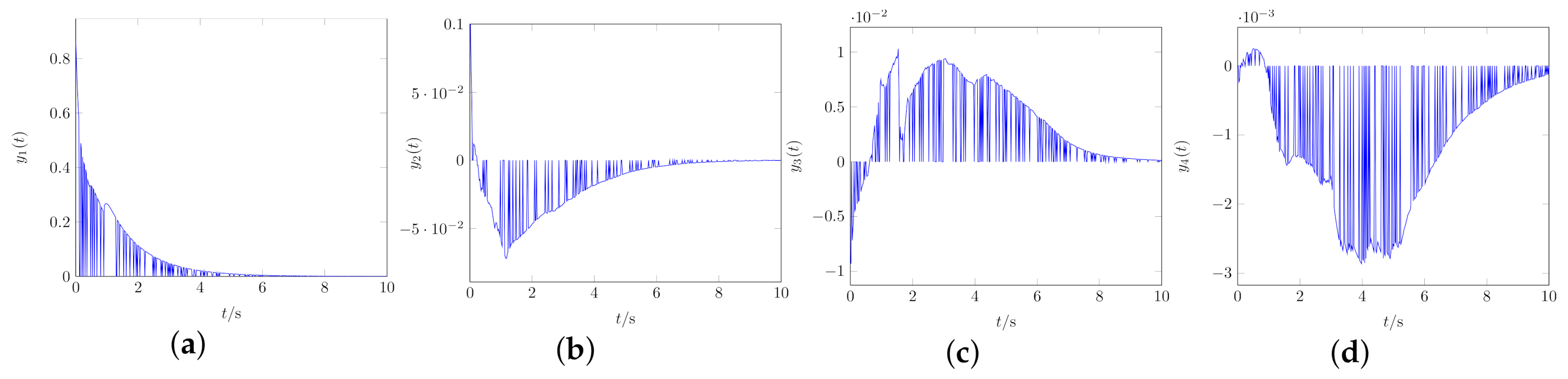
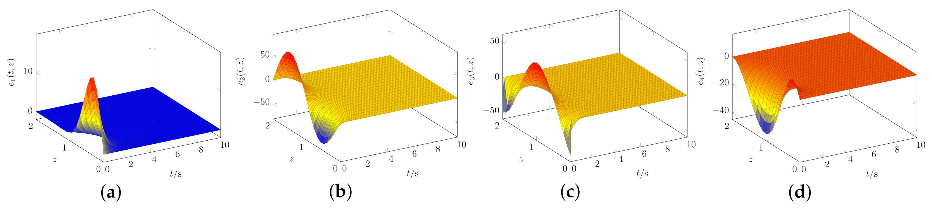
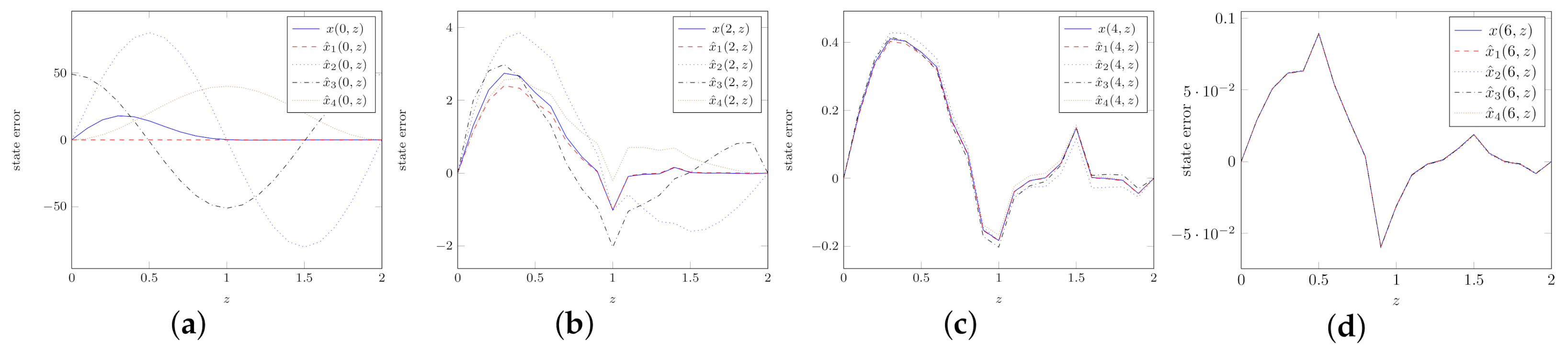
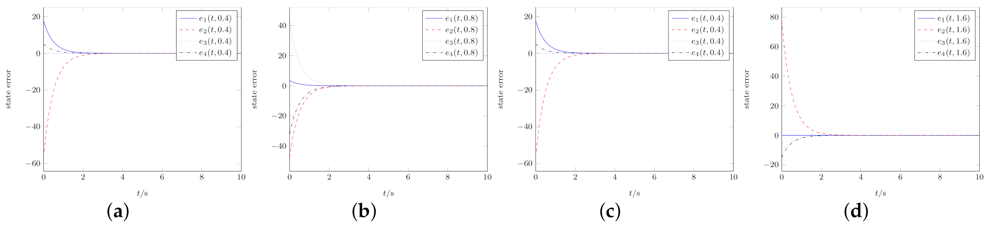
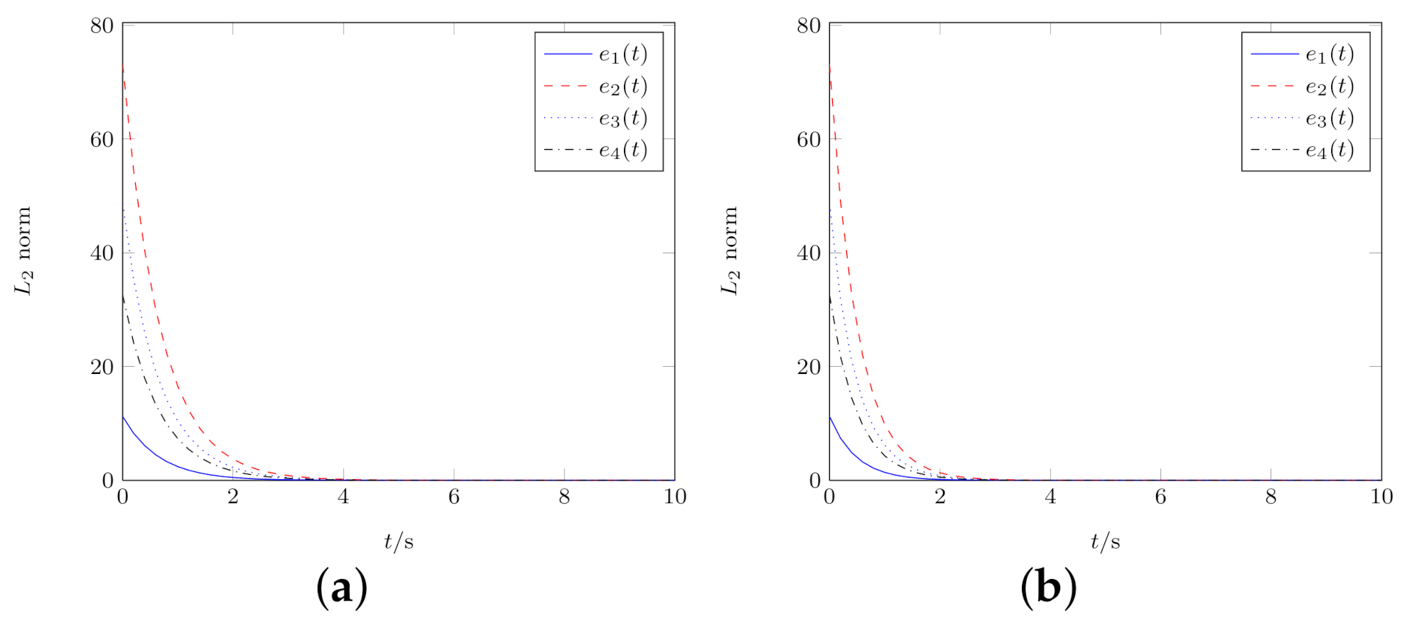
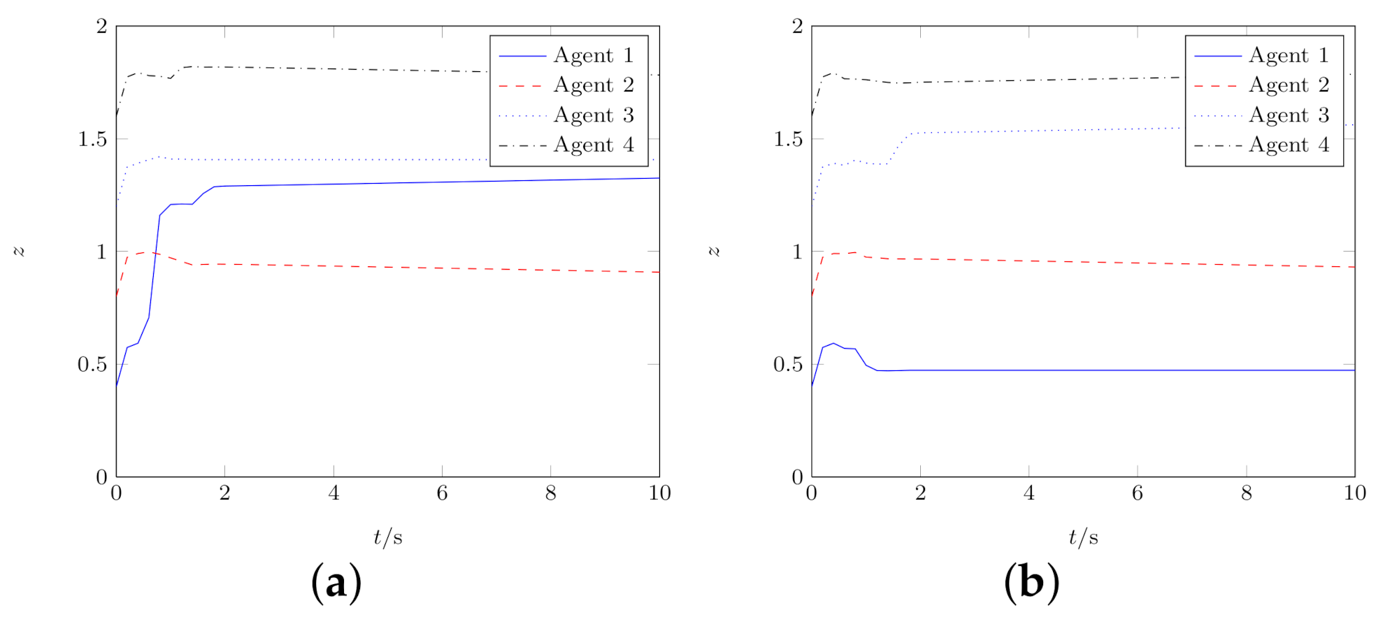
4. Numerical Results

In this section, we will illustrate the effectiveness of the control strategy proposed in this manuscript, which includes the estimators performances designed in (7), the asymptotically stability of estimation error systems (11), and the mobile control force (12) that acts on the dynamic agent.

We simulate the PDE systems (1)–(2) with initial condition $\phi (t,z)=30sin\left(\pi z\right)e^{-3z^2}(t+0.1),\tau =0.1,z\in [0,2]$, which satisfies Dirichlet boundary conditions $x(t,0)=x(t,2)=0$. The time-varying delay is $\tau \left(t\right)=0.1|sin(\pi t\left)\right|,\eta =0.2$, and the relevant parameters are defined as the diffusion coefficient $a_1=0.001$, the reaction coefficient $a_2=2$, and the state delay coefficient $a_3=1$.

The initial locations of four agents are set as ${\theta }_1\left(0\right)=0.4,{\theta }_2\left(0\right)=0.8,{\theta }_3\left(0\right)=1.2,{\theta }_4\left(0\right)=1.6$, and the maximum communication distance $R=0.6$, the shape radius $r=0.025$, the minimum safe distance $\varrho =0.1$, and the probability of agents appear missing measurement $1-q_i=0.2$. The initial conditions of four estimators are chosen as ${\widehat{x}}_1(0,z)=0$, ${\widehat{x}}_2(0,z)=80sin\left(\pi z\right)$, ${\widehat{x}}_3(0,z)=50cos\left(\pi z\right)-1$, ${\widehat{x}}_4(0,z)=20-20cos\left(\pi z\right)$.

Figure 1 shows the measurement outputs of four mobile agents with date missing probability $1-q_i\left(t\right)=0.2$. From Figure 1a–d, we can find the measurement outputs $y_i\left(t\right)$ have date loss because of the missing measurements.

Figure 2 describes the spatial states of four estimator under different initial conditions, where we discover that estimator 1 approximates the original system accurately because of the initial condition ${\widehat{x}}_1(0,z)=0$, other estimators have errors at the beginning duo to initial conditions with relatively large differences, but they can work well after 2–3 s.

In order to illustrate the effectiveness of estimators, the spatial states distribution of the actual system and four estimators at different times are shown in Figure 3, the evolution of estimation error systems states on four different locations are depicted in Figure 4.

We notice that the estimator includes the consistency component and the gain component, which has different effect on estimation error systems, so Figure 5 makes a comparative analysis about the evolution of state $L_2$ norms for estimation error systems with the consensus component and without the one, where we find the estimation error systems converge to zero fast with the consensus component.

Figure 6 depicts the trajectories of four agents under the control forces; the difference between Figure 6a,b is whether there exists a random missing measurement. It is obviously found that the agents collide together in a moment in Figure 6a; we deduce that the random missing measurement has affected the trajectory and meant that the agents cannot be controlled in the minimum safe distance.

The simulation results from Figure 1, Figure 2, Figure 3, Figure 4, Figure 5 and Figure 6 are obtained under mobile sensor–actuator networks, for the sake of comparing the effects between mobile control and fixed control, the $L_2$ norms of estimation error $e\left(t\right)$ are illustrated in Figure 7. Figure 7 shows the L2 norms of estimation error $e_1\left(t\right),e_2\left(t\right),e_3\left(t\right),e_4\left(t\right)$ under the fixed control and mobile control, although these four figures about Figure 7a–d are similar, the vertical coordinates of the four figures are different because the initial condition of ${\widehat{x}}_1(0,z),{\widehat{x}}_2(0,z),{\widehat{x}}_3(0,z),{\widehat{x}}_4(0,z)$ have made various error; however, it is easily observed from Figure 7 that the control strategy under mobile control is superior to the fixed control.

5. Conclusions

In this paper, the state estimation problem for a class of distributed parameter systems with time-varying delay over mobile sensor–actuator networks with missing measurements has been discussed and solved. The state estimation problem for a class of distributed parameter systems with time-varying delay over mobile sensor–actuator networks with missing measurements has been discussed and solved. One of the contributions is that we have projected a new kind of estimator to settle the estimation trouble which is based on the delayed DPSs, and the estimators are added with consistency component and gain component in order to approximate the system states effectively. The other contribution is that the designed estimators can restore the original system states when this delayed DPSs with stochastic missing measurements. In terms of proof of theory, we have constructed the estimation error systems by using the operator semigroup approach and the stochastic analysis method, and the estimation error systems are guaranteed to be globally asymptotically stable in the mean square via Lyapunov functional technology and mobile control forces. In the aspect of simulation verification, a large number of simulation experiments have been obtained to illustrate the effectiveness of this proposed estimation scheme, the simulation results indicate that the estimators have good estimation performance, and the states of estimation error systems converge to zero fast under mobile sensor–actuator network than that of fixed control.

Note that we consider the missing measurements as a random phenomenon when the sensors break down, which means that the data are lost with some probability. However, the original results of this paper can be extended to solve other problems such as the bad sensors give an abnormal data, only if we append a special mathematical function in the model.

References

1. Stafrace, S.K.; Antonopoulos, N. Military tactics in agent-based sinkhole attack detection for wireless ad hoc networks. Comput. Commun. 2010, 33, 619–638. [Google Scholar] [CrossRef]
2. Rehman, A.; Abbasi, A.Z.; Islam, N.; Shaikh, Z.A. A review of wireless sensors and networks applications in agriculture. Comput. Stand. Interfaces 2014, 36, 263–270. [Google Scholar] [CrossRef]
3. Aalsalem, M.Y.; Khan, W.Z.; Gharibi, W.; Khan, M.K.; Arshad, Q. Wireless Sensor Networks in oil and gas industry: Recent advances, taxonomy, requirements, and open challenges. J. Netw. Comput. Appl. 2018, 113, 87–97. [Google Scholar] [CrossRef]
4. Wu, H.F.; Xian, J.F.; Wang, J.; Khandge, S.; Mohapatra, P. Missing data recovery using reconstruction in ocean wireless sensor networks. Comput. Commun. 2018, 132, 1–9. [Google Scholar] [CrossRef]
5. Jenabzadeh, A.; Safarinejadian, B.; Binazadeh, T. Distributed tracking control of multiple nonholonomic mobile agents with input delay. Trans. Inst. Meas. Control 2018, 41, 805–815. [Google Scholar] [CrossRef]
6. Safarinejadian, B.; Kianpour, N.; Asad, M. State estimation in fractional-order systems with coloured measurement noise. Trans. Inst. Meas. Control 2017, 40, 1819–1835. [Google Scholar] [CrossRef]
7. Bounoua, W.; Benkara, A.B.; Kouadri, A.; Bakdi, A. Online monitoring scheme using principal component analysis through Kullback-Leibler divergence analysis technique for fault detection. Trans. Inst. Meas. Control 2019, 42, 1225–1238. [Google Scholar] [CrossRef]
8. Bu, X.H.; Tian, S.P.; Cui, L.Z.; Yang, J.Q. Stability and stabilization of 2-D Roesser systems with time-varying delays subject to missing measurements. Trans. Inst. Meas. Control 2017, 40, 1999–2010. [Google Scholar]
9. Ali, K.; Tahir, M. Maximum likelihood-based robust state estimation over a horizon length during measurement outliers. Trans. Inst. Meas. Control 2020. [Google Scholar] [CrossRef]
10. Lin, J.X.; Jiang, G.P.; Gao, Z.F.; Rong, L.N. State and input simultaneous estimation for discrete-time switched singular delay systems with missing measurements. Int. J. Robust Nonlinear Control 2016, 27, 2749–2772. [Google Scholar] [CrossRef]
11. Song, X.; Zheng, W.X. Linear estimation for discrete-time periodic systems with unknown measurement input and missing measurements. ISA Trans. 2019, 95, 164–172. [Google Scholar] [CrossRef] [PubMed]
12. Yang, R.; Li, L.; Su, X. Finite-region dissipative dynamic output feedback control for 2-D FM systems with missing measurements. Inf. Sci. 2020, 514, 1–14. [Google Scholar] [CrossRef]
13. Liu, W.; Tao, G.; Shen, C. Robust measurement fusion steady-state estimator design for multisensor networked systems with random two-step transmission delays and missing measurements. Math. Comput. Simul. 2021, 181, 242–283. [Google Scholar] [CrossRef]
14. Behrooz, H.A.; Boozarjomehry, R.B. Distributed and decentralized state estimation in gas networks as distributed parameter systems. ISA Trans. 2015, 58, 552–566. [Google Scholar] [CrossRef] [PubMed]
15. Wang, H.; Xue, A. Adaptive event-triggered H filtering for discrete-time delayed neural networks with randomly occurring missing measurements. Signal Process. 2018, 153, 221–230. [Google Scholar] [CrossRef]
16. Chen, X.; Zhao, S.; Liu, F. Identification of jump Markov autoregressive exogenous systems with missing measurements. J. Frankl. Inst. 2020, 357, 3498–3523. [Google Scholar] [CrossRef]
17. Zhang, J.; Gao, S.; Li, G.; Xia, J.; Qi, X.; Gao, B. Distributed recursive filtering for multi-sensor networked systems with multi-step sensor delays, missing measurements and correlated noise. Signal Process. 2021, 181, 107868. [Google Scholar] [CrossRef]
18. Liang, J.L.; Wang, Z.Z.; Liu, X.H. Distributed State Estimation for Discrete-Time Sensor Networks With Randomly Varying Nonlinearities and Missing Measurements. IEEE Trans. Neural Netw. 2011, 22, 486–496. [Google Scholar] [CrossRef] [Green Version]
19. Zhang, J.; Wang, Z.D.; Ding, D.R.; Liu, X.H. Hstate estimation for discrete-time delayed neural networks with randomly occurring quantizations and missing measurements. Neurocomputing 2015, 148, 388–396. [Google Scholar] [CrossRef]
20. Shu, H.S.; Zhang, S.J.; Shen, B.; Liu, Y. Unknown input and state estimation for linear discrete-time systems with missing measurements and correlated noises. Int. J. Gen. Syst. 2016, 45, 648–661. [Google Scholar] [CrossRef]
21. Wang, Z.G.; Chen, D.Y.; Du, J.H. Distributed variance-constrained robust filtering with randomly occurring nonlinearities and missing measurements over sensor networks. Neurocomputing 2019, 329, 397–406. [Google Scholar] [CrossRef]
22. Zhang, H.X.; Hu, J.; Liu, H.J.; Yu, X.Y.; Liu, F.Q. Recursive state estimation for time-varying complex networks subject to missing measurements and stochastic inner coupling under random access protocol. Neurocomputing 2019, 346, 48–57. [Google Scholar] [CrossRef]
23. Hu, J.; Wang, Z.; Liu, G.P.; Jia, C.; Williams, J. Event-triggered recursive state estimation for dynamical networks under randomly switching topologies and multiple missing measurements. Automatica 2020, 115, 108908. [Google Scholar] [CrossRef]
24. Ran, C.J.; Deng, Z.L. Robust fusion Kalman estimators for networked mixed uncertain systems with random one-step measurement delays, missing measurements, multiplicative noises and uncertain noise variances. Inf. Sci. 2020, 534, 27–52. [Google Scholar] [CrossRef]
25. Bolic, M.; Djuric, P.; Hong, S. Resampling algorithms and architectures for distributed particle filters. IEEE Trans. Signal Process. 2005, 53, 2442–2450. [Google Scholar] [CrossRef] [Green Version]
26. Read, J.; Achutegui, K.; Míguez, J. A distributed particle filter for nonlinear tracking in wireless sensor networks. Signal Process. 2014, 98, 121–134. [Google Scholar] [CrossRef]
27. Míguez, J.; Vázquez, M.A. A proof of uniform convergence over time for a distributed particle filter. Signal Process. 2016, 122, 152–163. [Google Scholar] [CrossRef] [Green Version]
28. Martino, L.; Elvira, V. Compressed Monte Carlo with application in particle filtering. Inf. Sci. 2021, 553, 331–352. [Google Scholar] [CrossRef]
29. Dai, X.S.; Tu, X.M.; Zhao, Y.; Tan, G.X.; Zhou, X.Y. Iterative learning control for MIMO parabolic partial difference systems with time delay. Adv. Differ. Equ. 2018, 2018, 344. [Google Scholar] [CrossRef]
30. Dai, X.S.; Mei, S.G.; Tian, S.P.; Yu, L. D-type iterative learning control for a class of parabolic partial difference systems. Trans. Inst. Meas. Control 2018, 40, 3105–3114. [Google Scholar] [CrossRef]
31. Dai, X.S.; Wang, C.; Tian, S.P.; Huang, Q.N. Consensus control via iterative learning for distributed parameter models multi-agent systems with time-delay. J. Frankl. Inst. 2019, 356, 5240–5259. [Google Scholar] [CrossRef]
32. Patan, M.; Uciński, D. Configuration of sensor network with uncertain location of nodes for parameter estimation in distributed parameter systems. IFAC Proc. Vol. 2009, 42, 31–36. [Google Scholar] [CrossRef]
33. Studener, S.; Habaieb, K.; Lohmann, B.; Wolf, R. Estimation of process parameters on a moving horizon for a class of distributed parameter systems. J. Process Control 2010, 20, 58–62. [Google Scholar] [CrossRef]
34. Cai, J.; Ferdowsi, H.; Sarangapani, J. Model-based fault detection, estimation, and prediction for a class of linear distributed parameter systems. Automatica 2016, 66, 122–131. [Google Scholar] [CrossRef] [Green Version]
35. Hu, W.; Wen, G.; Rahmani, A.; Yu, Y. Parameters estimation using mABC algorithm applied to distributed tracking control of unknown nonlinear fractional-order multi-agent systems. Commun. Nonlinear Sci. Numer. Simul. 2019, 79, 104933. [Google Scholar] [CrossRef]
36. Dash, M.; Panigrahi, T.; Sharma, R. Distributed parameter estimation of IIR system using diffusion particle swarm optimization algorithm. J. King Saud Univ. Eng. Sci. 2019, 31, 345–354. [Google Scholar] [CrossRef]
37. Demetriou, M.A.; Hussein, I.I. Estimation of spatially distributed processes using mobile spatially distributed sensor network. SIAM J. Control Optim. 2009, 48, 266–291. [Google Scholar] [CrossRef] [Green Version]
38. Demetriou, M.A. Guidance of Mobile Actuator-Plus-Sensor Networks for Improved Control and Estimation of Distributed Parameter Systems. IEEE Trans. Autom. Control 2010, 55, 1570–1584. [Google Scholar] [CrossRef]
39. Demetriou, M.A.; Ucinski, D. State estimation of spatially distributed processes using mobile sensing agents. In Proceedings of the 2011 American Control Conference, Orlando, FL, USA, 12–15 December 2011; IEEE: San Francisco, CA, USA, 2011; pp. 1770–1776. [Google Scholar]
40. Demetriou, M.A. Guidance of a moving sensor used in state estimation of a flexible beam. In Proceedings of the 53rd IEEE Conference on Decision and Control, Los Angeles, CA, USA, 15–17 December 2014; IEEE: Los Angeles, CA, USA, 2014; pp. 557–562. [Google Scholar]
41. Egorova, T.; Demetriou, M.A.; Gatsonis, N.A. Estimation of a gaseous release into the atmosphere using an unmanned aerial vehicle. In Proceedings of the 2015 European Control Conference, Linz, Austria, 15–17 July 2015; IEEE: Linz, Austria, 2015; pp. 873–878. [Google Scholar]
42. Mu, W.Y.; Cui, B.T.; Li, W.; Jiang, Z. Improving control and estimation for distributed parameter systems utilizing mobile actuator–sensor network. ISA Trans. 2014, 53, 1087–1095. [Google Scholar] [CrossRef] [PubMed]
43. Jiang, Z.X.; Cui, B.T. Estimation of spatially distributed processes using mobile sensor networks with missing measurements. Chin. Phys. B 2015, 24, 113–119. [Google Scholar] [CrossRef]
44. Jiang, Z.X.; Cui, B.T.; Lou, X.Y. Distributed consensus estimation for diffusion systems with missing measurements over sensor networks. Int. J. Syst. Sci. 2016, 47, 2753–2761. [Google Scholar] [CrossRef]
45. Zhang, J.Z.; Cui, B.T. Controlling a class of stochastic distributed parameter systems using mobile sensor-actuator networks with missing measurements. In Proceedings of the 2017 Chinese Automation Congress, Jinan, China, 20–22 October 2017; IEEE: Jinan, China, 2017; pp. 451–455. [Google Scholar]
46. Zhang, J.Z.; Cui, B.T. Mobile observation for distributed parameter system with moving boundary over mobile sensor networks. J. Control Decis. 2019, 1–18. [Google Scholar] [CrossRef]
47. Zhang, J.Z.; Lv, G.L.; Jiang, Z.X. State estimation for parabolic PDE system with moving boundary utilizing mobile sensor networks with missing measurements. In Proceedings of the 20th Chinese Control And Decision Conference, Hefei, China, 20–21 June 2020; IEEE: Hefei, China, 2020; pp. 2262–2267. [Google Scholar]
48. Zhang, J.Z.; Cui, B.T.; Zhuang, B. Improved control for distributed parameter systems with time-dependent spatial domains utilizing mobile sensor–actuator networks. Chin. Phys. B 2017, 26, 11–20. [Google Scholar] [CrossRef]
49. Jiang, Z.X.; Cui, B.T.; Lou, X.Y. Improved Control of Distributed Parameter Systems with Time-Varying Delay Based on Mobile Actuator-Sensor Networks. In Proceedings of the 19th World Congress of the International Federation of Automatic Control, Cape Town, South Africa, 24–29 August 2014; IEEE: Cape Town, South Africa, 2014; pp. 24–29. [Google Scholar]
50. Dai, L.; Cao, Q.; Xia, Y.; Gao, Y. Distributed MPC for formation of multi-agent systems with collision avoidance and obstacle avoidance. J. Frankl. Inst. 2017, 354, 2068–2085. [Google Scholar] [CrossRef]
51. Slotine, J.J.; Li, W.; Hall, P. Applied Nonlinear Control: United States Edition; Pearson Education Inc.: Prentice-Hall, NJ, USA, 1991. [Google Scholar]
Short Biography of Authors
Mathematics 09 00661 i001Huansen Fu received his B.S. degree in Electrical Engineering and Automation in 2006 and his M.S. degree in 2008 in Power Electronics and Power Drives from Jiangnan University, Wuxi, Jiangsu, China. He is currently pursuing the Ph.D. degree in Control Theory and Control Engineering from Jiangnan University, and he is currently an associate professor of Taizhou University, Taizhou, Jiangsu, China. His interests include distributed parameter systems, intelligent automation and application, process control.
Mathematics 09 00661 i002Baotong Cui received his Ph.D. degree in Control Theory and Control Engineering from the College of Automation Science and Engineering, South China University of Technology, in 2003. He was a post-doctoral fellow at Shanghai Jiaotong University from July 2003 to September 2005, and a visiting scholar at Department of Electrical and Computer Engineering, National University of Singapore from August 2007 to February 2008. He is now a professor in the School of IoT Engineering, Jiangnan University. His current research interests include systems analysis, stability theory, artificial neural networks and chaos synchronization.
Mathematics 09 00661 i003Bo Zhuang received his B.S. degree in Computer Science and Education and his M.S. degree in Computer Science and Technology from Shandong Normal University in 1999 and 2008, respectively. He received his Ph.D. degree in Control Theory and Control Engineering from School of IoT Engineering in 2019, Jiangnan University, Wuxi, Jiangsu, China. His current research interests include distributed parameter systems, and multi-agent systems.
Mathematics 09 00661 i004Jianzhong Zhang received the B.S. and M.S. degrees in Mathematics in 2005 and 2008 from Shandong University of Science and Technology, Tsingtao, Shandong, China, and the Ph.D. degree in Control Science and Engineering in 2019 from Jiangnan University, Wuxi, Jiangsu, China. He is currently a lecturer in School of Mathematics and Statistics, Taishan University. His current research interests include distributed parameter systems, networked control systems, mobile control and stability theory.
Figure 1. The outputs of four agents under stochastic measurement with date missing probability 1 q i ( t ) = 0.2 . (a) Output of agent 1. (b) Output of agent 2. (c) Output of agent 3. (d) Output of agent 4.
Mathematics 09 00661 g001
Figure 2. The spatial states of four estimators. (a) Spatial state of estimator 1. (b) Spatial state of estimator 2. (c) Spatial state of estimator 3. (d) Spatial state of estimator 4.
Mathematics 09 00661 g002
Figure 3. The spatial states distribution of the actual system and the four estimators at four different times. (a) t = 0 s. (b) t = 2 s. (c) t = 4 s. (d) t = 8 s.
Mathematics 09 00661 g003
Figure 4. The evolution of estimation error states on four different locations. (a) z = 0.4 . (b) z = 0.8 . (c) z = 1.2 . (d) z = 1.6 .
Mathematics 09 00661 g004
Figure 5. The evolution of state L 2 norms about estimation error system. (a) L 2 norm without consensus. (b) L 2 norm with consensus.
Mathematics 09 00661 g005
Figure 6. The trajectories of four mobile agents under different missing measurement probability. (a) 1 q i ( t ) = 0.2 . (b) 1 q i ( t ) = 0 .
Mathematics 09 00661 g006
Figure 7. The L 2 norms of estimation error e ( t ) under fixed control and mobile control. (a) L 2 norm of e 1 ( t ) . (b) L 2 norm of e 2 ( t ) . (c) L 2 norm of e 3 ( t ) . (d) L 2 norm of e 4 ( t ) .
Mathematics 09 00661 g007
Publisher’s Note: MDPI stays neutral with regard to jurisdictional claims in published maps and institutional affiliations.