1. Introduction
For humans, it does not take too much effort to tell apart trousers from a sweater or to recognize the outfit of a person. However, assigning features in an image to a certain category is still a hard problem to solve for computers [
1]. Images are captured everywhere. On Facebook alone, about 350 million images are uploaded every day [
2], and many of them contain fashion objects or apparel. With the continuously increasing amount of data, it is crucial to automatically extract information out of image data. Over the last decade, the progress to address these deep learning problems has been enormous. The latest common method to understand features in images is a model called a convolutional neural network (CNN), a subtype of neural networks [
3].
1.1. Problem Statement
It is a difficult task to find the most suitable architecture for the models’ classification purpose, and it often takes a lot of time and trials. In addition, these convolutional neural networks require big datasets, and despite the ever-increasing amount of image data, in real-world applications, it is often difficult to get access to image data if you are not a company like Facebook or Google. For this, researchers have introduced techniques like dropout regularity, data augmentation and transfer learning to make models more generalizable even when they are trained on a small dataset.
The existing literature mostly addresses the problem of recognizing and classifying product images in order to, for example, suggest similar products in online stores. However, the research for classifying human-worn fashion images is limited, and the rapidly growing e-commerce industry offers plenty of application scenarios for image classification. One of them is to automatically add links to social media posts that lead to an online shop with already predefined search criteria.
The goal of this research is to provide a successful approach for implementing an image classification model on a small dataset to extract features in fashion images. The results will show which methods and approaches are best suited for classifying fashion images and which techniques help to improve the generalization of small datasets.
1.2. Structure of the Work
This article begins with a brief insight into machine learning to provide a fundamental understanding of how machines learn. Next, neural networks are discussed. Here, it will first be described how single artificial neurons try to mimic biological neurons and how they process inputs to generate outputs, before networks that consist of thousands of neurons are explained. In the following subsections, it will be discussed how convolutional neural networks can be used for image classification, as well as how and when transfer learning should be applied. Furthermore, the most important types of layers and frameworks are explained.
The third section specifies the setup for the implementation phase and gives an overview of the most popular frameworks and libraries. In the fourth section, the public benchmark dataset Fashion MNIST and, in the course of this article, the created dataset are given.
In the fifth and sixth section, the different implementation approaches are described and implemented before being evaluated by their performance. Sections seven, eight and nine are meant to discuss, conclude and give an outlook on the article for further work.
1.3. Boundaries
This article attempts to examine the standard to automatically extract features in fashion images and aims to successfully implement an image classification model. The implemented image classifier shall be able to classify the input images into one of the following ten classes:
Bag;
Coat;
Dress;
Hat;
Pullover;
Shoes;
Shirt;
Suit;
Trouser;
T-shirt.
Furthermore, the color, pattern or brand of the clothes will not be considered in the classification and is not a part of this article.
2. Literature Review
This section provides the theoretical background necessary to understand the methods and approaches in the following sections. First, machine learning (ML) is described in general, with its most common types followed by the most relevant details of neural networks being given. Finally, it will be explained how these disciplines are combined in convolutional neural networks (CNNs) and what CNNs can achieve.
2.1. Machine Learning Types and Algorithms
Machine learning algorithms can be largely classified in two main types: supervised and unsupervised learning. The main difference between these two taxonomies is that with supervised learning, the algorithm is given labeled data with a known and correct output, whereas when it comes to unsupervised data, the output of the algorithm is unknown. This also explains the naming, as the labeling for the output vectors of the data requires a supervisor [
4].
Supervised learning is the most widely used ML form in practice and is most common for solving classification and regression problems. In classification, the model is required to learn a function which maps input vectors into one of several classes by looking at several input–output examples called training data [
5]. A typical supervised machine learning function looks as simple as the following:
where
Y is the predicted outcome,
f is an unknown function and
X represents the input data.
Classification again comes in two forms:
binary classification and
multiclass classification. If the classification consists of just two possible outcomes (zero or one), then it speaks of a binary classification. On the other hand, if there are more than two possible outcomes, it speaks of a multiclass classification [
6]. A regression problem is when the function tries to predict a continuous output variable, such as stocks or salaries [
7].
Unsupervised Learning is harder to implement, as the ML algorithm does not have a training set to learn from. Computers are presented with real-world data without the corresponding correct output values and must learn from that data on their own [
8]. Clustering is most often used for unsupervised learning and has the goal of discovering a structure or patterns by investigating similarities between the objects in the input data [
7].
2.2. Neural Networks for Image Classification
Neural networks have their origins in 1943, when Warren McCulloch and Walter Pitts published a paper on how neurons work and presented the first model of artificial neurons [
9]. This model could approximate the output as a weighted sum of the inputs that is passed through a threshold function [
6]. Between 1957 and 1958, Frank Rosenblatt’s research in neurobiology resulted in the invention of the perceptron, the oldest neural network that is still in use [
9]. In the 1970s, Marvin Minsky and Seymour Papert published the book Perceptrons, demonstrating all the concerning limitations, which diminished the interest in the field and led to some quiet years [
10]. In 1986, backpropagation was introduced by Rumelhart, Hinton and Williams [
11], which enabled it to fit models with hidden layers [
12]. This was marked as a breakthrough in neural network algorithms.
The fact that research in modern neural networks is mostly guided by mathematicians and engineers rather than biologists also shows that it is not the goal to perfectly model the brain, but to achieve statistical generalization through approximation function machines [
13].
2.2.1. Artificial Neurons
An artificial neuron is considered the basic element in an artificial neural network (ANN) [
14] and carries out the computational operations in the network. The way these neurons are interconnected constitutes the neural network [
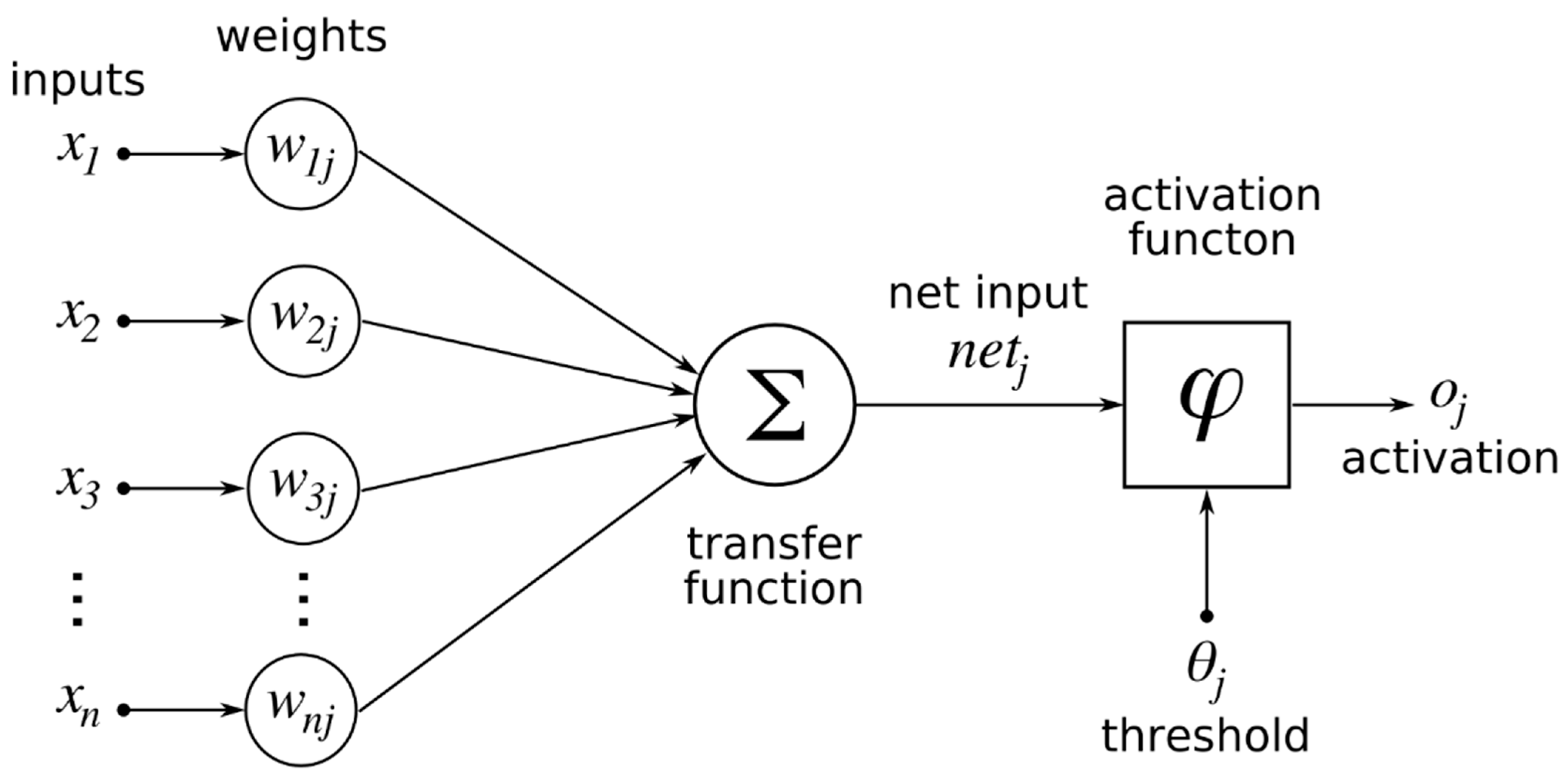
15]. In general, a neuron receives two or more inputs from other neurons, which are connected by weighted links. The neuron takes the weighted sum of these inputs into its activation function, adds the bias value and generates a single output, which then may be broadcasted as an input to a large number of other neurons [
16]. In
Figure 1, a one-neuron structure is shown.
To calculate the weighted sum of the input components, the following formula is used:
where
is the weighted sum of the
kth neuron with
n input parameters,
and
n,
represents the weight parameters received from the preceding layer and
illustrates the bias value for the
kth neuron. To get the output of the neuron
k, the weighted sum
is put in an activation function
φ [
17]. To get the desired output, the neuron will be trained by adjusting the weights through many training cycles [
16].
2.2.2. Multilayer Perceptron
The multilayered perceptron (MLP) paradigm is widely considered the most popular and most utilized one among all ANN paradigms and managed to find usage in a growing spectrum of applications, such as time series prediction, speech and pattern recognition and robotics [
5,
7,
9,
16,
18,
19,
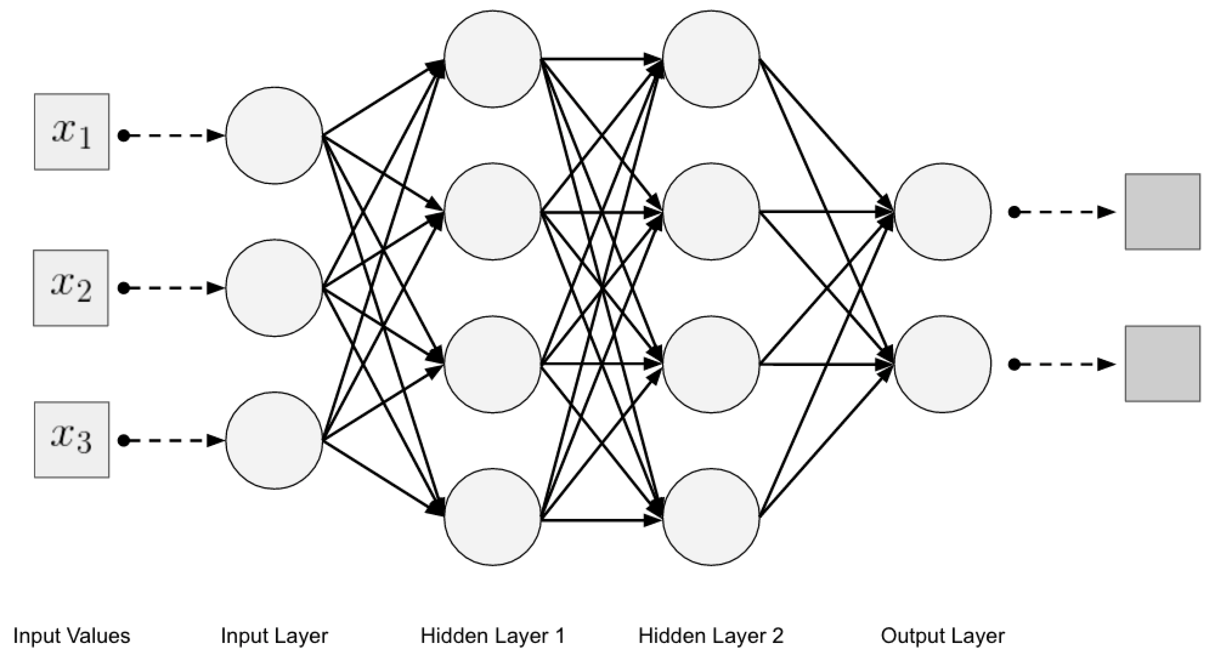
20]. The focus of this article will be on the pattern recognition of image data. The MLP architecture consists of at least three layers: one input layer, one or more hidden layers and one output layer. Each layer comprises several processing units or neurons. All neurons in one layer are fully connected to each neuron in the next layer, but they are not interconnected within a layer [
14,
16,
21]. The input layer only passes the raw data along. The output layer’s task is to convert the results from the hidden layers to an output, such as a classification category [
12].
Figure 2 shows an example of a multilayer neural network with two hidden layers.
One reason for its high success and popularity is that it is considered as a universal approximator, which means that it is capable of modeling almost any function when a sufficient number of hidden layers is added [
7,
19,
23].
2.2.3. Backpropagation: Learning a Function
Learning is an essential characteristic of all ANN algorithms [
24] and is usually achieved in two steps: forward propagation, followed by backward propagation [
18]. Backward propagation, or backpropagation, was introduced by Rumelhart, Hinton and Williams in 1986 and is fundamental for the learning behavior of neural networks [
24]. The forward propagation computes the output after processing the input data. The backpropagation starts at the output layer [
25], where it takes the computed output and compares it to the actual, desired output [
23]. It then adds up the squares of the differences between each component, called the squared error (SE). The formula considering one single input is defined as
where
SE represents the error rate,
d is the actual output and
f is the output that the network gives. To not just evaluate the performance of a single input vector, but the entire network, the loss function is used, which calculates the mean squared error (MSE) [
26] as follows:
where
represents the output of the function,
n stands for the number of data points in the training set and
and
represent the desired and actual output of the model for the data point
i [
27].
Backpropagation uses gradient descent to update the interconnection weights to minimalize the mean squared error in the network in many iterations [
24]. Typically, in the first training iteration, the interconnections of the network layers are assigned random weights. The resulting mean squared error is then broadcasted backward to the input layer to update the weights and therefore decrease the gradient.
2.2.4. Activation Functions
An activation function is applied to determine the output of the neurons, where each output of a neuron contributes to the final output of the network [
18]. The activation function models the firing rate of the artificial neuron, and usually, nonlinear functions are used to narrow the output (e.g., a threshold function limits it to 0 or 1; a sigmoid function between 0 and 1; and a hyperbolic tangent between −1 and 1) [
28]. Nowadays, it is strongly recommended to use the rectified linear unit (ReLu) in more modern neural networks. The ReLu function calculates the output using a ramp with
The ReLu function gives an output of
x if
x is positive and an output of zero if it is negative [
13]. As all negative outputs are set to zero, a fewer number of neurons will be considered in the propagation. This results in a more lightweight network that is capable of going through iterations quickly without significantly affecting the generalization accuracy [
3].
For multiclass classification problems, the softmax activation function is often used in the output layer. Softmax is a linear function that takes the activations from the previous layer to generate an output between 0 and 1 for each class. This output is interpreted as the class probability [
7].
2.2.5. Optimizers
Optimizers are used in the backpropagation process and help to minimize the error rate of the learning function. This is often achieved by using stochastic gradient descent (SGD). SGD leads to an optimization of the learnable parameters in the network, as well as to convergence to the local minima by performing parameter updates for each training example individually [
6]. There are a bunch of existing SGD options which all try to solve the problems of optimization. The most common optimizers are AdaGrad, RMSProp and Adam, although the publishers of the Adam algorithm insist that they combine both the benefits of the other two algorithms [
29].
2.2.6. The Problem of Overfitting
Another concern regarding backpropagation is that it only minimizes the error rate of the training data and not new data. This could have a negative impact on the generalization of the network [
5]. A model is said to be overfitted when it tends to remember features rather than learn them [
17]. This results in a much worse performance of new data and therefore loses its generalization, and it is not applicable to other datasets anymore [
18]. Overfitting depends on many variables, such as the size of the training data, number of training iterations, the bias and the number of layers and nodes. A large training dataset usually results in a better generalization of the model [
9,
26].
2.2.7. Conclusion: Neural Networks for Image Classification
Neural networks consist of a certain number of neurons, which try to mimic the biological neuron when processing inputs to generate a specific output. Backpropagation is used to improve the generated output by automatically updating the models’ internal structure to reduce the difference between the generated output and the correct output. For multiclass classification problems, ReLu is the standard to use for activation functions, while Adam is the most used optimizer.
2.3. Convolutional Neural Networks
A CNN is a deep artificial neural network that is widely known for its usage with image data. In some ways, its architecture is similar to typical neural networks, as it consists of fully connected layers comprising many neurons, which have learnable parameters such as weights and biases. The difference is that convolutional neural networks do not only consist of fully connected layers. They instead make use of convolutional layers combined with pooling layers, while fully connected layers are mostly used as the last layers of the network to generate an interpretable output. A big advantage of CNNs is that once a feature is learned by the network, it is recognized regardless of its position in an image. By stacking these three layers in different ways, a vast number of various architectures can be designed [
30].
2.3.1. Transfer Learning
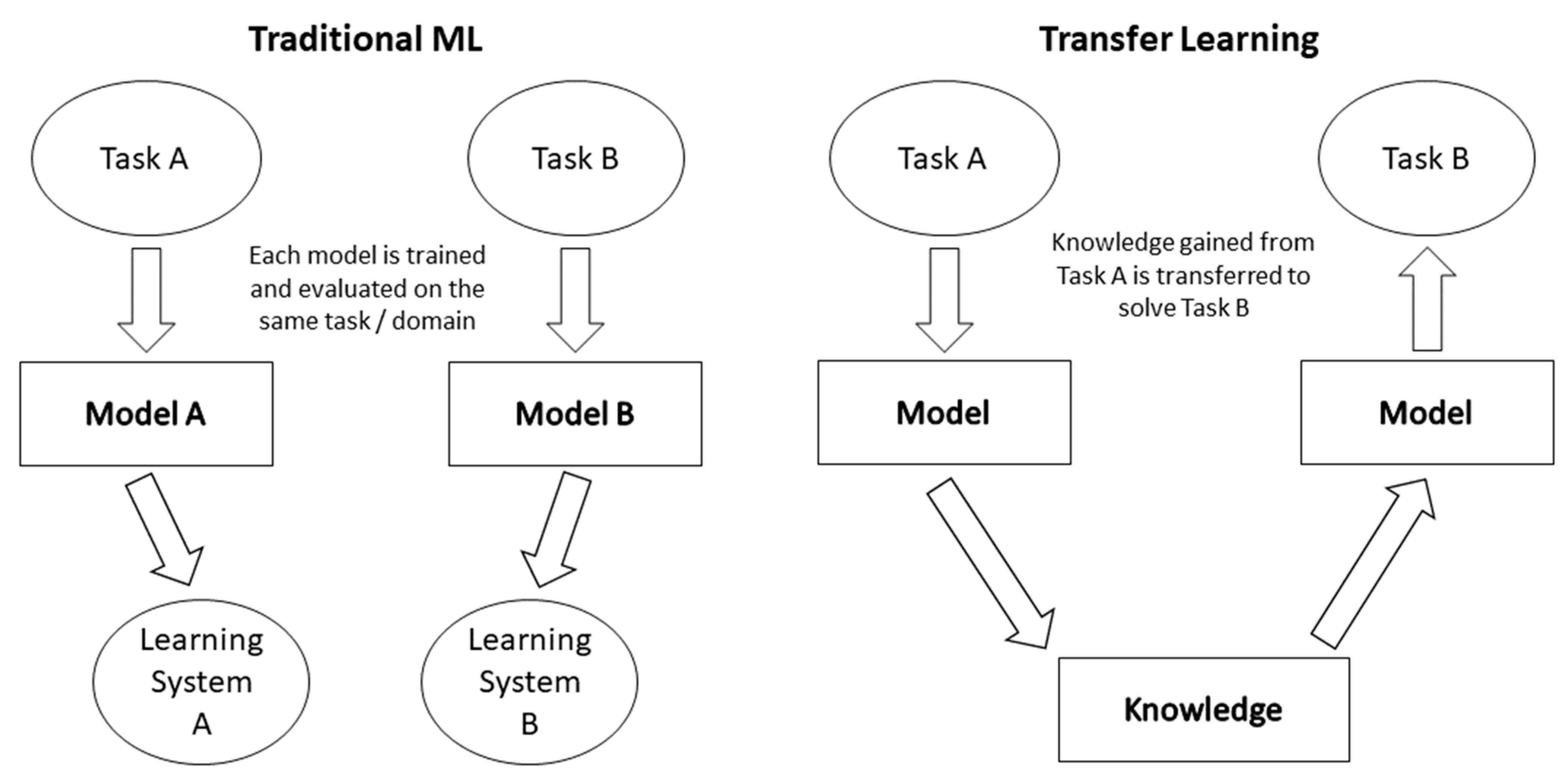
The idea of transfer learning is to understand new tasks easier through leveraging familiar conditions, and it is an approach closely related to learning by analogy. The main concern is the analogy between the source and the new target, which can even be in a completely different application. However, it is crucial that a sufficient analogy between the underlying datasets or tasks exists [
31].
Figure 3 shows the difference between traditional ML tasks and tasks that are accomplished using transferred knowledge.
Transfer learning can be used to train parts of a dataset separately and then transfer the results to the next part, which can be in a different algorithm [
32]. Transfer learning is a commonly used method in deep learning and can be especially useful in large-scale image classification applications, which require expensive computational power. In a CNN, it can also help to prevent overfitting when the training data set is too small. In these cases, a pretrained network is used instead of the usual random initialization.
2.3.2. Data Augmentation
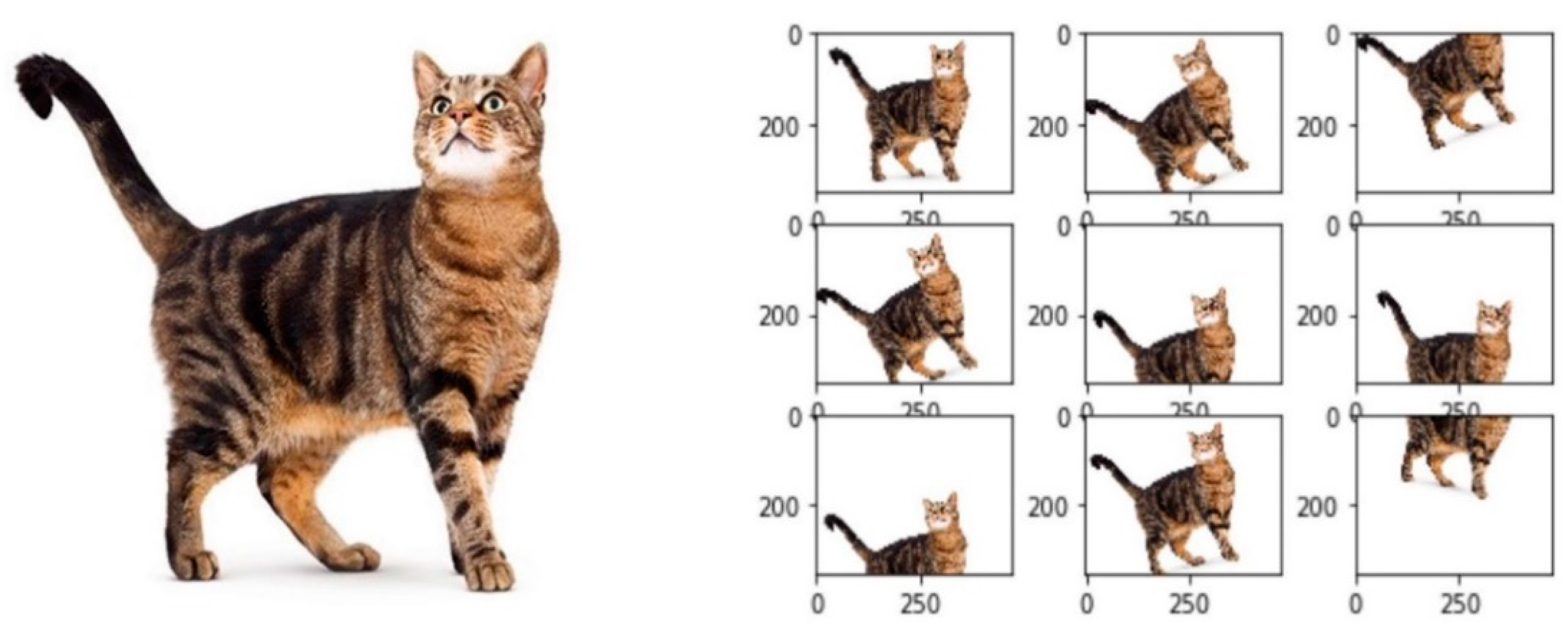
Data augmentation is a regularization method for deep neural networks. The best way to improve the performance of a neural network is to increase the size of the dataset. However, with image data, it often is difficult to acquire more data. One workaround is to create fake data from the existing dataset. This approach is especially appropriate for image classification tasks, as images are high dimensional and contain lot of variation factors. Therefore, it is important to compute image transformation without altering the corresponding class (rotating an image of the digit 6 by 180° would result in a 9).
With data augmentation, images can be, for example, rotated, flipped, scaled, translated or subsampled with various crops and scales.
Figure 4 shows how augmentation transforms images to amplify the dataset with fake data. In this example, the operation on one input image results in nine augmented fake images.
2.3.3. Important Layer Types
CNNs for classification purposes usually consist of three layers: convolutional, pooling and dense layers [
34]. To prevent overfitting, the dropout layer is indispensable as well.
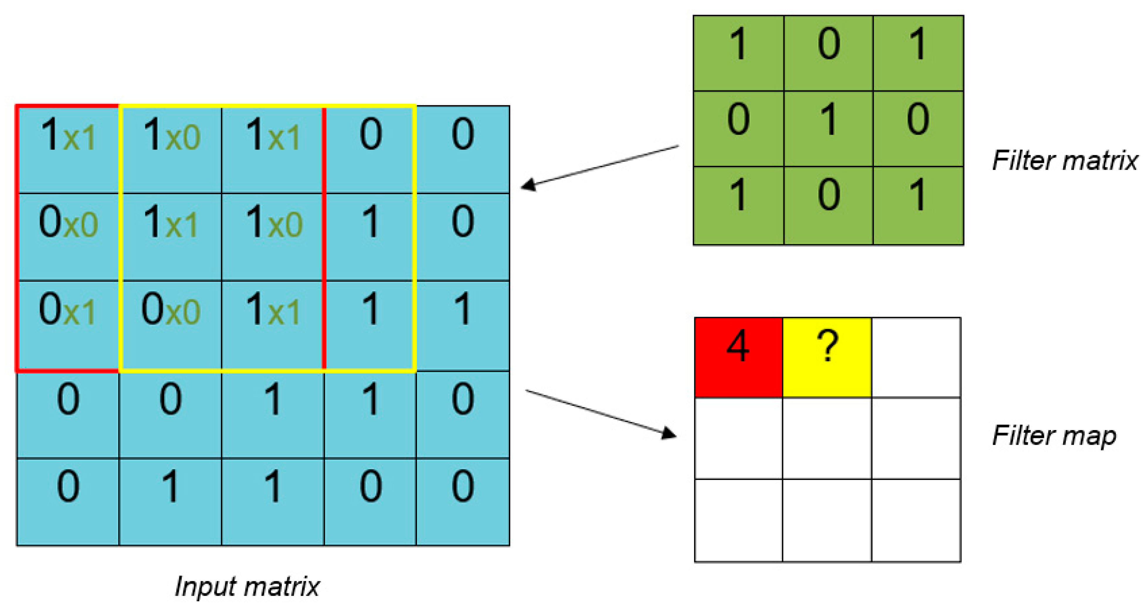
The convolutional layer is generally the first layer in a CNN after the input layer. At first, the input matrix is analyzed by a defined number of filters with a certain kernel size (e.g., 3 × 3). These filters then move from the top-left to the bottom-right with a defined step size, or stride. In addition to the stride and kernel size, a padding that decides what to do when the filter hits the edge of the matrix is defined.
Figure 5 demonstrates the calculation of the feature map for a two-dimensional input. The blue matrix depicts the input, whereas the green matrix depicts the filter. The filter matrix is multiplied with every distinct 3 × 3 subregion of the input matrix to form the feature map, starting from the top-left. The red marked square in the input matrix is called the receptive field. In the receptive field, the input values are multiplied with the filter values and summed up as
1 × 1 + 1 × 0 +1 × 1 + 0 × 0 + 1 × 1 +
1 × 0 + 0 × 1 +
0 × 0 +
1 × 1. This calculation results in four, the first value of the feature map. Here, the input values are on the left side with the multiplication, and the filter values are on the right side.
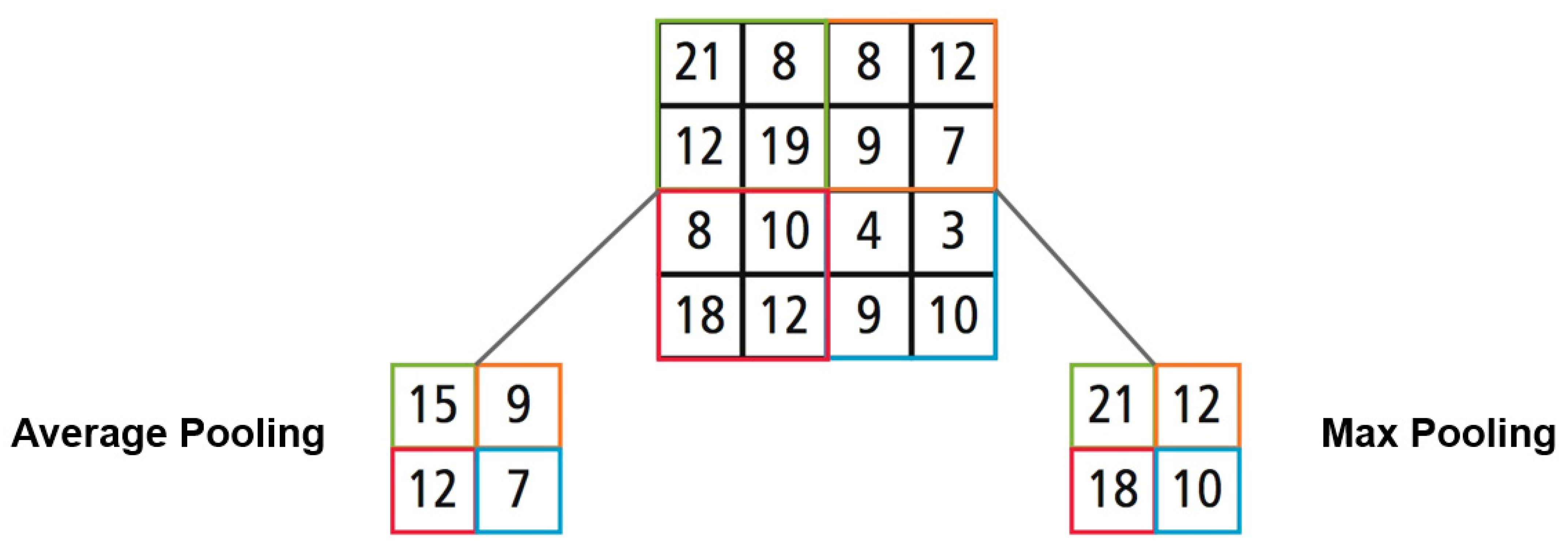
The second import layer type is the pooling layer and, in short, the main task of the pooling layer can be described as sampling down the previous input to decrease the complexity for the next layer. In image data processing, downsampling can be considered as reducing the resolution of the features in the image, which makes it resilient against noise. Two common ways have emerged to perform pooling: max pooling and average pooling. For both methods, a filter size and a stride are needed. The filter size describes how many values should be downsampled; usually, a size of 2 × 2 is chosen. The stride describes how many fields the filter moves and is usually chosen to be of the same length as the filter size. The pooling starts at the top-left of the input matrix and takes the first 2 × 2 subregion. As shown in
Figure 6 below, the two methods differ at this point; max pooling will just return the maximum of the four values, whereas average pooling will calculate and return the average value within the subregion [
12].
The dense layer is the only fully connected layer in a CNN with a linear connection from input to output, like how neurons interact in a traditional neural network. After the features are extracted by the convolutional layer and downsampled by the pooling layer, the dense layer’s goal is to perform classification. Therefore, it receives input from all neurons of the previous layer to process them in a linear input-to-output connection [
34]. In
Figure 7, the left model shows a densely connected neural network with two hidden layers.
Fully connected layers entail a vast number of parameters and can result in very expensive computations when used for high-dimensional image data. Because of this, it is mostly used only in the final or two final layers of the network [
12].
The use of dropout layers is an efficient way to prevent overfitting through model combination. A dropout layer sets the output of randomly chosen neurons to zero. Therefore, the dropped-out neurons neither participate in the forward nor in the backward propagation, meaning that the model builds a different architecture for every new input it receives. The percent of randomly dropped-out neurons is provided by the user. Due to this method, neurons tend to rely less on the presence of other neurons and decreases the possible complex coadaptions of neurons [
35].
2.3.4. Conclusion: Convolutional Neural Networks
CNNs depict input images as matrixes of numbers, which represent the pixel values of the image. Typically, CNNs consist of three different layers—convolutional layers, pooling layers and fully connected layers—where the convolutional layers build the core part of a CNN. CNNs learn the features in images regardless of their position in the image. When it comes to multiclass image classification problems, convolutional neural networks are the standard and will also be used to implement the image classifier for fashion images in this article.
In real-word applications, it is often a difficult task to collect a big dataset that is necessary for a successful neural network. With the help of data augmentation, more data can be created by rotating, scaling, cropping, flipping or zooming the original input images. Through these operations, the dataset is enlarged with fake data and can lead to an improved generalization of the network.
Transfer learning is a machine learning approach that is mainly used when dealing with small datasets. Its focus is to store the knowledge from one application scenario to later use it on a different but related application scenario to save computational resources and make use of a bigger but different dataset. Transfer learning can lead to an improved generalization of the network and a decreased training time. In addition, several options for well-established CNN architectures were presented to perform transfer learning on.
3. Set-Up for Case Study
For the practical part of this paper, the main task was to implement a CNN to see how well a classifier performs on a small fashion dataset. To properly test the performance, four approaches are used. First, a model is trained on general data (i.e., the fashion MNIST dataset) to test how it performs on new, specific tasks. Secondly, a model is pretrained on the fashion MNIST dataset and fine-tuned with a created training dataset. The last approach trains the model only with the created training dataset, without using the fashion MNIST dataset.
3.1. Hardware
One of the major limitations for the usage of deep learning methods is the need for computational power and the high amount of training data that is needed to produce generalizations. For the training phase of the CNN in this article, neither a server farm nor a top-notch Graphics Processing Unit (GPU) was available. Therefore, the neural network was trained on a running Proxmox 6.0-4 virtual environment on a Linux server with following technical specifications:
Linux/Ubuntu server as a virtual machine;
DELL Poweredge R730;
Processor: Two Intel(R) Xeon(R) CPU E5-2640 v4 @ 2.40 GHz;
Drive: 256 GB SSD;
RAM: Ten DDR4-2666 with 16 GB.
Training a deep neural network from scratch without using a proper GPU is tremendously time-consuming. Thus, the transfer learning method is applied to make use of an already successfully established CNN to try to save computational power. The training time will not be evaluated precisely, but it will be tracked and analyzed to see if techniques like dropout, data augmentation or transfer learning have an impact on the training time.
3.2. Libraries and Frameworks
The best-suited framework for a network depends on the network itself and on the preferences of the people who are building it.
Table 1 depicts the ranking of the most popular open software libraries based on stars and forks, which are received from the GitHub community [
36].
In this article, TensorFlow will be used as the backend, and Keras will operate on top of it. Both will run in an Anaconda environment using Jupyter Notebook. The following subsections will explain the chosen frameworks and justify the selection.
3.2.1. TensorFlow
TensorFlow is open-source, rapidly evolving and backed by a strong industrial company. Therefore, it is widely considered as the most popular and most used deep learning tool. The high popularity can also be seen in
Table 1 [
37]. The main advantages of TensorFlow are as follows:
It already offers multilanguage support, with a foreseeable increase in supported languages in the future;
Its high performance;
Its support for multi-Central Processing Units (CPU), GPU and even hybrid platforms;
Its high portability.
Because of the already-established popularity and the support received from Google, it is foreseeable that TensorFlow will have major advantages to the deep learning frameworks that are maintained by individuals or universities in the future [
38].
3.2.2. Keras
Keras is another deep learning library written in Python, and it makes use of either Theano or TensorFlow as its backend. Keras is built on four principles [
37]:
Keras was designed for humans, not machines, and therefore offers Application Programming Interfaces (API) that are consistent and simple to use.
- 2.
Modularity;
Neural layers, optimizers, activation functions, cost functions, initialization schemes and regularization schemes all act as independent, fully configurable modules and result in the model when they are plugged together.
- 3.
Easy extensibility;
New required modules are easy to add, and already existing modules are provided with sufficient examples to reach clarification.
- 4.
Work with Python.
The use of Python makes the models easier to debug, more compact and enables easy extensibility.
3.2.3. Anaconda
Anaconda is an open-source distribution for performing machine learning and data science tasks in Python and R, either on Windows, Linux or Mac OS X.
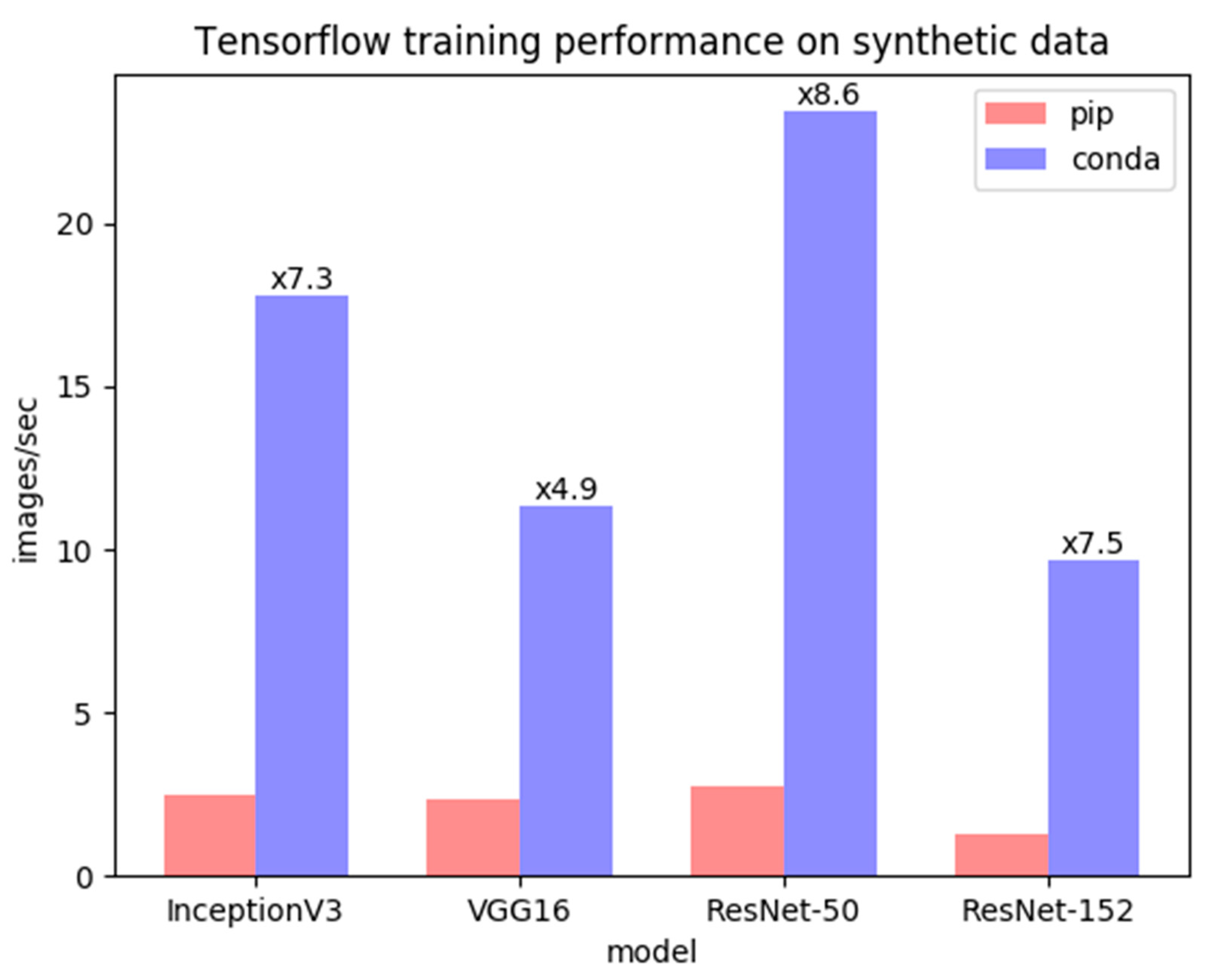
Figure 8 compares the training and inference performances of four different image classification models, where TensorFlow is installed once with conda and once with pip; both used the same version. As can be seen, the performances of the models installed with conda were significantly better in speed than the performances of the models with pip in all of the four cases [
39].
Anaconda is the leading integrated development environment (IDE) for data science projects and particularly offers great performance and integration with TensorFlow. Keras, TensorFlow and Anaconda harmonize excellently with each other and build the foundation of many CNN projects.
3.3. Datasets
This section describes the fashion MNIST dataset, which is the standard for benchmarking computer vision and deep learning models. However, this section also describes the creation process of the training and test datasets, which will be classified in the course of this article.
3.3.1. Fashion MNIST Benchmark
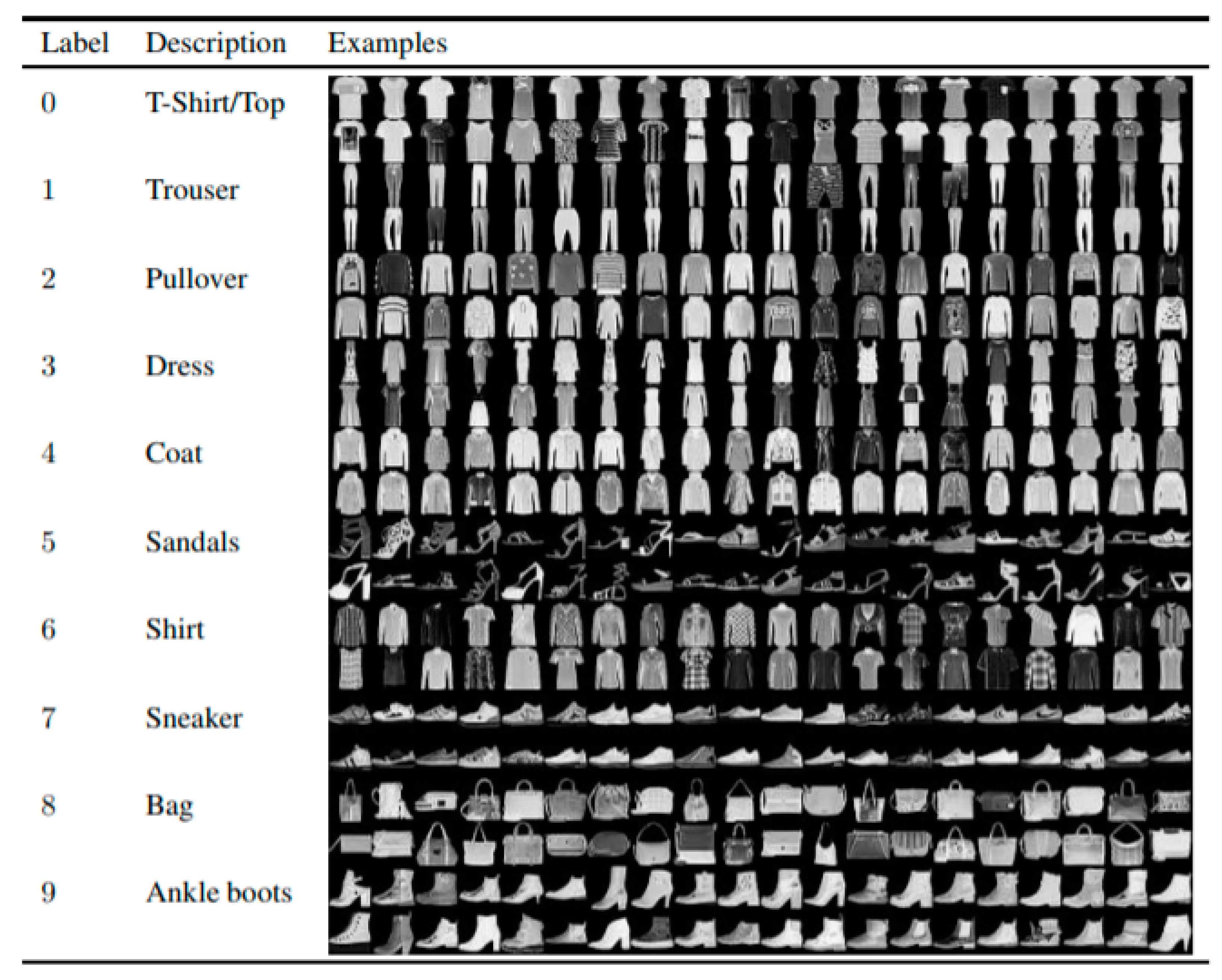
The original MNIST dataset consists of handwritten digits and was used as a benchmark for machine learning algorithms over the past few years. The fashion MNIST dataset consists of 70,000 article images provided by Zalando. The dataset is split into a training set containing 60,000 images and a test set with 10,000 images. Each data entry is a grayscale image of the size 28 × 28 and belongs to one of the 10 class labels shown in
Figure 9.
3.3.2. Created myFashion Dataset
The to-be-implemented network model used supervised learning, and thus it needed labeled data for the training phase. The image data was gathered and downloaded with the Fatkun Batch Download Image extension for Google Chrome. The Fatkun extension downloads all selected images for a specific Google query. The following table shows the key search phrases that were used for the data collection process.
The created dataset consisted of 2567 images, which were divided into 10 classes. As can be seen in
Table 2, the classes within the dataset had a balanced image count. With 288 images, dress was the class with the highest image count. The hat class, on the other hand, comprised the fewest images with just 202. Besides these two classes, the margin between the other eight classes was relatively small and reached from 232 to 281 images. The dataset consisted of human-worn fashion images. The images could be both indoor and outdoor, and all had different backgrounds. Before preprocessing, the dataset had a size of 191 MB. All images were color images and were of different dimensions. The created dataset will from now on be referenced as the myFashion dataset.
The myFashion dataset was split into training and testing datasets with a proportion of 80:20. The training dataset will be used for network training, while the testing dataset will be used to evaluate the model.
3.3.3. Potential Difficulties with the Dataset
- 1.
Size of the dataset;
With just roughly 2600 images, the size of the dataset is rather small and usually not sufficient to reach a generalizable result with the model. Because of this, data augmentation will be used to significantly enlarge the dataset.
- 2.
Images can contain more than one fashion class.
Another potential problem is that the model will classify each input image into one certain class. However, it is possible that some of the images contain more than one class feature, such as a person wearing a bag and trousers. In this case, the network is much more error-prone and could end up making wrong classifications easier than normal.
4. Implementation
4.1. Approach
To see if the models’ performances—measured in accuracy and loss rate—could be incrementally improved, the following four approaches were defined:
- 1.
Classifying fashion MNIST;
To find the most accurate architecture with the highest accuracy, several models would be trained. These to-be-implemented models were based on the AlexNet architecture and, to figure out the most suitable architecture, they would differ in following characteristics:
To ensure the same training conditions, as well as to decrease the number of models, the following training parameters would be the same for all models:
Optimizer = Adam;
Activation function = relu and softmax;
Kernel size = 3 × 3 pixel;
Max pooling = 2 × 2 pixel;
Batch size = 64;
Training epochs = 50.
To show if the dropout layers could help prevent against overfitting, each model was trained one time with dropout layers and one time without. If dropout layers were added, they would be applied after each convolutional layer and the first fully connected layer with a value of 0.4. The model architecture that achieved the best validation accuracy would be described and presented in the next section. In addition, the weights of the most accurate model would be saved and used for transfer learning in the third approach.
- 2.
Classifying the myFashion Dataset;
The model with the best performance in the first approach would be used for this approach as well, but in this approach, the collected images of the myFashion dataset would be classified. Here, the network would be trained one time with data augmentation and one time without data augmentation. This should show if data augmentation could further improve the performance of a model trained on a small image dataset. Furthermore, if applying data augmentation turned out to be helpful and improved performance, it would also be used for the third and fourth approach.
- 3.
Transfer Learning with MNIST;
In this approach, the model would be initialized with the saved weights from the most accurate model of approach one, meaning that the same architecture must be used, including the input layer with the same input shape. This could negatively affect performance, as the myFashion dataset mainly consists of large color images. Furthermore, to see how well the myFashion dataset could be classified based just on the knowledge gained from the Fashion MNIST, all convolutional layers would be frozen. This means that the weights within the layers would not be updated during the training phase. Therefore, every single time an input image was put into the frozen pretrained network, it would result in the same class. The theory says that transfer learning can be used to save computational resources and, as a result, also save time. To prove the theory, the training time would be measured for this model.
- 4.
Transfer Learning on ImageNet with VGG-16 and GoogLeNet.
With the help of Keras’ application module, already-established deep learning models could be easily imported alongside their pretrained weights and be used for feature extraction. However, as the model should now fulfil a different classification task, it was essential to import the model without its last layers and add our own fully connected layers that were necessary to classify the myFashion dataset. For this purpose, four fully connected layers would be added, whereas the first two fully connected layers were followed by dropout layers. Furthermore, to efficiently make use of the transferred knowledge, all weights in the convolutional layers would be frozen so that they would not be updated during the training phase. As ResNet requires the most computational power and hardware capabilities, VGG-16 and GoogLeNet were the most suited and would be used for this approach.
Preprocessing
As the created myFashion dataset was too small to perform a generalizable image classification, data augmentation was used as described in
Section 2.3.2. The Keras module ImageDataGenerator did all the work for labeling, preprocessing and loading the dataset. To decrease the computational power required, all images were divided by 255 to receive values between 0 and 1. Furthermore, the dataset would be significantly increased by performing the following image operations:
Rotating the image by a specific degree value;
Moving the image vertically and horizontally by a relative value between 0 and 1;
Zooming randomly inside the image by a float value;
Flipping or mirroring the image on the horizontal axis by setting the value to true or false;
Filling the pixels that were newly created (e.g., by image rotation or zooming).
The following argument–value pairs were passed to the ImageDataGenerator:
After successfully specifying the ImageDataGenerator, the datasets were loaded to the network with the flow_from_directory function. Given a directory, it loaded all subdirectories to the network and assigned the label of their parent folder to the images. This function again took some beneficial arguments to ease the set-up for the training phase. For this purpose, we wanted to set the following parameters:
Directory path to load the datasets;
Required target size of the images in the shape of (height, width);
Required color mode of the loaded images can be either set to grayscale or color images defined by the primary colors: Red, Green, Blue (RGB);
Class mode to determine the return type, either binary, sparse, categorical, input or none;
Batch size that was fed into each training iteration.
The following argument–value pairs were passed to the flow_from_directory function:
In conclusion, the images were cropped from different dimensions to color images 64 × 64 pixels in size and feed to the network in batch sizes of 32. As the class mode was set to categorical, the network returned exactly one predicted class for each image.
5. Evaluation and Results
In this section, the four described approaches to build an image classifier for feature extraction in fashion data are evaluated by their validation accuracy, and the results of the experiments are presented. It should be noted that the models from approach two, three and four are all evaluated on the same test dataset. For these evaluations, the confusion matrix will be calculated to compare the implemented models by their respective f1-scores. The validation accuracies were calculated with the built-in evaluation module of Keras.
Table 3 displays the best-performing models that were trained on fashion MNIST to find the most appropriate model to work on fashion data. As the input shape of the images was 28 × 28 pixels and each max pooling layer was cutting the image in half, a maximum of four convolutional layers could be used. All models were compiled with the following parameters:
Finally, the model was trained with following settings:
Train_generator = train_generator.flow_from_directory([path_to_parent_directory]);
Steps_per_epoch = train_dataset_size/batch_size;
Epochs = 50;
Validation data = test_generator.flow_from_directory([path_to_parent_directory]);
Validation steps = test_dataset_size/batch_size.
The architecture column in the table defines the layers that were used to build the model. The values in the brackets describe the number of filters or units within the layer. Model number 1.4 will be described to clarify the format. The model comprised three convolutional layers. The first one, the so-called input layer, comprised 32 filters, the second 64 and the third one 128. For classification, two dense layers were used. The first one consisted of 128 neurons, and the last layer consisted of 10 neurons, where each neuron represented one of the 10 fashion categories. In this table, the validation accuracy column displays the evaluated accuracy of the model for training under the following conditions:
Without dropout layers;
With dropout layers.
As can be seen from the table, the performances of the different models did not differ too much in their validation accuracy. Basically, models with four or more convolutional layers resulted in rather worse performance compared with models with three or fewer convolutional layers. Furthermore, all models that were trained with three convolutional layers reached a validation accuracy above 93%. Based on the performed model evaluations in
Table 3, we can conclude that models with three convolutional layers were best suited for classifying fashion images. On the other hand, the number of fully connected layers and its respective units did not significantly affect the validation accuracy.
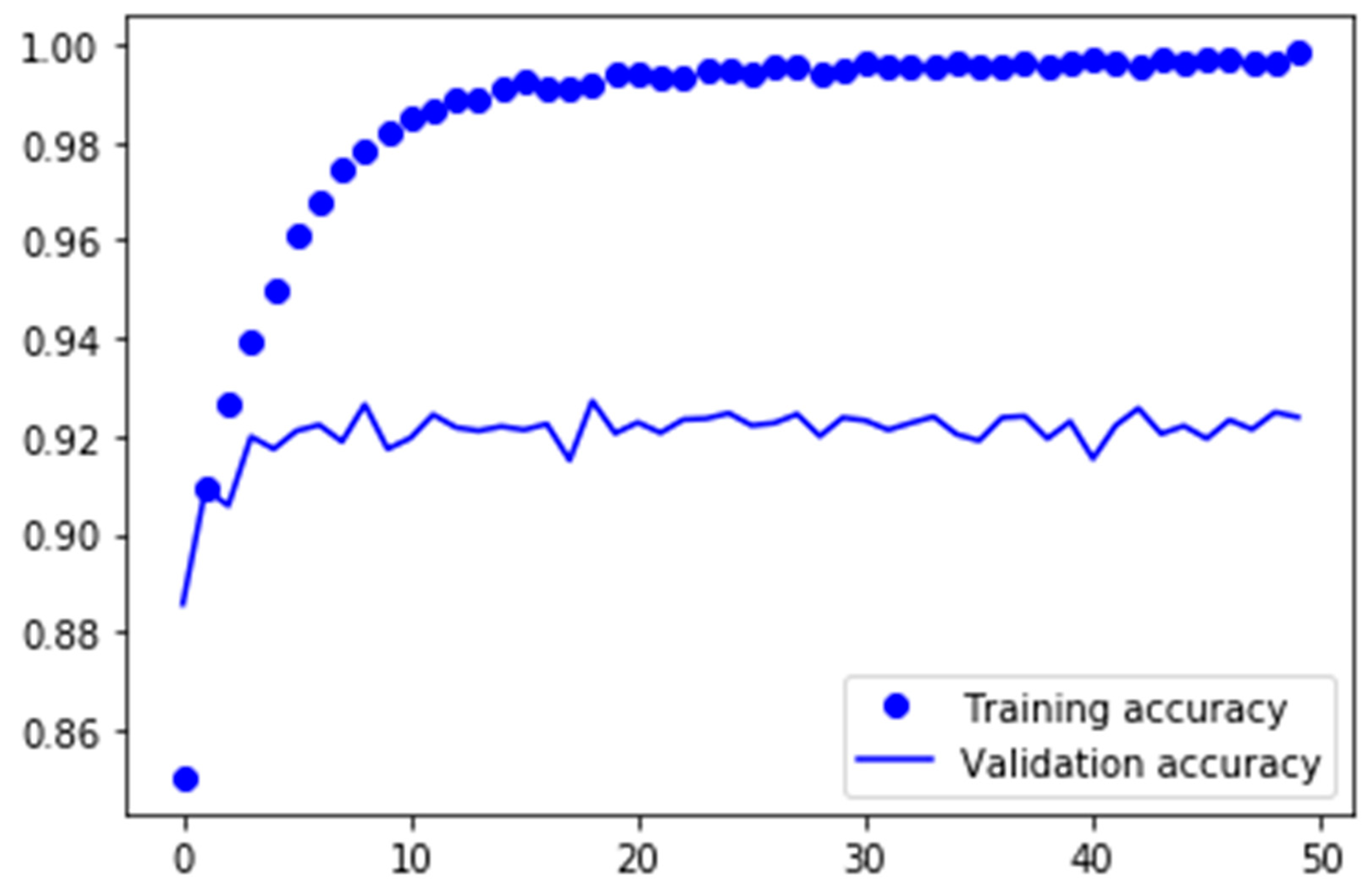
Next, we can see that all models that were trained with dropout layers achieved a higher accuracy than the ones that were trained without them, even if the differences were minimal at some models. Model number 1.11, the model with the highest validation accuracy, reached a training accuracy of 99.27% and therefore classified almost every single training image correctly when it was trained without dropout layers. However, when it had to process new, unknown data, the accuracy dropped by more than 7% to a final 92.02% validation accuracy. This can be interpreted as a result of overfitting, as the network tended to capture and memorize the image features instead of learning them.
Figure 10 plots the training and validation accuracy over 50 epochs without dropout layers.
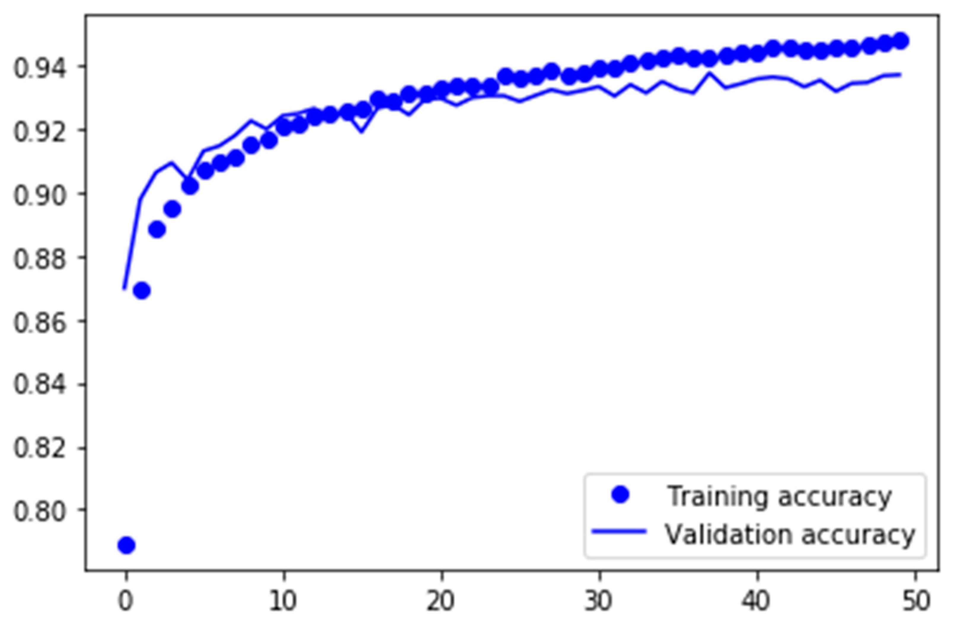
In
Figure 11, the same model trained with dropout layers is plotted, and the difference is quite clear to see. The gap between the training and validation accuracy almost vanished when dropout was applied.
This implies that we can assume that dropout regularization helps to prevent against overfitting, and at the same time, it can improve the models’ generalization abilities for new data the network has not seen before. As was already stated before, deeper models usually take longer to train, and to put that into perspective, models 1.4, 1.9, 1.10 and 1.12 were adduced and compared in
Table 4. Models 1.9 and 1.10 had the same number of layers and just differed in their number of neurons and filters within these layers. Model 1.9 came to a total of 495,434 trainable parameters, while model 1.10 consisted of more than 1.6 million, almost four times more parameters. Model 1.4 featured one additional convolutional and max pooling layer compared with model 1.12, but this one extra convolutional considerably reduced the number of parameters fed into the fully connected layers and, subsequently, the number of parameters of the model as well.
In conclusion, it is important to find the right number of convolutional layers that is needed to successfully extract features while maintaining solid performance by reducing the total parameters of the model. It is worth mentioning that applying or not applying dropout layers did not significantly affect the training time.
5.1. Winning Model Architecture
This subsection describes the model that is going to be used for classifying the myFashion dataset alongside its components and parameters. It is based on the winning model that achieved the highest accuracy for the fashion MNIST dataset in the previous subsection but uses a different input shape.
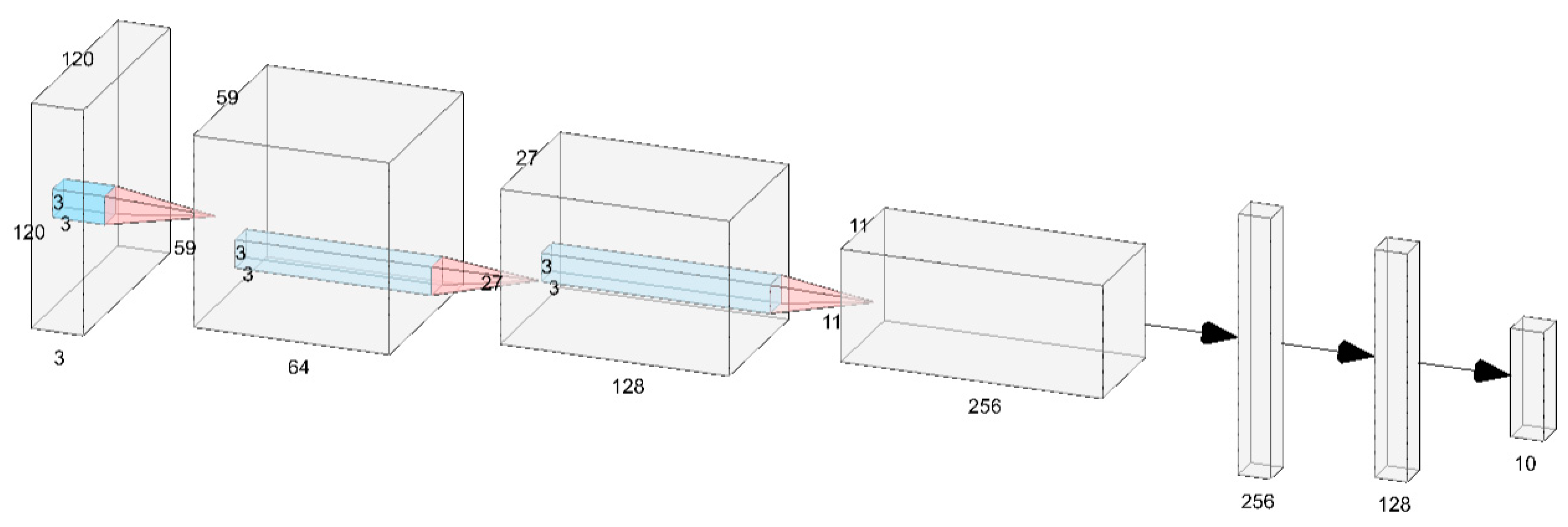
The architecture of the used model is demonstrated in
Figure 12. Altogether, the neural network contained six layers. The first three were convolutional layers, and the remaining three were fully connected layers. For the first convolutional layer, a stride of 2 × 2 pixels was defined, and the remaining convolutional layers had a stride of 1 × 1 pixel. Just by increasing the stride in the input layer to 2 × 2 pixels, the number of total parameters was reduced from 11.5 million to only 2 million trainable parameters. The last fully connected layer fed its output to a 10 way softmax activation layer, which mapped the final output to a distribution over the 10 class labels.
In 2012, Krizhevsky et al. showed that deep convolutional neural networks that used rectified linear units (ReLU) as activation functions trained many times faster than equivalent neural networks that used tanh activation functions. Since then, ReLU has been considered the standard activation function, and it was also used for all but the last layer in this model. For the last fully connected layer, the softmax activation function would be used to distribute the probabilities over the 10 classes.
Due to limitations in technical resources, the training was done on a CPU in place of a more-suitable GPU. This will potentially lead to an enormously increased training time but will not affect the accuracy of the model.
To reduce overfitting and improve the generalization of the model, dropout was used. Three dropout layers were added to the network: two after the convolutional layers, and the last dropout layer was added after the first fully connected layer. A dropout value of 40% was used.
As already defined beforehand, max pooling with a filter size of 2 × 2 pixels was used instead of average pooling, as it used simpler computations that would save some computational resources. The kernel or filter size of the model was set to 3 × 3 pixels with a different number of filters in each convolutional layer, and the Adam optimizer was used to minimize the error rate.
The following performance evaluations in the next two sections were performed using the 10 class model architecture described in this section.
5.2. Classifying the myFashion Dataset
This performance evaluation was performed using the 10 class model architecture of the previous section. With roughly 2600 images, the dataset was rather small, and in order to achieve higher accuracy by maximizing the use of the data, the myFashion dataset was split into 90% training data and 10% test data. The input shape of the images that were fed to the network was 120 × 120 pixels. The first model in the table was trained without both dropout and data augmentation. In model 2.2, the input data was loaded without preprocessing, and in model 2.3, data augmentation was used for preprocessing as described in
Section 4.1. For evaluation of the different models in
Table 5, the confusion matrix was used to calculate the F1-score. The F1-score would then be used to compare the models with each other.
As can be seen in
Table 5, the two approaches gave the following results:
Without both dropout and data augmentation, the model achieved a validation accuracy of 69.74% and an F1-score of 0.64. The model was trained for 79 min;
Without data augmentation, the neural network achieved a validation accuracy of 71.04%, and it took the network 35 min to train over 50 epochs. This resulted in a rather low F1-score of 0.68;
With the use of data augmentation, the network achieved a validation accuracy of 79.16%. The network was trained over 50 epochs, and training took 42 min. The model resulted in a final F1-score of 0.78;
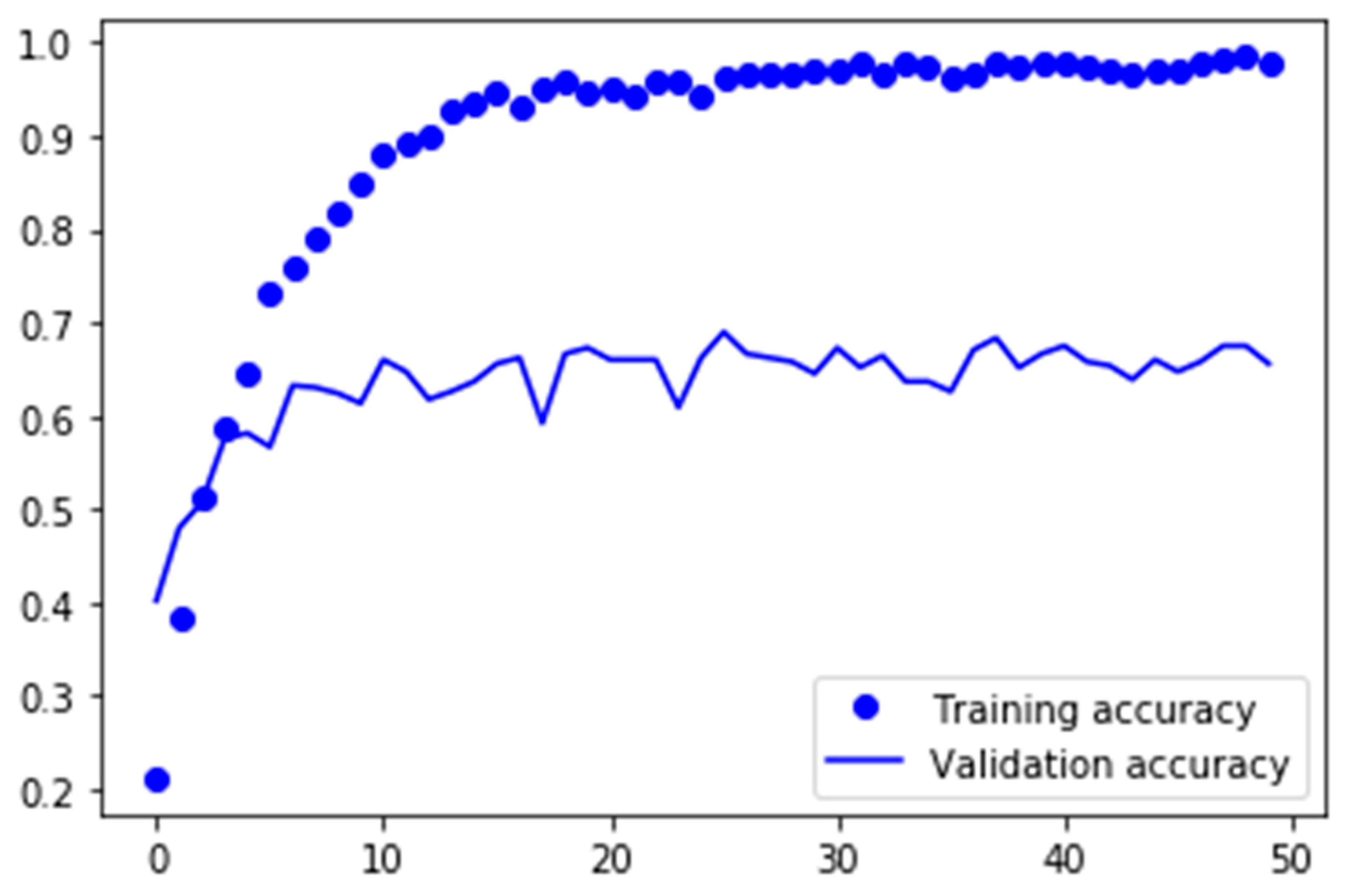
Figure 13 plots the training and validation accuracy of the first approach. Looking at the big gap between the training and validation accuracies in the plot, it is clear to see that the model was overfitted. Overfitting is a common problem when dealing with rather small datasets and makes the model not applicable for new and unseen data. In this model, the use of dropout was not enough to successfully prevent the model from overfitting. In the next step, data augmentation was used for preprocessing the data and to enlarge the training dataset.
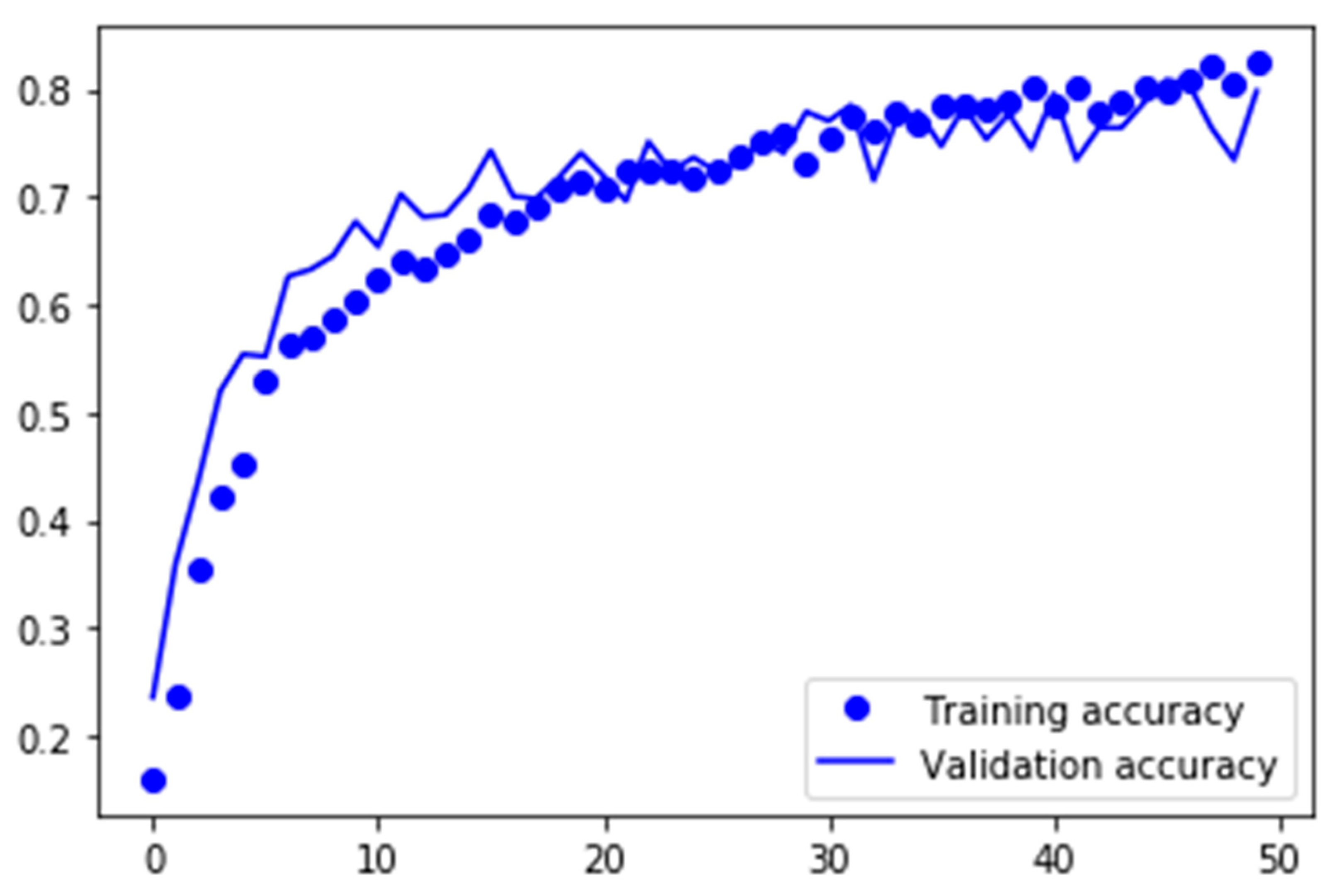
Figure 14 plots the training and validation accuracy of exactly the same model, with the only difference being that the input data was preprocessed with data augmentation. By just enlarging the dataset with fake data, the problem of overfitting vanished, and at the same time, the validation accuracy improved from 71.04% to 79.16%.
Due to the data augmentations, images were horizontally flipped, rotated, zoomed in and out and randomly shifted so that the features were not always placed in the center of the image. The image data augmentations meant that the neural network had to learn more robust, complex features and could not memorize the images as simply as with the myFashion dataset solely.
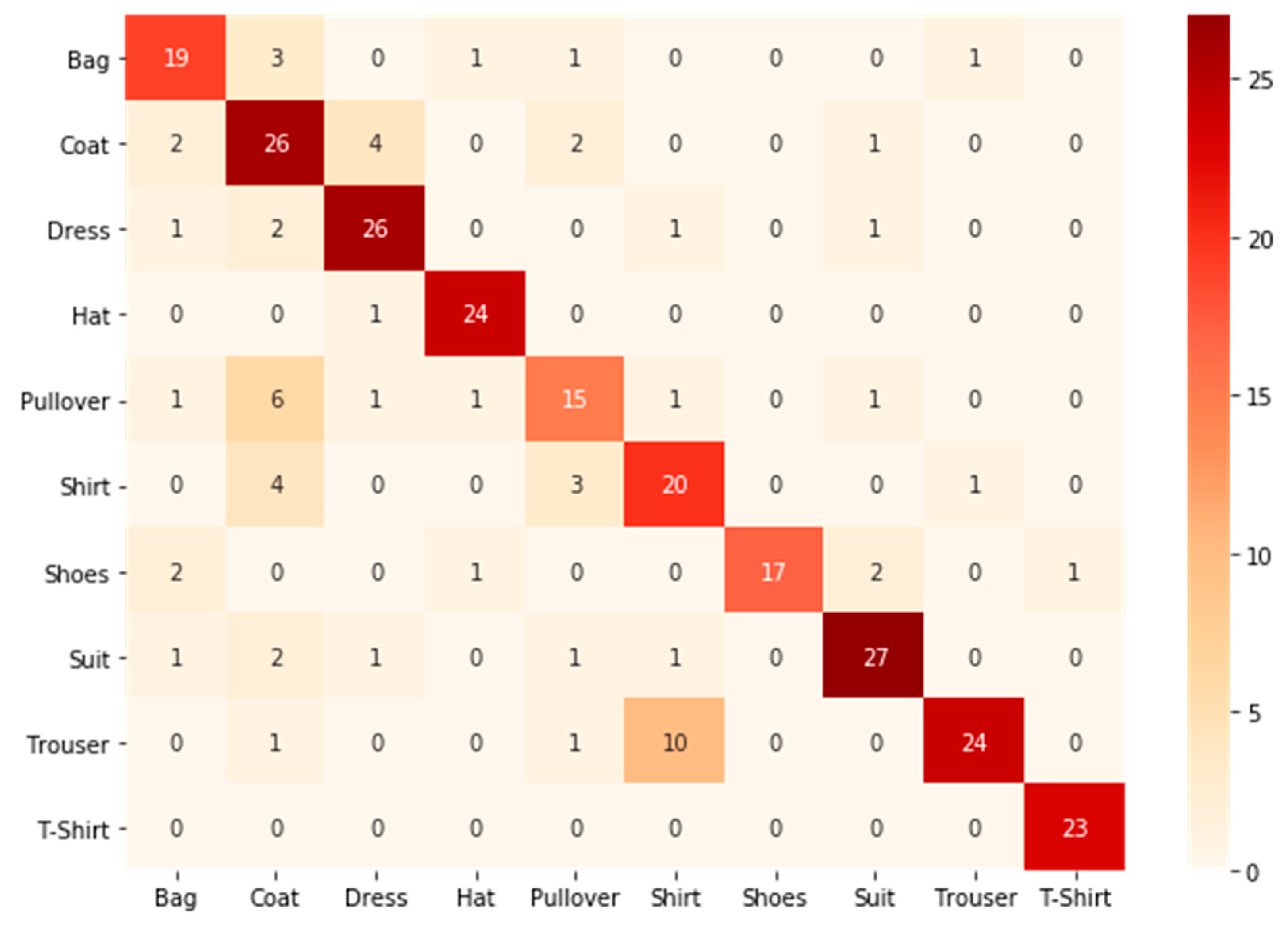
To further analyze the models’ performances, the confusion matrix was calculated with the test dataset, and it is presented with the classification report below. In
Figure 15, the confusion matrix is given. The red diagonal from the top left to the bottom right describes all correctly classified images for each class. The precision column in the classification report in
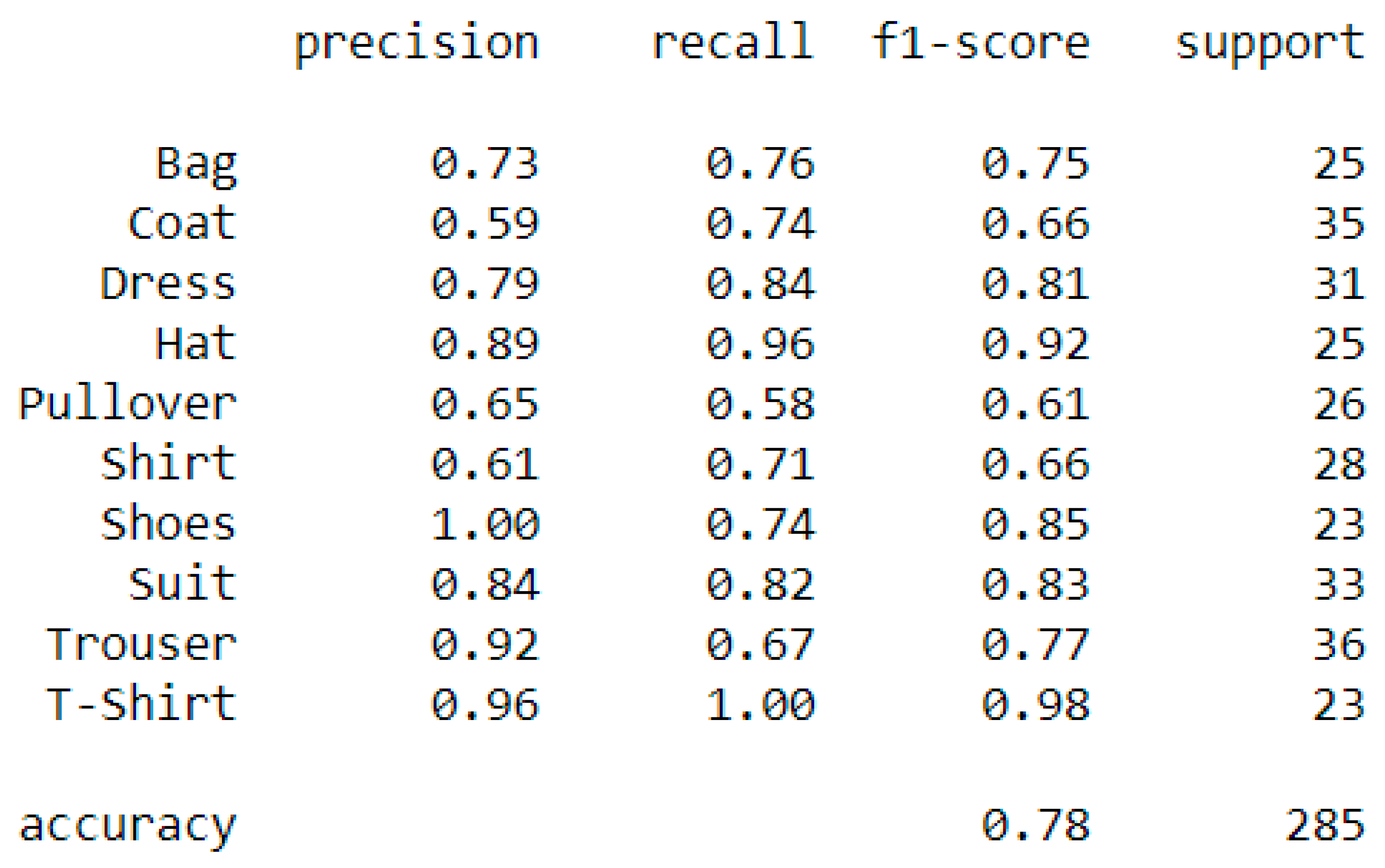
Figure 16 indicates how many images of all the test data were classified as class X and how many actually were in class X. For example, in the seventh column, there is one cell with 17 entries, and all other cells in this column are zero. This means that out of all the test data points, the classifier predicted 17 images as shoes, and all of them were shoes. This resulted in a precision of 1, or 100%. Recall, on the other hand, indicates how many of the test data of a certain class were predicted correctly. For example, in the first row, there is a total of 25 test images for the bag class. Out of these 25 images, 19 were predicted correctly, resulting in a class recall of 0.76. The F1-score describes a weighted mean between recall and precision and is, in general, lower than the accuracy and should not be interpreted as accuracy. However, it can be used to compare classes or even classification models. The support is the total number of appearances of the respective class in the dataset.
In
Figure 16, the classification report is shown. Looking at the F1-score, pullovers were classified the worst and t-shirts the best. The remaining eight classes reached F1-scores between 0.66 and 0.92. Hence, there was big classification fluctuation between the classes. The report also showed that all t-shirts were correctly predicted. In addition, 10 out of 36 trousers test images were wrongly classified as shirts. This indicates that the model had problems with distinguishing between trousers and shirts, and this could be a result of when some images entailed both classes. The model achieved an overall F1-score of 0.78, and this score would be used for comparison with other models.
5.3. Transfer Learning with the Fashion MNIST Dataset
In this section, the third approach will be evaluated. For this evaluation, the best model of approach was saved and loaded with its weights for transfer learning. In the previous model evaluation, we proved the importance of data augmentation when dealing with smaller datasets. Therefore, for the upcoming models, data augmentation would be used for the preprocessing phase. Furthermore, as the input shape of the fashion MNIST images was 28 × 28 pixels, and the color mode was grayscale, the same settings were used for this model. In
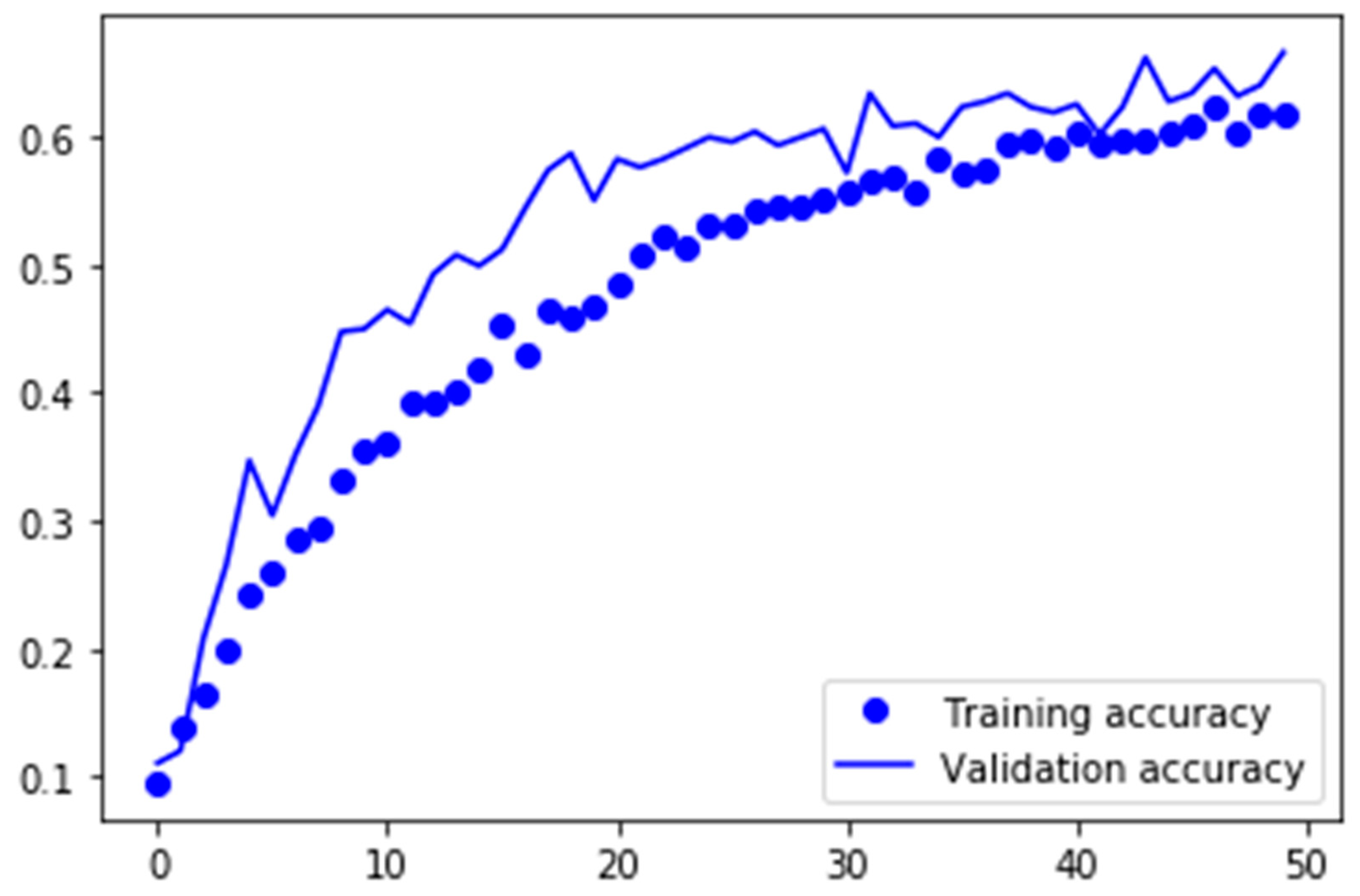
Figure 17, the training and validation accuracies of the model are plotted over 50 epochs.
In this plot, the validation accuracy is higher than the training accuracy. This could also be a result of when dropout was applied. Because 40% of all neurons were dropped, the data never passed through the whole network in the training phase. However, when the model was validated, the whole network was used, and this could lead to further improvement of the validation accuracy. The training time, validation accuracy and the f1-score were summarized in
Table 6 and shows that the training phase only took 12 min, which was approximately 30 min less compared with the models that were trained without transfer learning. Alongside the training time, the validation accuracy decreased by 16% to a validation accuracy of 63.12%. To conclude, transfer learning saved computational resources and could significantly reduce the training time of a neural network. However, the fashion MNIST dataset was not suited for transfer learning to classify human-worn fashion images. This assumption was also reflected by the low F1-score of just 0.38.
5.4. Transfer Learning with the ImageNet Dataset
The two deep learning models, VGG-16 and GoogLeNet, were both trained on the ImageNet dataset, but consisted of different architectures. This section is going to show which of these two deep learning models was most suited for classifying human-worn fashion images and if the validation accuracy of 79.16%, which was reached in
Section 5.2, could be further improved with transfer learning.
Table 7 gives an overview of the evaluated models with their respective training times and validation accuracies. With just 59 min, GoogLeNet was the fastest to finish the network training. In contrast, VGG-16 needed 1 h and 47 min.
Furthermore, VGG-16 was able to improve the validation accuracy reached in
Section 5.2, where the myFashion dataset was classified without transfer learning. VGG-16 achieved a validation accuracy of 83.96% and hence improved the performance by more than 4%. GoogLeNet, on the other hand, achieved a validation accuracy of 76.63%, which was a decrease of about 3%.
The evaluation plot in
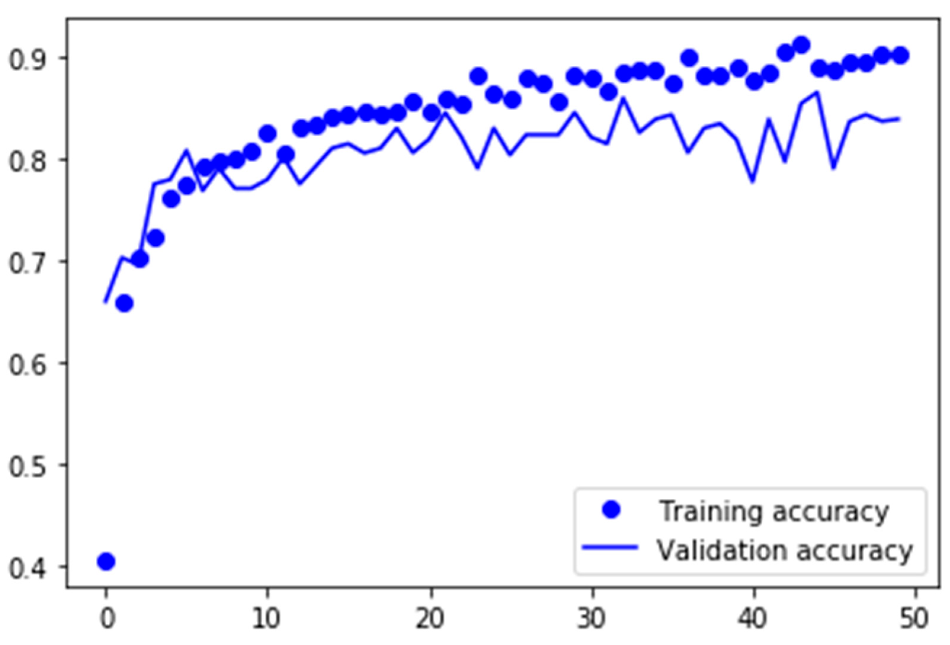
Figure 18 shows that transferring the knowledge from VGG-16 worked quite well. The model started with a validation accuracy of more than 65% in the first epoch of the training, which was significantly better than the validation accuracies of the previous models in their first epochs. It can also be seen that the validation accuracy was rather consistent over the 50 training epochs, with small fluctuations between 78% and 84%.
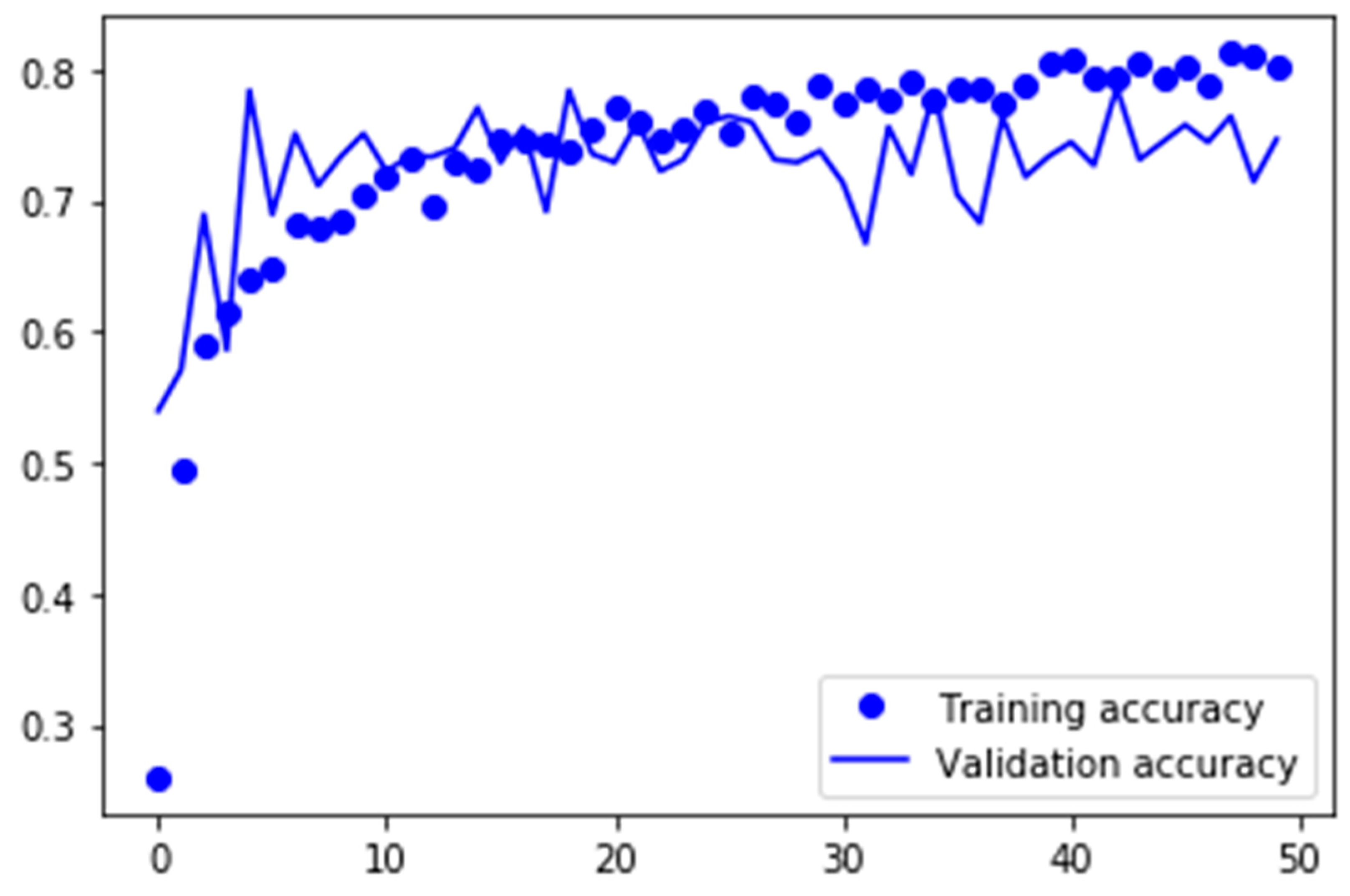
The evaluation of the second transfer learning approach with GoogLeNet is plotted in
Figure 19. Here the validation accuracy of the first epoch is worse compared with the transferred VGG-16, but with approximately 55%, it is still significantly better at the early stage than the previous models that classified the myFashion dataset. Here, the fluctuation of the validation accuracy is a little bit stronger than with VGG-16. A big fluctuation could indicate that some samples were guessed at some stages during training, and this may occur when important neurons are dropped because of dropout regularity.
The F1-score is a good metric to compare different classification models and looking at the F1-scores in
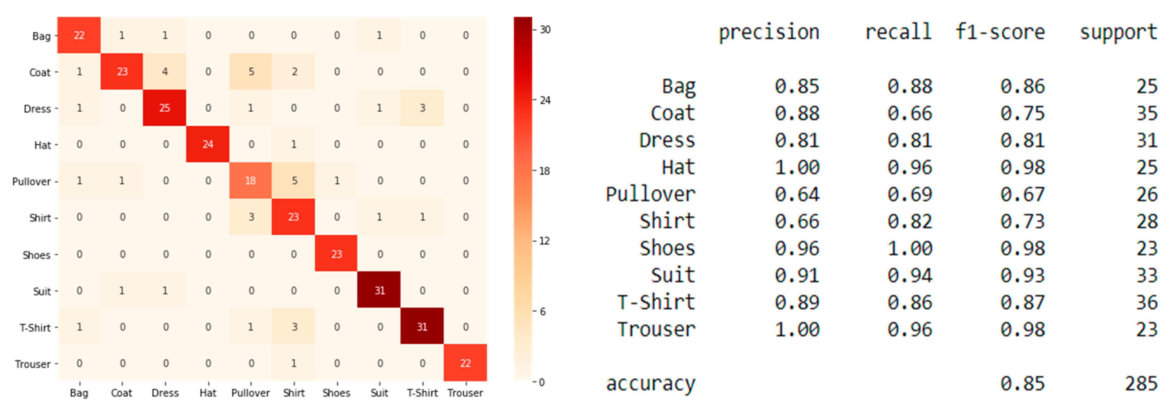
Table 7, it can be seen that the transferred VGG-16 achieved a better result than GoogLeNet. Therefore, the transferred VGG-16 classifier was further analyzed with the aid of the confusion matrix and classification report. Looking at the classification report in
Figure 20, it can be seen that with a precision of 1.00 none of the test images were wrongly classified as a hat or trousers; Furthermore, with an F1-score of just 0.67, the model classified pullovers the worst followed by shirts, with an F1-score of 0.73. The shoes, hat and trousers classes reached a remarkable F1-score of 0.98 and hence were the classes that were classified the best. The confusion matrix on the left shows, among other classes, that 24 out of the 25 hats in the test set were classified correctly, the other one was wrongly classified as shirt.
With an F1-score of 0.85, the transferred VGG-16 also outperformed model 2.2, which was implemented without transfer learning in
Section 5.2. This result means that in relation to the models’ performances, transfer learning was successful for this case study. Using the transferred knowledge of VGG-16, it was possible to further improve the F1-score from 0.78 up to 0.85, as well as improve the validation accuracy from 79% to a final 83%. On the other hand, this time, the training time suffered from the applied transfer learning. Training the transferred VGG-16 took about 45 min longer than in model 2.2 solely.
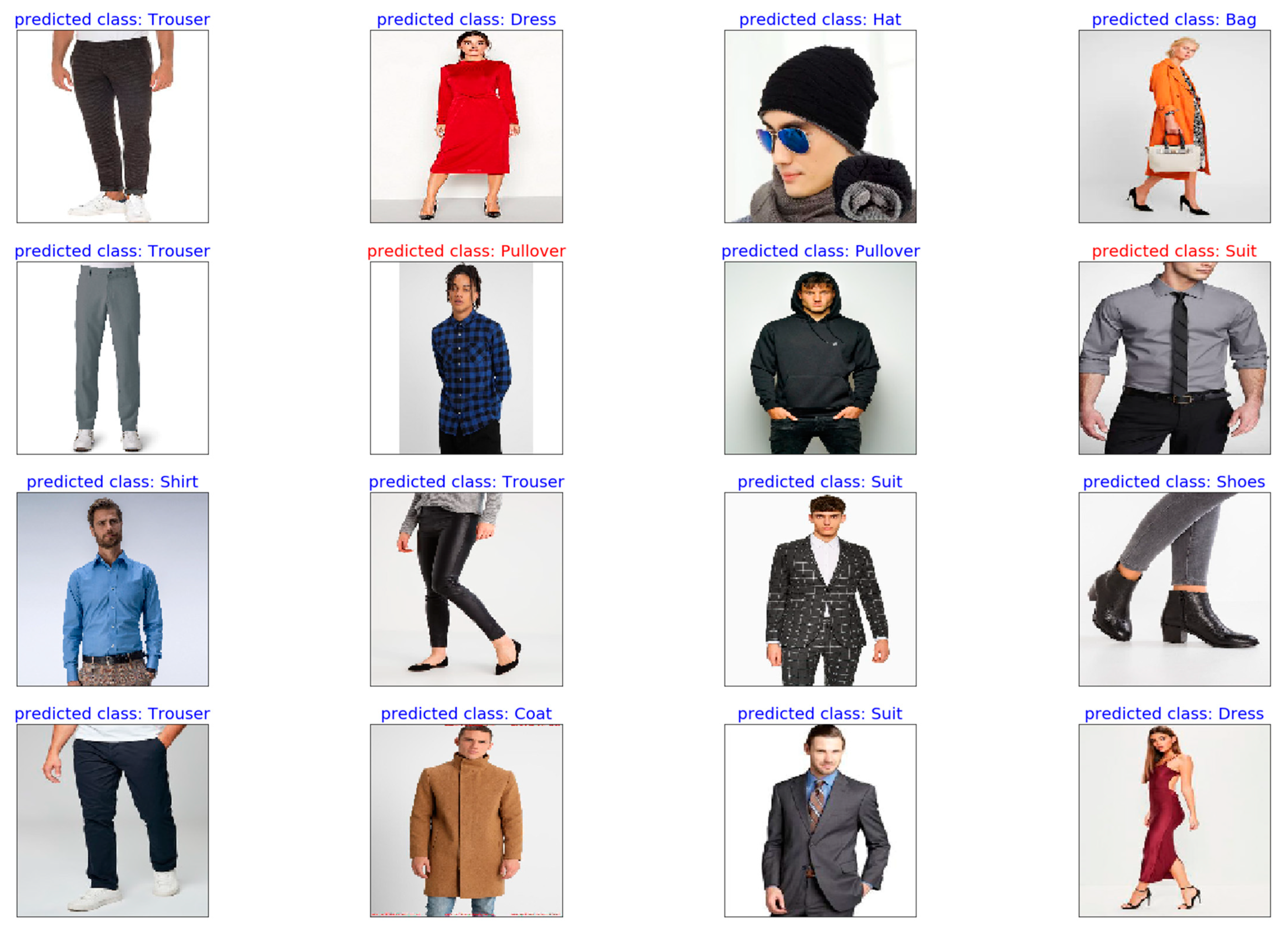
In a final step, to visualize the results, 16 test images were plotted together with their predicted labels in
Figure 21. In the plot, 14 out of the 16 test images were predicted correctly. The image in the fourth column in the second row was wrongly classified as a suit when it was a shirt. The image had some similarities to a suit outfit, especially because of the tie. The prediction could indicate that the model associated a shirt and tie combination with a suit. Principally, it can be said that the model had problems with the classification of long-sleeved apparel, like coats and pullovers. In general, upper body parts were classified worse than more distinct classes like trousers, shoes or hats.
6. Discussion
Research in apparel classification is increasing, but previous research mostly focused on recognizing and segmenting fashion article images solely without humans wearing the articles (e.g., for market basket analysis). To date, apparel classification mostly found application in criminal law, e-commerce or social media advertising [
25]. This article focused on classifying human-worn fashion images. The resulting model can be used for many different e-commerce applications. One of them is to automatically add links to social media posts, which lead to an online shop that directly shows all articles of the extracted apparel from the social media post.
To the authors, it was surprising at first that the state of the art for image classification was that one-sided. Almost all researchers in the novel literature are using TensorFlow to implement their convolutional neural network for image classification problems. Anaconda and Keras are not essential but make it much easier and convenient to build classification models.
The results of this article show that choosing the right CNN architecture is a complex task to do. Minor changes in the architecture can lead to big changes in the models’ performances, and just by changing the number of neurons or layers, a vast number of different architectures can be built [
30]. For this article, an architecture comprising three convolutional and three fully connected layers was defined. This architecture achieved an initial validation accuracy of 69.74% but was improved to 71.04% just by adding dropout regularity to the model. The validation accuracy further improved to 79.16% when data augmentation was used for preprocessing the data. Furthermore, for this dataset, applying dropout alone was not enough to prevent the model from overfitting, which only vanished when dropout and data augmentation were used together. The reason why data augmentation works so well on small datasets is through flipping, shifting and rotating, as well as zooming the training images, a bunch of new fake data is created and prevents the network from learning irrelevant features for the respective classes. Due to its success, data augmentation was also used for transfer learning. Transfer learning was used with the pretrained weights on ImageNet, which contains human-worn fashion images. With a validation accuracy of 83.96%, the VGG-16 dataset outperformed GoogLeNet, which only achieved a validation accuracy of 76.63%. In general, fine-tuning the transferred model improved the performance as well, but as the new dataset was small, it would more likely result in overfitting rather than in a performance improvement. Both models were trained with their respective preprocessing functions and the same training parameters. Hence, it can be assumed that the VGG-16 dataset was more suited to classify human-worn fashion images than GoogLeNet.
Compared with the transferred VGG-16 dataset, we can see that model 2.3 had more problems with classifying upper body parts. This can be interpreted as all upper body clothes entail similar characteristics and since model 2.2 was trained exclusively on the created dataset, the size may not have been large enough for the model to better distinguish between upper body clothes. The transferred VGG-16 dataset was pretrained with ImageNet, and hence it had much more data to learn more robust features for classification.
This article showed that for transfer learning, it is crucial that sufficient analogy between the source and target dataset exists. The analogy between fashion product images and human-worn fashion images was not sufficient, as the performance dropped significantly when the knowledge from the fashion MNIST dataset was used to predict human-worn fashion images. Therefore, the fashion MNIST dataset should rather be used for benchmarking prototypes.
The goal of this article was to implement an image classification model that extracted features from human-worn fashion images. This goal was achieved with the help of transfer learning using the VGG-16 dataset as a base model, with a final validation accuracy of 83.96% and a final F1-score of 0.85.
7. Conclusions
The aim of this article was to implement an image classification model to extract features from human-worn fashion images in small datasets. For this, the related literature was reviewed until the state of the art for image classification was sufficiently elaborated. It was found that convolutional neural networks were the undisputed standard for image classification tasks, and that they were most often implemented in an Anaconda environment with TensorFlow as the backend. Furthermore, methods like dropout regularity, data augmentation and transfer learning should be used when dealing with small datasets, as they can prevent against overfitting and improve the model’s generalization.
For the practical part, a human-worn fashion dataset with 2567 images was created. To see if and how the performance of a classification model that was trained on a small dataset could be improved, four approaches were defined and implemented in the course of this article. On the benchmark fashion MNIST dataset, dropout successfully prevented the model from overfitting and, in addition, was able to slightly improve the accuracy by 2% to a final validation accuracy of 94.02%. The second approach classified the created myFashion dataset solely. Here, the influence of data augmentation was tested. It showed that data augmentation not only prevented the model from overfitting, but it also improved the validation accuracy by 8% to 79.16% and the F1-score from 0.68 to 0.78. The third approach aimed to make use of the knowledge gained in approach one. However, the fashion MNIST dataset, consisting of Zalando product images, was not suited for classifying human-worn fashion images and resulted in a low F1-score of just 0.38 and a validation accuracy of 63.12%. In the fourth and last approach, transfer learning was performed on the VGG-16 and GoogLeNet datasets, loading their pretrained weights from ImageNet. With an F1-score of 0.85, the VGG-16 dataset outperformed GoogLeNet, which only achieved an F1-score of 0.72. The model predicted more distinct classes like hats, shoes and trousers the best and long-sleeved upper body clothes like coats and pullovers the worst.
To summarize, dropout prevented the model from overfitting, but only had a minor impact on the performance. Data augmentation could be used to enlarge the dataset with fake data and successfully prevented the model from overfitting and significantly improved the performance of the model. Data augmentation is vital when dealing with small datasets. Lastly, transfer learning showed that it is crucial that sufficient analogy between the source and the target dataset exists. The analogy between fashion product images and human-worn fashion images was not sufficient, as the performance dropped significantly when the knowledge from the fashion MNIST dataset was transferred.


