
An Enhancing Differential Evolution Algorithm with a Rank-Up Selection: RUSDE

Abstract
:1. Introduction
2. Related Works
2.1. Differential Evolution
2.2. Differential Evolution Variants
| Algorithm 1 The pseudo code of DE/rand/1 |
| Initialize a population X(N*D); Maximum iteration number MaxDT; for G = 1 to MaxDT do for i = 1 to N do Randomly select xa, xb, xc from the population X; Generate vi by Equation (1); for d = 1 to D do Generate ui by Equation (2); end for d end for i for i = 1 to N do Compute the fitness of ; if then Replace xi with ; end if end for i end for G |
3. The Proposed Methods
| Algorithm 2 The pseudo code of RUSDE |
| Initialize a population X(N*D); Maximum iteration number MaxDT, size of archive and let count = 0, flagrank = zeros(N,1), rankupvalue = zeros(N,MaxDT);Sort all individuals and calculate the current rank rankvalue(i,1) of ith individual. The first M individuals are stored into archive Y. for G = 2 to MaxDT do Sort all individuals in terms of fitness values; Record rank index of the ith individual in rankvalue(i, G) Calculate the rank-up value rankvalue(i, G) of ith individual by Equation (4) for i = 1 to N do if rankvalue(i, G) < 0(% individual’s rank up) then count = count + 1; index = mod(count,M); Y(index,:) = x(i,:)(%Store this individual into Y, and replace the earliest one); flagrank(i) = 0; else flagrank(i) = flagrank(i) + 1; end if end for i for i = 1 to N do Randomly select X1, X2, X3 from the population X and Y1, Y2, Y3 from the archive Y; Generate vi by Equation (7); for d = 1 to D do Generate vi by Equation (9); end for d end for i for i = 1 to N do Compute the fitness of ; if then Replace xi with ; if then ; flagbest = 0; else flagbest = flagbest + 1; end if end if end for i end for G |
4. Experiments
4.1. Benchmarks and Experimental Settings
4.2. The Influence of Parameter M
4.3. Comparisons with Other Algorithms and Statistical Analysis of The Results
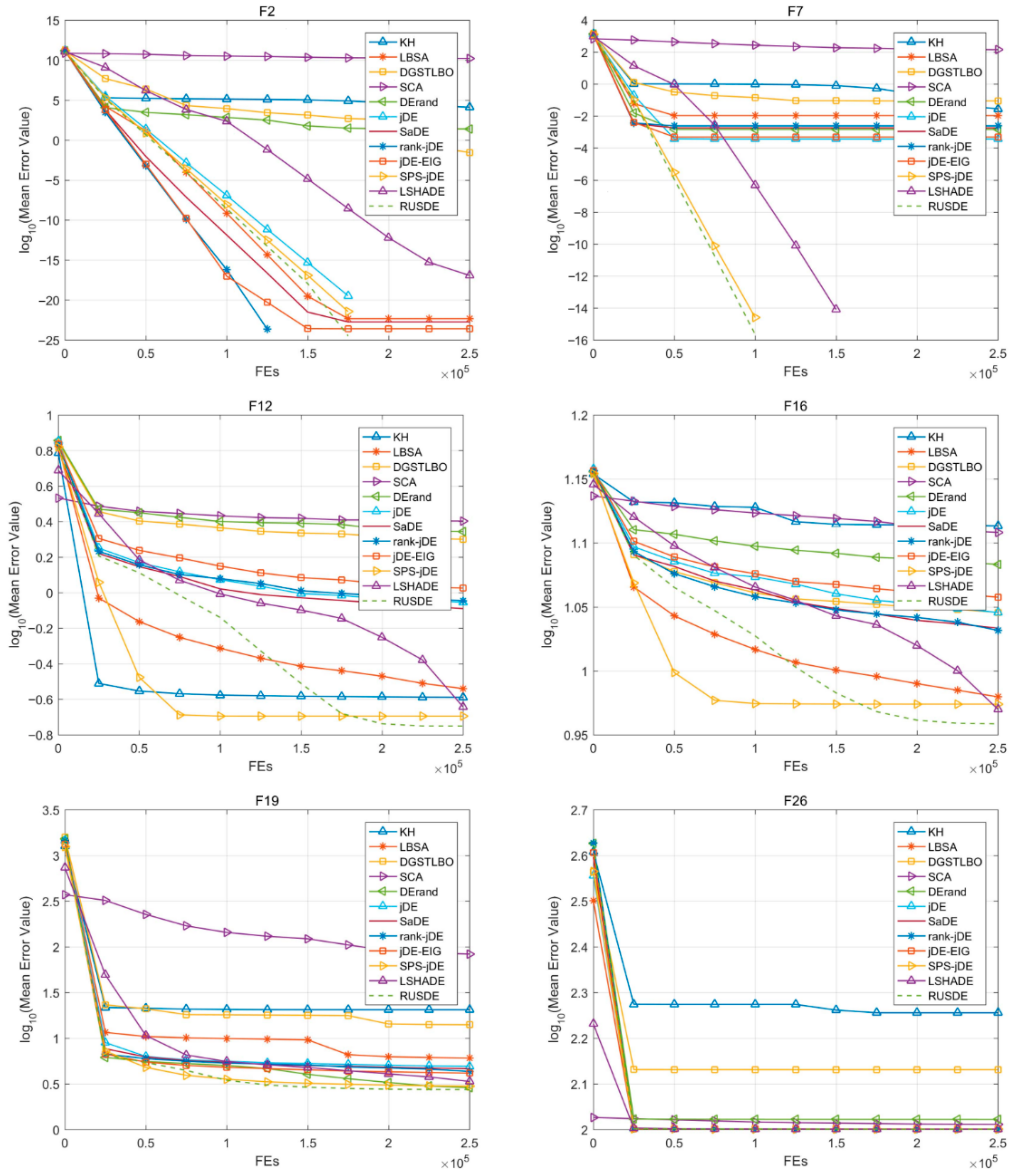
4.4. Convergence Performance of RUSDE
5. Application Example
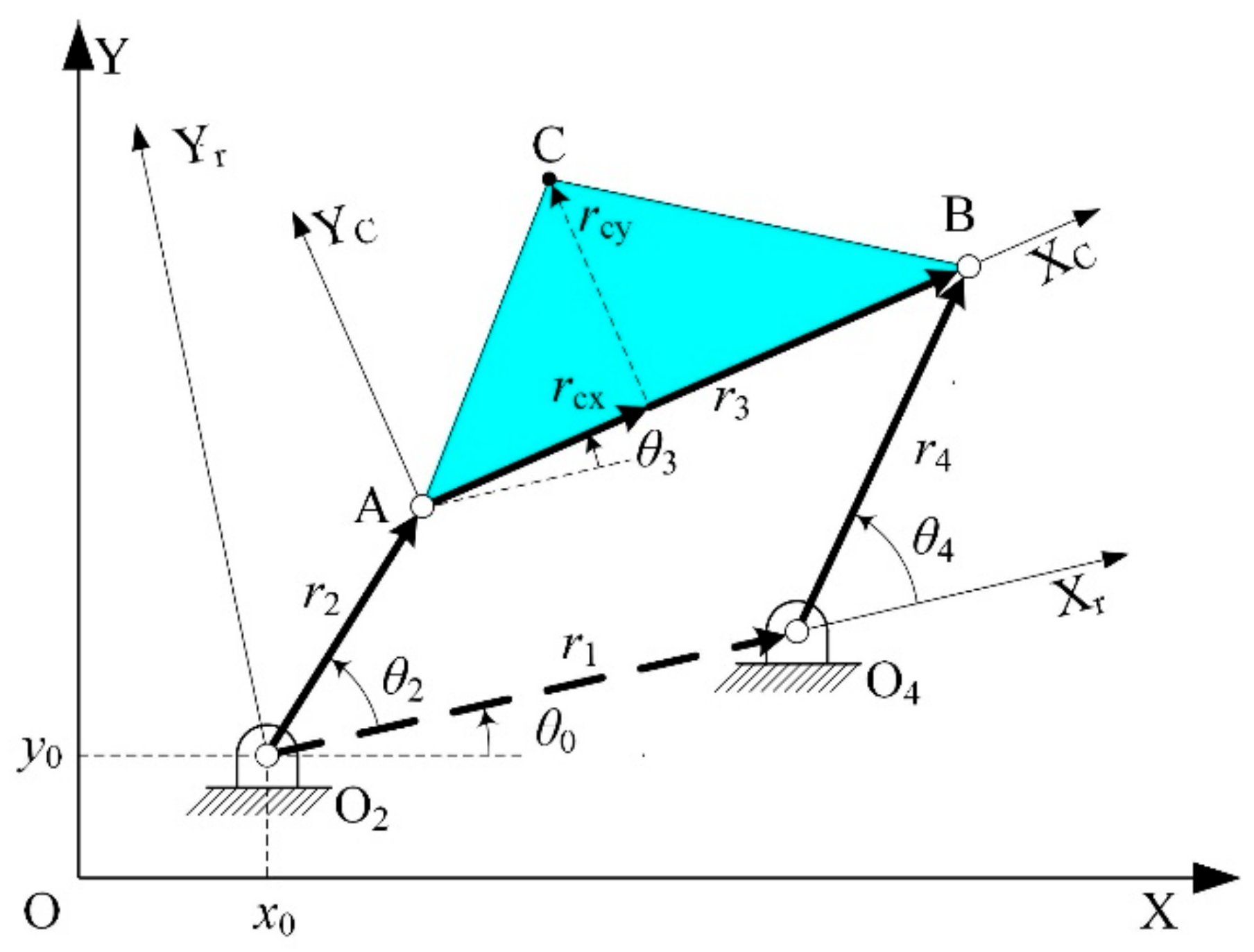
5.1. The Classic Case of Four-Bar Mechanism
5.2. The Constraints and Goal Function
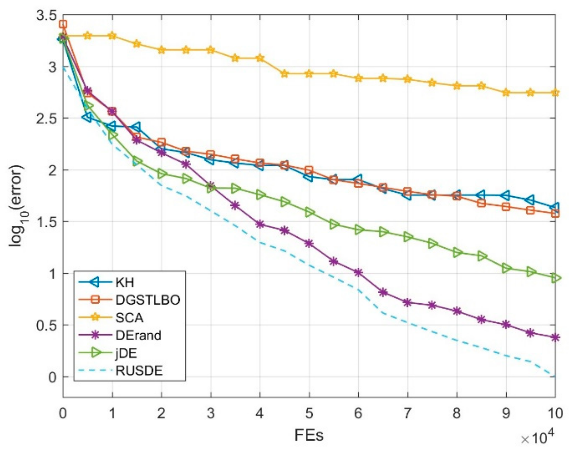
5.3. The Experimental Settings and Results
6. Conclusions
Author Contributions
Funding
Conflicts of Interest
Appendix A

| No. | Function Name | Expression | Fi* |
|---|---|---|---|
| F1 | Rotated High Conditioned Elliptic Function | 100 | |
| F2 | Rotated Bent Cigar Function | 200 | |
| F3 | Rotated Discus Function | 300 | |
| F4 | Shifted and Rotated Rosenbrock’s Function | 400 | |
| F5 | Shifted and Rotated Ackley’s Function | 500 | |
| F6 | Shifted and Rotated Weierstrass Function | 600 | |
| F7 | Shifted and Rotated Griewank’s Function | 700 | |
| F8 | Shifted Rastrigin’s Function | 800 | |
| F9 | Shifted and Rotated Rastrigin’s Function | 900 | |
| F10 | Shifted Schwefel’s Function | 1000 | |
| F11 | Shifted and Rotated Schwefel’s Function | 1100 | |
| F12 | Shifted and Rotated Katsuura Function | 1200 | |
| F13 | Shifted and Rotated HappyCat Function | 1300 | |
| F14 | Shifted and Rotated HGBat Function | 1400 | |
| F15 | Shifted and Rotated Expanded Griewank’s plus Rosenbrock’s Function | 1500 | |
| F16 | Shifted and Rotated Expanded Scaffer’s F6 Function | 1600 | |
where | |||
| F17 | Hybrid Function 1 | N = 3, p = [0.3, 0.3, 0.4], g = [] | 1700 |
| F18 | Hybrid Function 2 | N = 3, p = [0.3, 0.3, 0.4], g = [] | 1800 |
| F19 | Hybrid Function 3 | N = 4, p = [0.2, 0.2, 0.3, 0.3], g = | 1900 |
| F20 | Hybrid Function 4 | N = 4, p = [0.2, 0.2, 0.3, 0.3], g = | 2000 |
| F21 | Hybrid Function 5 | N = 5, p = [0.1, 0.2, 0.2, 0.2 0.3], g = | 2100 |
| F22 | Hybrid Function 6 | N = 5, p = [0.1, 0.2, 0.2, 0.2 0.3], g = | 2200 |
| F23 | Composition Function 1 | bias = [0, 100, 200, 300, 400], g = [F4′, F1′, F2′, F3′, F1′] | 2300 |
| F24 | Composition Function 2 | N = 3, σ = [20, 20, 20], λ = [1, 1, 1], bias = [0, 100, 200], g = [F10′, F9′, F11′] | 2400 |
| F25 | Composition Function 3 | bias = [0, 100, 200], g = [F11′, F9′, F1′] | 2500 |
| F26 | Composition Function 4 | bias = [0, 100, 200, 300, 400], g = [F11′, F13′, F1′, F6′, F7′] | 2600 |
| F27 | Composition Function 5 | bias = [0, 100, 200, 300, 400], g = [F14′, F9′, F11′, F6′, F1′] | 2700 |
| F28 | Composition Function 6 | bias = [0, 100, 200, 300, 400], g = [F15′, F13′, F11′, F16′, F1′] | 2800 |
| F29 | Composition Function 7 | N = 3, σ = [10, 30, 50], λ = [1, 1, 1], bias = [0, 100, 200], g = [F17′, F18′’, F19′] | 2900 |
| F30 | Composition Function 8 | N = 3, σ = [10, 30, 50], λ = [1, 1, 1], bias = [0, 100, 200], g = [F20′, F21′, F22′] | 3000 |
| No. | Function Name | Expression |
|---|---|---|
| F1 | High Conditioned Elliptic Function | |
| F2 | Bent Cigar Function | |
| F3 | Discus Function | |
| F4 | Rosenbrock’s Function | |
| F5 | Ackley’s Function | |
| F6 | Weierstrass Function | where a = 0.5, b = 3, kmax = 20 |
| F7 | Griewank’s Function | |
| F8 | Rastrigin’s Function | |
| F9 | Modified Schwefel’s Function | where |
| F10 | Katsuura Function | |
| F11 | HappyCat Function | |
| F12 | HGBat Function | |
| F13 | Expanded Griewank’s plus Rosenbrock’s Function | |
| F14 | Expanded Scaffer’s F6 Function |
References
- Holland, J. Adaptation in Natural and Artificial Systems: An Introductory Analysis with Application to Biology. Control and Artificial Intelligence; MIT Press: Cambridge, MA, USA, 1975. [Google Scholar]
- Dorigo, M. Optimization, Learning and Natural Algorithms. Ph.D. Thesis, Politecnico di Milano, Milan, Italy, 1992. [Google Scholar]
- Kennedy, J.; Eberhart, R. Particle swarm optimization. In Proceedings of the IEEE International Conference on Neural Networks—Conference Proceedings, Perth, WA, Australia, 27 November–1 December 1995. [Google Scholar]
- Xin-She, Y.; Deb, S. Cuckoo search via Lévy flights. In Proceedings of the 2009 World Congress on Nature & Biologically Inspired Computing (NaBIC), Coimbatore, India, 9–11 December 2009. [Google Scholar]
- Rao, R.; Savsani, V.; Vakharia, D. Teaching–learning-based optimization: A novel method for constrained mechanical design optimization problems. Comput. Des. 2011, 43, 303–315. [Google Scholar] [CrossRef]
- Črepinšek, M.; Liu, S.-H.; Mernik, L. A note on teaching–learning-based optimization algorithm. Inf. Sci. 2012, 212, 79–93. [Google Scholar] [CrossRef]
- Črepinšek, M.; Liu, S.-H.; Mernik, L.; Mernik, M. Is a comparison of results meaningful from the inexact replications of computational experiments? Soft Comput. 2016, 20, 223–235. [Google Scholar] [CrossRef] [Green Version]
- Gandomi, A.H.; Alavi, A.H. Krill herd: A new bio-inspired optimization algorithm. Commun. Nonlinear Sci. Numer. Simul. 2012, 17, 4831–4845. [Google Scholar] [CrossRef]
- Civicioglu, P. Backtracking Search Optimization Algorithm for numerical optimization problems. Appl. Math. Comput. 2013, 219, 8121–8144. [Google Scholar] [CrossRef]
- Rainer, S.; Price, K. Differential evolution—A simple and efficient heuristic for global optimization over con-tinuous spaces. J. Glob. Optim. 1997, 11, 341–359. [Google Scholar]
- García, S.; Molina, D.; Lozano, M.; Herrera, F. A study on the use of non-parametric tests for analyzing the evolutionary algorithms’ behaviour: A case study on the CEC’2005 Special Session on Real Parameter Optimization. J. Heuristics 2009, 15, 617–644. [Google Scholar] [CrossRef]
- Derrac, J.; García, S.; Molina, D.; Herrera, F. A practical tutorial on the use of nonparametric statistical tests as a methodology for comparing evo-lutionary and swarm intelligence algorithms. Swarm Evol. Comput. 2011, 1, 3–18. [Google Scholar] [CrossRef]
- Pan, Z.; Liang, H.; Gao, Z.; Gao, J. Differential evolution with subpopulations for high-dimensional seismic inversion. Geophys. Prospect. 2018, 66, 1060–1069. [Google Scholar] [CrossRef] [Green Version]
- Elferik, S.; Hassan, M.; Alnaser, M. Adaptive Valve Stiction Compensation Using Differential Evolution. J. Chem. Eng. Jpn. 2018, 51, 407–417. [Google Scholar] [CrossRef]
- Qiu, X.; Xu, J.-X.; Xu, Y.H.; Tan, K.C. A New Differential Evolution Algorithm for Minimax Optimization in Robust Design. IEEE Trans. Cybern. 2018, 48, 1355–1368. [Google Scholar] [CrossRef] [PubMed]
- Aguitoni, M.C.; Pavão, L.V.; Siqueira, P.H.; Jiménez, L.; Ravagnani, M.A.D.S.S. Heat exchanger network synthesis using genetic algorithm and differential evolution. Comput. Chem. Eng. 2018, 117, 82–96. [Google Scholar] [CrossRef]
- Ak, C.; Yildiz, A.; Yıldız, A. A Novel Closed-Form Expression Obtained by Using Differential Evolution Algorithm to Calculate Pull-In Voltage of MEMS Cantilever. J. Microelectromech. Syst. 2018, 27, 392–397. [Google Scholar] [CrossRef]
- Zhao, W.-J.; Liu, E.-X.; Wang, B.; Gao, S.-P.; Png, C.E. Differential Evolutionary Optimization of an Equivalent Dipole Model for Electromagnetic Emission Analysis. IEEE Trans. Electromagn. Compat. 2018, 60, 1635–1639. [Google Scholar] [CrossRef]
- Manjit, K.; Kumar, V. Colour image encryption technique using differential evolution in non-subsampled con-tourlet transform domain. IET Image Process. 2018, 12, 1273–1283. [Google Scholar]
- Zhou, Z.; Gao, X.; Zhang, J.; Zhu, Z.; Hu, X. A novel hybrid model using the rotation forest-based differential evolution online sequential extreme learning machine for illumination correction of dyed fabrics. Text. Res. J. 2019, 89, 1180–1197. [Google Scholar] [CrossRef]
- Wang, Y.; Zhou, M.; Song, X.; Gu, M.; Sun, J. Constructing Cost-Aware Functional Test-Suites Using Nested Differential Evolution Algorithm. IEEE Trans. Evol. Comput. 2017, 22, 334–346. [Google Scholar] [CrossRef]
- Wang, L.; Zeng, Y.; Chen, T. Back propagation neural network with adaptive differential evolution algorithm for time series forecasting. Expert Syst. Appl. 2015, 42, 855–863. [Google Scholar] [CrossRef]
- Marco, B.; Milani, A.; Santucci, V. Learning bayesian networks with algebraic differential evolution. In Proceedings of the International Conference on Parallel Problem Solving from Nature, Coimbra, Portugal, 8–12 September 2018. [Google Scholar]
- Aleš, Z.; Sosa, J.D.H. Success history applied to expert system for underwater glider path planning using differential evolution. Expert Syst. Appl. 2019, 119, 155–170. [Google Scholar]
- Qin, A.K.; Huang, V.L.; Suganthan, P.N. Differential Evolution Algorithm with Strategy Adaptation for Global Numerical Optimization. IEEE Trans. Evol. Comput. 2008, 13, 398–417. [Google Scholar] [CrossRef]
- Brest, J.; Greiner, S.; Boskovic, B.; Mernik, M.; Zumer, V. Self-Adapting Control Parameters in Differential Evolution: A Comparative Study on Numerical Benchmark Problems. IEEE Trans. Evol. Comput. 2006, 10, 646–657. [Google Scholar] [CrossRef]
- Zhang, J.; Sanderson, A.C. JADE: Adaptive Differential Evolution with Optional External Archive. IEEE Trans. Evol. Comput. 2009, 13, 945–958. [Google Scholar] [CrossRef]
- Ryoji, T.; Fukunaga, A. Success-history based parameter adaptation for differential evolution. In Proceedings of the 2013 IEEE Congress on Evolutionary Computation, Cancun, Mexico, 20–23 June 2013. [Google Scholar]
- Guo, S.-M.; Yang, C.-C.; Hsu, P.-H.; Tsai, J.S.H. Improving Differential Evolution with a Successful-Parent-Selecting Framework. IEEE Trans. Evol. Comput. 2015, 19, 717–730. [Google Scholar] [CrossRef]
- Guo, S.-M.; Yang, C.-C. Enhancing Differential Evolution Utilizing Eigenvector-Based Crossover Operator. IEEE Trans. Evol. Comput. 2015, 19, 31–49. [Google Scholar] [CrossRef]
- Gong, W.; Cai, Z. Differential Evolution with Ranking-Based Mutation Operators. IEEE Trans. Cybern. 2013, 43, 2066–2081. [Google Scholar] [CrossRef] [PubMed]
- Guo, L.; Li, X.; Gong, W. Ranking-Based Differential Evolution for Large-Scale Continuous Optimization. Comput. Inform. 2018, 37, 49–75. [Google Scholar] [CrossRef]
- Tang, L.; Dong, Y.; Liu, J. Differential Evolution with an Individual-Dependent Mechanism. IEEE Trans. Evol. Comput. 2014, 19, 560–574. [Google Scholar] [CrossRef] [Green Version]
- Das, S.; Abraham, A.; Chakraborty, U.K.; Konar, A. Differential Evolution Using a Neighborhood-Based Mutation Operator. IEEE Trans. Evol. Comput. 2009, 13, 526–553. [Google Scholar] [CrossRef] [Green Version]
- Mallipeddi, R.; Suganthan, P.; Pan, Q.; Tasgetiren, M. Differential evolution algorithm with ensemble of parameters and mutation strategies. Appl. Soft Comput. 2011, 11, 1679–1696. [Google Scholar] [CrossRef]
- Islam, S.M.; Das, S.; Ghosh, S.; Roy, S.; Suganthan, P.N. An Adaptive Differential Evolution Algorithm with Novel Mutation and Crossover Strategies for Global Numerical Optimization. IEEE Trans. Syst. Man Cybern. Part B Cybern. 2012, 42, 482–500. [Google Scholar] [CrossRef]
- Segredo, E.; Lalla-Ruiz, E.; Hart, E. A novel similarity-based mutant vector generation strategy for differential evolution. In Proceedings of the Genetic and Evolutionary Computation Conference, Kyoto, Japan, 15–19 July 2018. [Google Scholar]
- Xu, B.; Tao, L.; Chen, X.; Cheng, W. Adaptive differential evolution with multi-population-based mutation operators for constrained optimization. Soft Comput. 2019, 23, 3423–3447. [Google Scholar] [CrossRef]
- Peng, H.; Guo, Z.; Deng, C.; Wu, Z. Enhancing differential evolution with random neighbors based strategy. J. Comput. Sci. 2018, 26, 501–511. [Google Scholar] [CrossRef]
- Huang, Q.; Zhang, K.; Song, J.; Zhang, Y.; Shi, J. Adaptive differential evolution with a Lagrange interpolation argument algorithm. Inf. Sci. 2019, 472, 180–202. [Google Scholar] [CrossRef]
- Liang, J.; Qu, B.Y.; Suganthan, P.N. Problem definitions and evaluation criteria for the CEC 2014 special session and competition on single objective real-parameter numerical optimization. In Computational Intelligence Laboratory, Zhengzhou University, Zhengzhou China and Technical Report; Nanyang Technological University: Singapore, 2013; p. 635. [Google Scholar]
- Rahnamayan, S.; Tizhoosh, H.R.; Salama, M.M.A. Opposition-Based Differential Evolution. IEEE Trans. Evol. Comput. 2008, 12, 64–79. [Google Scholar] [CrossRef] [Green Version]
- Wang, H.; Wu, Z.; Rahnamayan, S. Enhanced opposition-based differential evolution for solving high-dimensional continuous optimization problems. Soft Comput. 2010, 15, 2127–2140. [Google Scholar] [CrossRef]
- Hansen, N.; Ostermeier, A. Completely Derandomized Self-Adaptation in Evolution Strategies. Evol. Comput. 2001, 9, 159–195. [Google Scholar] [CrossRef]
- Hansen, N.; Niederberger, A.S.P.; Guzzella, L.; Koumoutsakos, P. A Method for Handling Uncertainty in Evolutionary Optimization with an Application to Feedback Control of Combustion. IEEE Trans. Evol. Comput. 2008, 13, 180–197. [Google Scholar] [CrossRef]
- Ghosh, S.; Das, S.; Roy, S.; Islam, S.M.; Suganthan, P. A Differential Covariance Matrix Adaptation Evolutionary Algorithm for real parameter optimization. Inf. Sci. 2012, 182, 199–219. [Google Scholar] [CrossRef]
- Wang, Y.; Li, H.-X.; Huang, T.; Li, L. Differential evolution based on covariance matrix learning and bimodal distribution parameter setting. Appl. Soft Comput. 2014, 18, 232–247. [Google Scholar] [CrossRef]
- Wang, Y.; Cai, Z.; Zhang, Q. Enhancing the search ability of differential evolution through orthogonal crossover. Inf. Sci. 2012, 185, 153–177. [Google Scholar] [CrossRef]
- Wang, H.; Rahnamayan, S.; Sun, H.; Omran, M.G.H. Gaussian Bare-Bones Differential Evolution. IEEE Trans. Cybern. 2013, 43, 634–647. [Google Scholar] [CrossRef] [PubMed]
- Wang, Y.; Cai, Z.; Zhang, Q. Differential Evolution with Composite Trial Vector Generation Strategies and Control Parameters. IEEE Trans. Evol. Comput. 2011, 15, 55–66. [Google Scholar] [CrossRef]
- Dorronsoro, B.; Bouvry, P. Improving Classical and Decentralized Differential Evolution with New Mutation Operator and Population Topologies. IEEE Trans. Evol. Comput. 2011, 15, 67–98. [Google Scholar] [CrossRef]
- Črepinšek, M.; Liu, S.-H.; Mernik, M.; Ravber, M. Long Term Memory Assistance for Evolutionary Algorithms. Mathematics 2019, 7, 1129. [Google Scholar] [CrossRef] [Green Version]
- Auger, A.; Hansen, N. A restart CMA evolution strategy with increasing population size. In Proceedings of the 2005 IEEE Congress on Evolutionary Computation, Scotland, UK, 2–5 September 2005; Volume 2, pp. 1769–1776. [Google Scholar]
- Brest, J.; Maučec, M.S.; Bošković, B. Single objective real-parameter optimization: Algorithm jSO. In Proceedings of the 2017 IEEE Congress on Evolutionary Computation (CEC), San Sebastián, Spain, 5–8 June 2017; pp. 1311–1318. [Google Scholar]
- Cai, Y.; Wang, J. Differential evolution with neighborhood and direction information for numerical optimiza-tion. IEEE Trans. Cybern. 2013, 43, 2202–2215. [Google Scholar] [CrossRef]
- Brest, J.; Korosec, P.; Šilc, J.; Zamuda, A.; Bošković, B.; Maučec, M.S. Differential evolution and differential ant-stigmergy on dynamic optimisation problems. Int. J. Syst. Sci. 2013, 44, 663–679. [Google Scholar] [CrossRef]
- Zhang, K.; Huang, Q.; Zhang, Y. Enhancing comprehensive learning particle swarm optimization with local optima topology. Inf. Sci. 2019, 471, 1–18. [Google Scholar] [CrossRef]
- Salomon, R. Re-evaluating genetic algorithm performance under coordinate rotation of benchmark functions. A survey of some theoretical and practical aspects of genetic algorithms. BioSystems 1996, 39, 263–278. [Google Scholar] [CrossRef]
- Tanabe, R.; Fukunaga, A.S. Improving the search performance of SHADE using linear population size reduction. In Proceedings of the 2014 IEEE Congress on Evolutionary Computation (CEC), Beijing, China, 6–11 July 2014. [Google Scholar]
- Chen, D.; Zou, F.; Lu, R.; Wang, P. Learning backtracking search optimisation algorithm and its application. Inf. Sci. 2017, 376, 71–94. [Google Scholar] [CrossRef]
- Zou, F.; Wang, L.; Hei, X.; Chen, D.; Yang, D. Teaching–learning-based optimization with dynamic group strategy for global optimization. Inf. Sci. 2014, 273, 112–131. [Google Scholar] [CrossRef]
- Mirjalili, S. SCA: A Sine Cosine Algorithm for solving optimization problems. Knowl. Based Syst. 2016, 96, 120–133. [Google Scholar] [CrossRef]
- Veček, N.; Črepinšek, M.; Mernik, M. On the influence of the number of algorithms, problems, and independent runs in the comparison of evolutionary algorithms. Appl. Soft Comput. 2017, 54, 23–45. [Google Scholar] [CrossRef]
- Singh, R.; Chaudhary, H.; Singh, A.K. Defect-free optimal synthesis of crank-rocker linkage using nature-inspired optimization algorithms. Mech. Mach. Theory 2017, 116, 105–122. [Google Scholar] [CrossRef]


| Func. | A1. | M = 20 | M = 40 | M = 50 | M = 60 | M = 80 | M = 100 |
|---|---|---|---|---|---|---|---|
| F1 | Mean | 2.94 × 10⁵ | 5.10 × 10⁵ | 3.96 × 10⁶ | 4.01 × 10⁶ | 5.00 × 10⁶ | 3.43 × 10⁶ |
| F2 | Mean | 1.24 × 10⁻⁹ | 2.19 × 10⁻⁸ | 4.35 × 10⁻¹⁰ | 1.76 × 10⁻⁸ | 2.95 × 10⁻⁷ | 1.84 × 10⁻⁶ |
| F3 | Mean | 3.48 × 10⁻¹⁰ | 5.47 × 10⁻⁹ | 1.04 × 10⁻¹³ | 9.74 × 10⁻¹⁶ | 1.92 × 10⁻¹⁵ | 2.03 × 10⁻⁵ |
| F4 | Mean | 11.5 | 25.2 | 8.11 | 1.70 | 19 | 9.05 |
| F5 | Mean | 20.6 | 20.6 | 20.4 | 20.4 | 20.4 | 20.3 |
| F6 | Mean | 0.142 | 4.19 × 10⁻⁴ | 0.135 | 12.3 | 14.4 | 14.3 |
| F7 | Mean | 0.00 | 7.40 × 10⁻⁴ | 0.00 | 0.00 | 0.00 | 1.11 × 10⁻¹⁷ |
| F8 | Mean | 0.00000011 | 0.0000358 | 6.16 × 10⁻¹⁰ | 4.41 × 10⁻¹⁰ | 1.52 × 10⁻⁹ | 1.7 × 10⁻⁹ |
| F9 | Mean | 33.6 | 58.6 | 49.1 | 52.1 | 53.0 | 54.8 |
| F10 | Mean | 40.8 | 59.8 | 4.91 × 10⁻³ | 5.78 × 10⁻³ | 6.90 × 10⁻³ | 1.61 × 10⁻² |
| F11 | Mean | 2.23 × 10³ | 4.16 × 10³ | 2.70 × 10³ | 2.74 × 10³ | 2.77 × 10³ | 2.73 × 10³ |
| F12 | Mean | 0.569 | 0.952 | 0.517 | 0.536 | 0.489 | 0.549 |
| F13 | Mean | 0.271 | 0.28 | 0.237 | 0.239 | 0.225 | 0.292 |
| F14 | Mean | 0.29 | 0.292 | 0.278 | 0.255 | 0.262 | 0.251 |
| F15 | Mean | 3.96 | 10.0 | 6.36 | 6.59 | 6.28 | 6.52 |
| F16 | Mean | 10.9 | 11.2 | 10.0 | 9.95 | 10.1 | 10.2 |
| F17 | Mean | 5.53 × 10⁻³ | 4.04 × 10³ | 1.29 × 10³ | 6.64 × 10² | 6.48 × 10² | 6.34 × 10² |
| F18 | Mean | 44.8 | 47.2 | 14.4 | 15.2 | 17.7 | 13.2 |
| F19 | Mean | 3.32 | 4.13 | 4.57 | 4.82 | 5.02 | 6.15 |
| F20 | Mean | 11.6 | 12.0 | 12.1 | 17.0 | 9.11 | 9.47 |
| F21 | Mean | 9.48 × 10² | 8.27 × 10² | 3.26 × 10² | 3.15 × 10² | 3.61 × 10² | 3.47 × 10² |
| F22 | Mean | 1.29 × 10² | 1.01 × 10² | 1.85 × 10² | 1.70 × 10² | 1.38 × 10² | 2.21 × 10² |
| F23 | Mean | 3.15 × 10² | 3.15 × 10² | 3.15 × 10² | 3.15 × 10² | 3.15 × 10² | 3.15 × 10² |
| F24 | Mean | 2.23 × 10² | 2.23 × 10² | 2.23 × 10² | 2.23 × 10² | 2.24 × 10² | 2.24 × 10² |
| F25 | Mean | 2.03 × 10² | 2.03 × 10² | 2.05 × 10² | 2.05 × 10² | 2.05 × 10² | 2.05 × 10² |
| F26 | Mean | 1.00 × 10² | 1.00 × 10² | 1.00 × 10² | 1.00 × 10² | 1.00 × 10² | 1.00 × 10² |
| F27 | Mean | 3.14 × 10² | 3.09 × 10² | 3.00 × 10² | 3.00 × 10² | 3.00 × 10² | 3.04 × 10² |
| F28 | Mean | 8.04 × 10² | 8.16 × 10² | 7.95 × 10² | 8.10 × 10² | 8.09 × 10² | 8.14 × 10² |
| F29 | Mean | 1.06 × 10³ | 9.73 × 10² | 9.58 × 10² | 7.95 × 10² | 8.00 × 10² | 1.30 × 10³ |
| F30 | Mean | 1.08 × 10³ | 1.29 × 10³ | 1.29 × 10³ | 1.40 × 10³ | 1.78 × 10³ | 1.87 × 10³ |
| Average Rank | 3.07 | 4.20 | 2.37 | 2.57 | 3.07 | 3.80 |
| Func. | A1. | KH | LBSA | DGSTLBO | SCA | DErand | jDE | SaDE | rank-jDE | jDE-EIG | SPS-jDE | LSHADE | RUSDE |
|---|---|---|---|---|---|---|---|---|---|---|---|---|---|
| F1 | Mean | 1.27 × 10⁶ | 1.20 × 10⁵ | 3.82 × 10⁵ | 2.54 × 10⁸ | 1.59 × 10⁵ | 6.87 × 10⁵ | 1.42 × 10⁴ | 1.00 × 10⁵ | 8.17 × 10⁴ | 1.77 × 10⁵ | 2.00 × 10² | 1.13 × 10⁵ |
| Std. | 4.16 × 10⁵ | 1.01 × 10⁵ | 2.11 × 10⁵ | 8.21 × 10⁷ | 1.72 × 10⁵ | 3.89 × 10⁵ | 1.40 × 10⁴ | 6.46 × 10⁴ | 8.81 × 10⁴ | 1.14 × 10⁵ | 1.60× 10⁻⁵ | 6.53 × 10⁴ | |
| F2 | Mean | 1.28 × 10⁴ | 4.65 × 10⁻²³ | 2.85 × 10⁻² | 1.65 × 10¹⁰ | 25.1 | 0.00 | 1.82 × 10⁻²³ | 0.00 | 2.52 × 10⁻²⁴ | 0.00 | 1.19 × 10⁻¹⁷ | 0.00 |
| Std. | 6.42 × 10³ | 1.03 × 10⁻²² | 0.115 | 2.49 × 10⁹ | 1.12 × 10² | 0.00 | 5.62 × 10⁻²³ | 0.00 | 1.13 × 10⁻²³ | 0.00 | 1.15 × 10⁻¹⁷ | 0.00 | |
| F3 | Mean | 3.83 × 10⁴ | 8.53 × 10⁻³⁰ | 3.96 × 10⁻⁴ | 3.73 × 10⁴ | 1.46 | 4.95 × 10⁻²⁵ | 4.77 × 10⁻²⁸ | 1.87 × 10⁻²⁹ | 1.25 × 10⁻²⁷ | 9.77 × 10⁻²⁸ | 2.13 × 10⁻²² | 3.08 × 10⁻²⁸ |
| Std. | 1.08 × 10⁴ | 2.37 × 10⁻²⁹ | 1.61 × 10⁻³ | 6.46 × 10³ | 3.97 | 6.89 × 10⁻²⁵ | 1.22 × 10⁻²⁷ | 4.28 × 10⁻²⁹ | 3.11 × 10⁻²⁷ | 1.92 × 10⁻²⁷ | 3.21 × 10⁻²² | 1.32 × 10⁻²⁷ | |
| F4 | Mean | 65.6 | 7.25 | 92.6 | 1.12 × 10³ | 21.0 | 0.566 | 0.343 | 6.04 × 10⁻³ | 0.106 | 4.10 | 0.557 | 0.403 |
| Std. | 37.2 | 20.7 | 27.4 | 3.08 × 10² | 37.8 | 0.295 | 0.22 | 1.63 × 10⁻² | 0.155 | 14.9 | 0.451 | 0.212 | |
| F5 | Mean | 20.0 | 20.2 | 20.9 | 20.9 | 21.0 | 20.5 | 20.6 | 20.5 | 20.6 | 20.4 | 20.2 | 20.4 |
| Std. | 6.45 × 10⁻⁴ | 3.45 × 10⁻² | 3.84 × 10⁻² | 5.29 × 10⁻² | 4.80 × 10⁻² | 4.42 × 10⁻² | 5.36 × 10⁻² | 4.58 × 10⁻² | 4.73 × 10⁻² | 0.116 | 3.83 × 10⁻² | 0.111 | |
| F6 | Mean | 20.5 | 7.06 | 20.8 | 34.4 | 0.663 | 0.361 | 0.806 | 1.33 | 0.593 | 0.581 | 10.3 | 0.432 |
| Std. | 3.28 | 1.87 | 2.70 | 2.59 | 1.00 | 0.765 | 1.49 | 1.08 | 0.881 | 0.72 | 0.815 | 0.82 | |
| F7 | Mean | 2.81 × 10⁻² | 1.08 × 10⁻² | 8.91 × 10⁻² | 1.43 × 10² | 1.48 × 10⁻² | 3.70 × 10⁻⁴ | 1.84 × 10⁻³ | 2.46 × 10⁻³ | 4.93 × 10⁻⁴ | 0.00 | 0.00 | 0.00 |
| Std. | 1.24 × 10⁻² | 1.34 × 10⁻² | 0.109 | 21.8 | 3.04 × 10⁻³ | 1.65 × 10⁻³ | 6.02 × 10⁻³ | 4.52 × 10⁻³ | 2.20 × 10⁻³ | 0.00 | 0.00 | 0.00 | |
| F8 | Mean | 1.04 × 10² | 8.88 × 10⁻¹⁷ | 86.9 | 2.44 × 10² | 12.8 | 0.00 | 0.00 | 0.00 | 4.84 | 3.41 | 2.11 × 10⁻⁴ | 0.497 |
| Std. | 25.6 | 3.97 × 10⁻¹⁶ | 20.3 | 18.5 | 4.65 | 0.00 | 0.00 | 0.00 | 4.03 | 1.99 | 2.10 × 10⁻⁴ | 0.685 | |
| F9 | Mean | 1.10 × 10² | 38.5 | 1.01 × 10² | 2.74 × 10 | 62.3 | 95.8 | 38.4 | 63.9 | 91.1 | 34.6 | 22.6 | 34.2 |
| Std. | 25.9 | 7.21 | 19.0 | 16.4 | 55.6 | 9.84 | 12.4 | 26.4 | 7.52 | 9.75 | 3.73 | 10.9 | |
| F10 | Mean | 3.70 × 10³ | 4.47 | 2.48 × 10³ | 5.97 × 10³ | 1.96 × 10² | 48.4 | 1.12 | 12.6 | 3.31 × 10² | 22.1 | 6.66 | 4.38 |
| Std. | 8.89 × 10² | 2.08 | 6.03 × 10² | 4.28 × 10² | 1.63 × 10² | 14.1 | 1.08 | 7.50 | 64.6 | 36.2 | 1.52 | 3.03 | |
| F11 | Mean | 3.80 × 10³ | 1.94 × 10³ | 3.53 × 10³ | 7.14 × 10³ | 6.43 × 10³ | 4.23 × 10³ | 3.59 × 10³ | 4.08 × 10³ | 4.47 × 10³ | 2.07 × 10³ | 1.42 × 10³ | 2.11 × 10³ |
| Std. | 6.51 × 10² | 1.91 × 10² | 8.74 × 10² | 2.30 × 10² | 1.10 × 10³ | 3.41 × 10² | 3.09 × 10² | 3.12 × 10² | 3.58 × 10² | 5.87 × 10² | 1.97 × 10² | 5.84 × 10² | |
| F12 | Mean | 0.258 | 0.288 | 2.00 | 2.53 | 2.21 | 0.882 | 0.813 | 0.901 | 1.06 | 0.202 | 0.228 | 0.177 |
| Std. | 0.141 | 4.45 × 10⁻² | 0.523 | 0.246 | 0.361 | 0.129 | 0.110 | 8.95 × 10⁻² | 0.143 | 0.110 | 2.73 × 10⁻² | 9.74 × 10⁻² | |
| F13 | Mean | 0.498 | 0.261 | 0.478 | 3.03 | 0.274 | 0.30 | 0.263 | 0.258 | 0.280 | 0.130 | 0.188 | 0.182 |
| Std. | 9.24 × 10⁻² | 5.02 × 10⁻² | 0.113 | 0.266 | 4.34 × 10⁻² | 4.22 × 10⁻² | 4.95 × 10⁻² | 3.96 × 10⁻² | 3.06 × 10⁻² | 3.66 × 10⁻² | 2.00 × 10⁻² | 5.04 × 10⁻² | |
| F14 | Mean | 0.299 | 0.225 | 0.258 | 47.8 | 0.276 | 0.277 | 0.270 | 0.276 | 0.256 | 0.286 | 0.244 | 0.261 |
| Std. | 4.74 × 10⁻² | 4.18 × 10⁻² | 5.01 × 10⁻² | 10.3 | 3.12 × 10⁻² | 2.87 × 10⁻² | 4.05 × 10⁻² | 3.24 × 10⁻² | 3.74 × 10⁻² | 4.09 × 10⁻² | 1.68 × 10⁻² | 3.61 × 10⁻² | |
| F15 | Mean | 16.6 | 5.83 | 45.1 | 3.90 × 10³ | 14.2 | 9.94 | 7.01 | 9.33 | 9.56 | 3.03 | 2.65 | 3.43 |
| Std. | 4.72 | 1.70 | 23.4 | 4.11 × 10³ | 1.70 | 0.719 | 1.01 | 0.862 | 0.952 | 1.08 | 0.341 | 1.15 | |
| F16 | Mean | 13.0 | 9.54 | 11.1 | 12.8 | 12.1 | 11.1 | 10.8 | 10.8 | 11.41.14E+01 | 9.42 | 9.33 | 9.09 |
| Std. | 0.408 | 0.40 | 0.705 | 0.291 | 0.308 | 0.265 | 0.353 | 0.348 | 0.277 | 0.931 | 0.463 | 1.15 | |
| F17 | Mean | 1.44 × 10⁵ | 1.29 × 10⁴ | 4.40 × 10³ | 6.45 × 10⁶ | 6.24 × 10³ | 1.53 × 10⁴ | 3.96 × 10³ | 9.04 × 10³ | 1.40 × 10³ | 7.49 × 10³ | 3.66 × 10² | 9.16 × 10³ |
| Std. | 7.44 × 10⁴ | 1.27 × 10⁴ | 2.13 × 10³ | 3.17 × 10⁶ | 4.72 × 10³ | 1.52 × 10⁴ | 4.30 × 10³ | 9.00 × 10³ | 6.92 × 10² | 6.43 × 10³ | 91.9 | 8.20 × 10³ | |
| F18 | Mean | 9.04 × 10² | 81.9 | 2.84 × 10³ | 1.71 × 10⁸ | 15.6 | 64.3 | 33.8 | 1.28 × 10² | 33.1 | 1.02 × 10³ | 7.19 | 26.5 |
| Std. | 7.71 × 10² | 36.1 | 4.34 × 10³ | 9.66 × 10⁷ | 9.62 | 55.4 | 17.3 | 4.29 × 10² | 18.2 | 3.02 × 10³ | 3.20 | 22.9 | |
| F19 | Mean | 20.5 | 6.06 | 14.0 | 83.3 | 2.87 | 4.92 | 4.64 | 4.33 | 4.15 | 2.99 | 3.36 | 2.74 |
| Std. | 18.6 | 1.35 | 2.01 | 25.1 | 0.708 | 0.617 | 0.740 | 1.02 | 0.964 | 0.834 | 0.556 | 0.549 | |
| F20 | Mean | 2.37 × 10⁴ | 35.0 | 3.74 × 10² | 1.63 × 10⁴ | 22.2 | 19.0 | 19.3 | 15.9 | 18.4 | 13.7 | 5.14 | 19.0 |
| Std. | 6.99 × 10³ | 15.4 | 1.19 × 10² | 5.64 × 10³ | 21.0 | 7.74 | 5.56 | 7.28 | 9.51 | 4.02 | 1.67 | 18.1 | |
| F21 | Mean | 1.14 × 10⁵ | 5.20 × 10³ | 4.19 × 10³ | 1.80 × 10⁶ | 7.60 × 10² | 1.34 × 10³ | 5.21 × 10² | 1.22 × 10³ | 3.65 × 10² | 1.67 × 10³ | 3.12 × 10² | 1.79 × 10³ |
| Std. | 4.84 × 10⁴ | 8.00 × 10³ | 3.67 × 10³ | 9.79 × 10⁵ | 9.40 × 10² | 8.29 × 10² | 3.02 × 10² | 1.24 × 10³ | 1.02 × 10² | 2.08 × 10³ | 69.9 | 1.94 × 10³ | |
| F22 | Mean | 5.84 × 10² | 1.65 × 10² | 4.19 × 10² | 7.85 × 10² | 1.08 × 10² | 61.7 | 95.0 | 1.44 × 10² | 81.6 | 2.74 × 10² | 57.2 | 1.83 × 10² |
| Std. | 1.94 × 10² | 87.0 | 2.38 × 10² | 1.08 × 10² | 1.34 × 10² | 58.6 | 77.1 | 1.05 × 10² | 62.4 | 1.32 × 10² | 47.0 | 1.80 × 10² | |
| F23 | Mean | 3.15 × 10² | 3.15 × 10² | 2.00 × 10² | 3.66 × 10² | 3.15 × 10² | 3.15 × 10² | 3.15 × 10² | 3.15 × 10² | 3.15 × 10² | 3.15 × 10² | 3.15 × 10² | 3.15 × 10² |
| Std. | 4.28 × 10⁻³ | 1.17 × 10⁻¹³ | 2.26 × 10⁻¹⁴ | 10.2 | 9.22 × 10⁻¹⁴ | 5.83 × 10⁻¹⁴ | 7.72 × 10⁻¹⁴ | 5.83 × 10⁻¹⁴ | 5.22 × 10⁻¹⁴ | 8.35 × 10⁻¹⁴ | 5.83 × 10⁻¹⁴ | 6.12 × 10⁻¹⁴ | |
| F24 | Mean | 2.19 × 10² | 2.29 × 10² | 2.00 × 10² | 2.00 × 10² | 2.25 × 10² | 2.24 × 10² | 2.26 × 10² | 2.29 × 10² | 2.24 × 10² | 2.25 × 10² | 2.24 × 10² | 2.24 × 10² |
| Std. | 9.88 | 5.33 | 3.37 × 10⁻⁶ | 4.89 × 10⁻² | 1.24 | 1.22 | 3.34 | 5.48 | 1.28 | 3.22 | 0.596 | 1.74 | |
| F25 | Mean | 2.06 × 10² | 2.07 × 10² | 2.00 × 10² | 2.29 × 10² | 2.03 × 10² | 2.03 × 10² | 2.04 × 10² | 2.04 × 10² | 2.05 × 10² | 2.04 × 10² | 2.03 × 10² | 2.04 × 10² |
| Std. | 3.34 | 2.89 | 5.83 × 10⁻¹⁴ | 5.38 | 0.437 | 0.421 | 1.07 | 0.999 | 1.08 | 0.715 | 0.186 | 0.524 | |
| F26 | Mean | 1.80 × 10² | 1.00 × 10² | 1.35 × 10² | 1.03 × 10² | 1.05 × 10² | 1.00 × 10² | 1.00 × 10² | 1.00 × 10² | 1.00 × 10² | 1.00 × 10² | 1.00 × 10² | 1.00 × 10² |
| Std. | 40.8 | 7.18 × 10⁻² | 48.7 | 0.403 | 22.3 | 5.86 × 10⁻² | 2.89 × 10⁻² | 3.41 × 10⁻² | 4.05 × 10⁻² | 3.62 × 10⁻² | 2.79 × 10⁻² | 3.37 × 10⁻² | |
| F27 | Mean | 8.26 × 10² | 4.62 × 10² | 2.00 × 10² | 8.01 × 10² | 3.59 × 10² | 3.64 × 10² | 3.56 × 10² | 3.41 × 10² | 3.72 × 10² | 3.22 × 10² | 3.00 × 10² | 3.16 × 10² |
| Std. | 1.37 × 10² | 70.6 | 2.26 × 10⁻¹⁴ | 3.43 × 10² | 45.1 | 48.4 | 51.4 | 40.2 | 45.5 | 38.1 | 1.19 × 10⁻⁴ | 34.0 | |
| F28 | Mean | 1.47 × 10³ | 9.45 × 10² | 5.73 × 10² | 2.07 × 10³ | 8.33 × 10² | 8.04 × 10² | 8.21 × 10² | 8.29 × 10² | 8.41 × 10² | 8.32 × 10² | 7.97 × 10² | 8.09 × 10² |
| Std. | 4.27 × 10² | 1.53 × 10² | 6.20 × 10² | 3.24 × 10² | 36.3 | 21.7 | 24.8 | 28.1 | 49.5 | 30.0 | 11.8 | 63.8 | |
| F29 | Mean | 4.45 × 10⁵ | 8.88 × 10⁵ | 1.12 × 10⁶ | 1.15 × 10⁷ | 8.50 × 10² | 1.01 × 10³ | 7.83 × 10² | 8.43 × 10² | 7.67 × 10² | 9.26 × 10² | 7.18 × 10² | 8.62 × 10² |
| Std. | 1.93 × 10⁶ | 2.74 × 10⁶ | 2.21 × 10⁶ | 6.25 × 10⁶ | 2.14 × 10² | 1.10 × 10² | 1.95 × 10² | 1.31 × 10² | 94.3 | 3.38 × 10² | 4.90 | 1.58 × 10² | |
| F30 | Mean | 7.96 × 10³ | 2.34 × 10³ | 6.08 × 10³ | 2.18 × 10⁵ | 9.65 × 10² | 1.42 × 10³ | 1.12 × 10³ | 1.76 × 10³ | 1.07 × 10³ | 1.63 × 10³ | 1.01 × 10³ | 1.68 × 10³ |
| Std. | 2.00 × 10³ | 9.37 × 10² | 5.80 × 10³ | 8.02 × 10⁴ | 6.08 × 10² | 6.33 × 10² | 3.78 × 10² | 9.87 × 10² | 5.55 × 10² | 6.92 × 10² | 2.96 × 10² | 7.08 × 10² | |
| Avg. | Rank | 9.60 | 6.30 | 7.93 | 11.33 | 6.87 | 5.70 | 4.70 | 5.23 | 5.43 | 4.77 | 2.70 | 3.70 |
| Func. | A1. | KH | LBSA | DGSTLBO | SCA | DErand | jDE | SaDE | rank-jDE | jDE-EIG | SPS-jDE | LSHADE | RUSDE |
|---|---|---|---|---|---|---|---|---|---|---|---|---|---|
| F1 | Mean | 2.79 × 10⁶ | 8.45 × 10⁵ | 2.27 × 10⁶ | 6.60 × 10⁸ | 9.38 × 10⁵ | 3.02 × 10⁶ | 3.37 × 10⁵ | 1.01 × 10⁶ | 8.04 × 10⁵ | 1.57 × 10⁶ | 1.01 × 10⁵ | 1.10 × 10⁶ |
| Std. | 4.74 × 10⁵ | 4.60 × 10⁵ | 9.25 × 10⁵ | 1.58 × 10⁸ | 4.37 × 10⁵ | 1.15 × 10⁶ | 1.85 × 10⁵ | 3.61 × 10⁵ | 2.76 × 10⁵ | 6.08 × 10⁵ | 3.62 × 10⁴ | 1.98 × 10⁵ | |
| F2 | Mean | 2.32 × 10⁴ | 2.07 × 10⁻² | 1.25 × 10⁶ | 5.41 × 10¹⁰ | 5.06 × 10³ | 85.5 | 36.3 | 0.657 | 3.34 × 10³ | 4.18 × 10³ | 2.98 × 10² | 2.20 × 10² |
| Std. | 1.09 × 10⁴ | 4.24 × 10⁻² | 5.39 × 10⁶ | 5.87 × 10⁹ | 4.01 × 10³ | 1.04 × 10² | 1.61 × 10² | 1.16 | 2.87 × 10³ | 5.58 × 10³ | 1.93 × 10² | 3.27 × 10² | |
| F3 | Mean | 8.26 × 10⁴ | 2.67 | 2.10 × 10² | 8.83 × 10⁴ | 2.90 × 10³ | 8.06 | 6.78 | 0.684 | 6.28 × 10² | 62.7 | 1.93 × 10³ | 40.6 |
| Std. | 1.25 × 10⁴ | 6.53 | 5.31 × 10² | 1.39 × 10⁴ | 1.54 × 10³ | 11.4 | 16.7 | 1.12 | 7.74 × 10² | 73.8 | 2.62 × 10³ | 96.9 | |
| F4 | Mean | 97.1 | 89.0 | 1.88 × 10² | 7.86 × 10³ | 93.4 | 94.9 | 93.0 | 62.8 | 77.0 | 95.3 | 92.7 | 93.9 |
| Std. | 37.4 | 38.8 | 52.3 | 1.73 × 10³ | 14.6 | 3.22 | 33.2 | 33.1 | 32.0 | 2.43 | 4.07 | 3.14 | |
| F5 | Mean | 20.0 | 20.4 | 21.1 | 21.2 | 21.1 | 20.8 | 20.8 | 20.8 | 20.9 | 20.5 | 20.5 | 20.6 |
| Std. | 8.48 × 10⁻⁴ | 2.93 × 10⁻² | 3.37 × 10⁻² | 2.72 × 10⁻² | 4.65 × 10⁻² | 4.21 × 10⁻² | 4.47 × 10⁻² | 3.90 × 10⁻² | 4.34 × 10⁻² | 8.75 × 10⁻² | 5.02 × 10⁻² | 0.175 | |
| F6 | Mean | 43.4 | 18.9 | 43.1 | 66.3 | 4.51 | 2.66 | 5.52 | 4.61 | 4.64 | 1.74 | 28.6 | 3.24 |
| Std. | 3.41 | 2.58 | 3.84 | 3.74 | 1.91 | 1.79 | 2.46 | 2.89 | 2.28 | 1.78 | 1.49 | 1.85 | |
| F7 | Mean | 0.114 | 1.27 × 10⁻² | 0.402 | 5.16 × 10² | 7.13 × 10⁻³ | 3.70 × 10⁻⁴ | 3.57 × 10⁻³ | 1.60 × 10⁻³ | 5.18 × 10⁻³ | 2.61 × 10⁻¹⁶ | 2.88 × 10⁻¹¹ | 3.00 × 10⁻¹⁶ |
| Std. | 3.00 × 10⁻² | 1.22 × 10⁻² | 0.715 | 60.7 | 1.15 × 10⁻² | 1.65 × 10⁻³ | 5.33 × 10⁻³ | 5.07 × 10⁻³ | 4.99 × 10⁻³ | 1.31 × 10⁻¹⁶ | 2.86 × 10⁻¹¹ | 1.91 × 10⁻¹⁶ | |
| F8 | Mean | 2.25 × 10² | 1.71 × 10⁻¹⁰ | 1.87 × 10² | 5.13 × 10² | 34.3 | 36.7 | 0.995 | 10.7 | 75.7 | 14.5 | 15.1 | 3.68 |
| Std. | 31.8 | 6.95 × 10⁻¹⁰ | 28.5 | 28.3 | 6.90 | 6.29 | 1.12 | 8.74 | 8.39 | 4.14 | 1.71 | 2.04 | |
| F9 | Mean | 2.47 × 10² | 1.08 × 10² | 2.17 × 10² | 5.78 × 10² | 2.14 × 10² | 2.52 × 10² | 1.55 × 10² | 1.95 × 10² | 2.23 × 10² | 71.3 | 60.2 | 63.0 |
| Std. | 45.2 | 21.8 | 27.4 | 34.4 | 1.38 × 10² | 17.2 | 29.5 | 65.4 | 8.79 | 20.6 | 8.50 | 14.3 | |
| F10 | Mean | 6.70 × 10³ | 18.4 | 5.61 × 10³ | 1.25 × 10⁴ | 1.43 × 10³ | 1.18 × 10³ | 63.5 | 7.46 × 10² | 2.92 × 10³ | 1.88 × 10² | 3.39 × 10² | 34.2 |
| Std. | 1.03 × 10³ | 6.49 | 1.13 × 10³ | 7.71 × 10² | 1.50 × 10³ | 2.48 × 10² | 31.5 | 1.54 × 10² | 3.13 × 10² | 1.54 × 10² | 70.3 | 43.5 | |
| F11 | Mean | 6.86 × 10³ | 4.83 × 10³ | 6.84 × 10³ | 1.35 × 10⁴ | 1.32 × 10⁴ | 9.82 × 10³ | 8.60 × 10³ | 9.64 × 10³ | 9.84 × 10³ | 4.36× 10³ | 4.86 × 10³ | 5.11 × 10³ |
| Std. | 8.68 × 10² | 4.63 × 10² | 1.33 × 10³ | 3.92 × 10² | 2.70 × 10² | 2.66 × 10² | 5.35 × 10² | 4.57 × 10² | 4.71 × 10² | 1.02× 10³ | 4.55 × 10² | 9.90 × 10² | |
| F12 | Mean | 0.367 | 0.404 | 2.91 | 3.48 | 3.44 | 1.35 | 1.30 | 1.35 | 1.56 | 0.119 | 0.417 | 0.290 |
| Std. | 0.281 | 4.10 × 10⁻² | 0.234 | 0.377 | 0.289 | 0.122 | 0.129 | 0.140 | 0.162 | 4.73× 10⁻² | 4.64 × 10⁻² | 0.227 | |
| F13 | Mean | 0.667 | 0.476 | 0.603 | 4.69 | 0.438 | 0.432 | 0.391 | 0.39 | 0.411 | 0.233 | 0.273 | 0.335 |
| Std. | 7.69 × 10⁻² | 8.10 × 10⁻² | 9.53 × 10⁻² | 0.294 | 5.40 × 10⁻² | 4.91 × 10⁻² | 4.48 × 10⁻² | 4.27 × 10⁻² | 4.74 × 10⁻² | 4.98× 10⁻² | 1.52 × 10⁻² | 6.77 × 10⁻² | |
| F14 | Mean | 0.355 | 0.284 | 0.366 | 1.34 × 10² | 0.385 | 0.376 | 0.318 | 0.434 | 0.311 | 0.339 | 0.313 | 0.340 |
| Std. | 4.14 × 10⁻² | 3.69× 10⁻² | 0.136 | 18.5 | 0.128 | 0.163 | 4.10 × 10⁻² | 0.193 | 2.69 × 10⁻² | 9.14 × 10⁻² | 1.93 × 10⁻² | 9.99 × 10⁻² | |
| F15 | Mean | 43.2 | 21.2 | 1.03 × 10³ | 1.57 × 10⁵ | 30.1 | 24.1 | 21.7 | 22.6 | 23.7 | 6.81 | 8.42 | 7.91 |
| Std. | 7.37 | 4.32 | 9.18 × 10² | 8.10 × 10⁴ | 1.61 | 1.45 | 2.36 | 1.64 | 1.89 | 1.47 | 1.10 | 2.58 | |
| F16 | Mean | 22.1 | 18.7 | 20.7 | 22.7 | 22.1 | 20.8 | 20.6 | 20.6 | 21.0 | 18.6 | 18.7 | 18.1 |
| Std. | 0.602 | 0.364 | 0.620 | 0.166 | 0.203 | 0.280 | 0.365 | 0.321 | 0.238 | 0.974 | 0.316 | 1.07 | |
| F17 | Mean | 2.84 × 10⁵ | 6.92 × 10⁴ | 2.16 × 10⁵ | 4.99 × 10⁷ | 5.37 × 10⁴ | 1.34 × 10⁵ | 4.38 × 10⁴ | 6.30 × 10⁴ | 3.60 × 10⁴ | 8.69 × 10⁴ | 1.76× 10³ | 5.40 × 10⁴ |
| Std. | 9.00 × 10⁴ | 3.01 × 10⁴ | 2.22 × 10⁵ | 1.73 × 10⁷ | 2.18 × 10⁴ | 1.01 × 10⁵ | 3.04 × 10⁴ | 3.04 × 10⁴ | 2.14 × 10⁴ | 7.71 × 10⁴ | 4.65× 10² | 3.18 × 10⁴ | |
| F18 | Mean | 2.73 × 10³ | 7.18 × 10² | 2.29 × 10³ | 1.52 × 10⁹ | 7.06 × 10² | 3.88 × 10² | 5.02 × 10² | 7.03 × 10² | 3.52 × 10² | 4.96 × 10² | 92.0 | 2.13 × 10² |
| Std. | 1.37 × 10³ | 6.70 × 10² | 1.36 × 10³ | 3.63 × 10⁸ | 8.39 × 10² | 4.34 × 10² | 5.97 × 10² | 5.95 × 10² | 3.13 × 10² | 4.91 × 10² | 17.5 | 2.74 × 10² | |
| F19 | Mean | 50.1 | 30.6 | 57.9 | 2.88 × 10² | 12.8 | 17.9 | 26.7 | 20.4 | 14.7 | 9.74 | 11.6 | 8.24 |
| Std. | 33.3 | 28.2 | 26.7 | 29.9 | 4.59 | 9.74 | 10.6 | 10.7 | 6.99 | 2.60 | 0.575 | 1.67 | |
| F20 | Mean | 2.53 × 10⁴ | 3.62 × 10² | 9.11 × 10² | 3.61 × 10⁴ | 7.68 × 10² | 2.00 × 10² | 1.62 × 10² | 1.48× 10² | 1.89 × 10² | 5.06 × 10² | 5.72 × 10³ | 3.08 × 10² |
| Std. | 7.84 × 10³ | 2.06 × 10² | 3.31 × 10² | 1.13 × 10⁴ | 5.41 × 10² | 76.7 | 1.16 × 10² | 77.6 | 78.6 | 4.50 × 10² | 5.69 × 10³ | 2.01 × 10² | |
| F21 | Mean | 2.07 × 10⁵ | 7.84 × 10⁴ | 1.75 × 10⁴ | 1.09 × 10⁷ | 3.31 × 10⁴ | 6.24 × 10⁴ | 1.75 × 10⁴ | 4.73 × 10⁴ | 1.27 × 10⁴ | 5.96 × 10⁴ | 1.02× 10³ | 4.12 × 10⁴ |
| Std. | 8.20 × 10⁴ | 5.12 × 10⁴ | 8.73 × 10³ | 5.07 × 10⁶ | 1.72 × 10⁴ | 4.73 × 10⁴ | 1.64 × 10⁴ | 4.00 × 10⁴ | 8.03 × 10³ | 2.61 × 10⁴ | 2.20× 10² | 3.31 × 10⁴ | |
| F22 | Mean | 1.67 × 10³ | 6.16 × 10² | 1.20 × 10³ | 2.43 × 10³ | 8.02 × 10² | 6.17 × 10² | 4.28 × 10² | 3.76× 10² | 6.24 × 10² | 7.73 × 10² | 4.41 × 10² | 6.79 × 10² |
| Std. | 3.18 × 10² | 1.97 × 10² | 3.44 × 10² | 3.03 × 10² | 4.61 × 10² | 2.71 × 10² | 1.87 × 10² | 2.47× 10² | 1.92 × 10² | 2.74 × 10² | 1.15 × 10² | 2.45 × 10² | |
| F23 | Mean | 3.44 × 10² | 3.44 × 10² | 2.00× 10² | 7.00 × 10² | 3.44 × 10² | 3.44 × 10² | 3.44 × 10² | 3.44 × 10² | 3.44 × 10² | 3.44 × 10² | 3.44 × 10² | 3.44 × 10² |
| Std. | 8.12 × 10⁻² | 1.39 × 10⁻¹³ | 9.22× 10⁻¹⁵ | 65.6 | 1.26 × 10⁻¹³ | 1.78 × 10⁻¹³ | 1.58 × 10⁻¹³ | 2.61 × 10⁻¹⁴ | 1.66 × 10⁻¹³ | 1.14 × 10⁻¹³ | 1.08 × 10⁻¹² | 4.52 × 10⁻¹⁴ | |
| F24 | Mean | 2.74 × 10² | 2.81 × 10² | 2.00× 10² | 2.41 × 10² | 2.76 × 10² | 2.69 × 10² | 2.73 × 10² | 2.72 × 10² | 2.72 × 10² | 2.70 × 10² | 2.75 × 10² | 2.71 × 10² |
| Std. | 11.5 | 3.32 | 1.52× 10⁻⁷ | 60.7 | 2.47 | 2.90 | 2.21 | 2.60 | 2.26 | 2.68 | 0.917 | 1.95 | |
| F25 | Mean | 2.00 × 10² | 2.28 × 10² | 2.00× 10² | 2.69 × 10² | 2.08 × 10² | 2.08 × 10² | 2.16 × 10² | 2.08 × 10² | 2.10 × 10² | 2.09 × 10² | 2.05 × 10² | 2.09 × 10² |
| Std. | 1.63 × 10⁻³ | 4.93 | 4.88× 10⁻¹⁴ | 27.1 | 1.22 | 1.47 | 7.60 | 2.41 | 8.58 | 1.40 | 0.301 | 1.97 | |
| F26 | Mean | 1.90 × 10² | 1.50 × 10² | 1.60 × 10² | 1.05 × 10² | 1.55 × 10² | 1.05 × 10² | 1.10 × 10² | 1.30 × 10² | 1.45 × 10² | 1.05 × 10² | 1.00× 10² | 1.30 × 10² |
| Std. | 30.6 | 51.1 | 50.0 | 0.495 | 50.9 | 22.3 | 30.7 | 46.9 | 50.9 | 22.3 | 2.62× 10⁻² | 46.9 | |
| F27 | Mean | 1.48 × 10³ | 9.03 × 10² | 2.00× 10² | 2.08 × 10³ | 4.92 × 10² | 3.91 × 10² | 4.56 × 10² | 4.91 × 10² | 4.79 × 10² | 3.81 × 10² | 3.61 × 10² | 4.28 × 10² |
| Std. | 1.13 × 10² | 82.1 | 2.26× 10⁻¹⁴ | 1.89 × 10² | 58.4 | 37.9 | 50.6 | 72.7 | 60.1 | 57.9 | 1.32 × 10² | 58.2 | |
| F28 | Mean | 2.82 × 10³ | 1.73 × 10³ | 2.00× 10² | 5.81 × 10³ | 1.18 × 10³ | 1.10 × 10³ | 1.19 × 10³ | 1.13 × 10³ | 1.20 × 10³ | 1.11 × 10³ | 1.13 × 10³ | 1.11 × 10³ |
| Std. | 7.93 × 10² | 4.99 × 10² | 2.53× 10⁻¹⁴ | 8.73 × 10² | 1.09 × 10² | 41.3 | 61.4 | 65.7 | 86.1 | 30.3 | 35.1 | 42.9 | |
| F29 | Mean | 5.53 × 10⁶ | 1.11 × 10⁷ | 1.78 × 10⁷ | 2.01 × 10⁸ | 1.38 × 10³ | 1.70 × 10³ | 1.18 × 10³ | 1.48 × 10³ | 1.28 × 10³ | 1.48 × 10³ | 9.34× 10² | 1.76 × 10⁶ |
| Std. | 2.46 × 10⁷ | 2.00 × 10⁷ | 2.37 × 10⁷ | 4.66 × 10⁷ | 1.95 × 10² | 5.05 × 10² | 2.16 × 10² | 3.85 × 10² | 2.32 × 10² | 2.62 × 10² | 67.0 | 7.88 × 10⁶ | |
| F30 | Mean | 3.11 × 10⁴ | 1.06 × 10⁴ | 2.18 × 10⁴ | 1.90 × 10⁶ | 9.38 × 10³ | 8.70 × 10³ | 9.16 × 10³ | 9.18 × 10³ | 9.87 × 10³ | 9.03 × 10³ | 8.68× 10³ | 8.93 × 10³ |
| Std. | 7.92 × 10³ | 2.09 × 10³ | 1.39 × 10⁴ | 7.91 × 10⁵ | 6.13 × 10² | 3.88 × 10² | 4.45 × 10² | 8.10 × 10² | 5.65 × 10² | 4.57 × 10² | 3.77× 10² | 4.10 × 10² | |
| Avg. | Rank | 9.10 | 5.87 | 7.93 | 11.33 | 7.50 | 5.87 | 4.80 | 5.13 | 6.17 | 4.23 | 3.67 | 4.13 |
| Func. | A1. | KH | LBSA | DGSTLBO | SCA | DErand | jDE | SaDE | rank-jDE | jDE-EIG | SPS-jDE | LSHADE |
|---|---|---|---|---|---|---|---|---|---|---|---|---|
| F1 | T | 12.3 | 0.245 | 5.43 | 13.8 | 1.1 | 6.51 | −6.63 | −0.635 | −1.28 | 2.16 | −7.73 |
| P | 7.54 × 10⁻¹⁵ | 0.807 | 3.44 × 10⁻⁶ | 2.00 × 10⁻¹⁶ | 0.269 | 1.14 × 10⁻⁷ | 7.92 × 10⁻⁸ | 0.529 | 0.207 | 3.68 × 10⁻² | 2.56 × 10⁻⁹ | |
| + | = | + | + | = | + | - | = | = | + | - | ||
| F2 | T | 8.94 | 2.01 | 1.11 | 29.5 | 1.00 | 0.00 | 1.45 | 0.00 | 1.00 | 0.00 | 4.64 |
| P | 6.96 × 10⁻¹¹ | 5.15 × 10⁻² | 0.275 | 8.33 × 10⁻²⁸ | 0.324 | 0.00 | 0.155 | 0.00 | 0.324 | 0.00 | 4.06 × 10⁻⁵ | |
| + | = | = | + | = | = | = | = | = | = | + | ||
| F3 | T | 15.8 | −1.01 | 1.10 | 25.8 | 1.64 | 3.21 | 0.420 | −0.980 | 1.25 | 1.28 | 2.97 |
| P | 2.63 × 10⁻¹⁸ | 0.317 | 0.279 | 1.04 × 10⁻²⁵ | 0.110 | 2.73 × 10⁻³ | 0.677 | 0.333 | 0.220 | 0.207 | 5.14 × 10⁻³ | |
| + | = | = | + | = | + | = | = | = | = | + | ||
| F4 | T | 7.85 | 1.48 | 15.0 | 16.2 | 2.44 | 2.02 | −0.866 | −8.32 | −5.05 | 1.11 | 1.39 |
| P | 1.79 × 10⁻⁹ | 0.148 | 1.39 × 10⁻¹⁷ | 1.26 × 10⁻¹⁸ | 1.97 × 10⁻² | 5.09 × 10⁻² | 0.392 | 4.32 × 10⁻¹⁰ | 1.15 × 10⁻⁵ | 0.273 | 0.174 | |
| + | = | + | + | + | = | = | - | - | = | = | ||
| F5 | T | −16.8 | −6.60 | 19.8 | 19.1 | 20.0 | 4.34 | 4.96 | 4.97 | 7.71 | −1.10 | −8.07 |
| P | 3.53 × 10⁻¹⁹ | 8.72 × 10⁻⁸ | 1.18 × 10⁻²¹ | 4.65 × 10⁻²¹ | 9.21 × 10⁻²² | 1.00 × 10⁻⁴ | 1.49 × 10⁻⁵ | 1.47 × 10⁻⁵ | 2.76 × 10⁻⁹ | 0.278 | 9.28 × 10⁻¹⁰ | |
| - | - | + | + | + | + | + | + | + | = | - | ||
| F6 | T | 26.5 | 14.5 | 32.3 | 55.9 | 0.797 | −0.285 | 0.980 | 2.96 | 0.596 | 0.608 | 38.3 |
| P | 4.11 × 10⁻²⁶ | 4.63 × 10⁻¹⁷ | 3.14 × 10⁻²⁹ | 4.22 × 10−38 | 0.431 | 0.777 | 0.333 | 5.24 × 10⁻³ | 0.555 | 0.547 | 5.50 × 10⁻³² | |
| + | + | + | + | = | = | = | + | = | = | + | ||
| F7 | T | 10.2 | 3.62 | 3.66 | 29.2 | 2.18 | 1.00 | 1.37 | 2.44 | 1.00 | 0.00 | 0.00 |
| P | 2.23 × 10⁻¹² | 8.49 × 10⁻⁴ | 7.70 × 10⁻⁴ | 1.18 × 10⁻²⁷ | 3.56 × 10⁻² | 0.324 | 0.178 | 1.96 × 10⁻² | 0.324 | 0.00 | 0.00 | |
| + | + | + | + | + | = | = | + | = | = | = | ||
| F8 | T | 18.1 | −3.25 | 19.1 | 58.8 | 11.7 | −3.25 | −3.25 | −3.25 | 4.75 | 6.18 | −3.25 |
| P | 3.05 × 10⁻²⁰ | 2.43 × 10⁻³ | 4.87 × 10⁻²¹ | 6.17 × 10−39 | 3.64 × 10⁻¹⁴ | 2.43 × 10⁻³ | 2.43 × 10⁻³ | 2.43 × 10⁻³ | 2.91 × 10⁻⁵ | 3.23 × 10⁻⁷ | 2.44 × 10⁻³ | |
| + | - | + | + | + | - | - | - | + | + | - | ||
| F9 | T | 12.0 | 1.46 | 13.6 | 54.4 | 2.21 | 18.8 | 1.13 | 4.64 | 19.2 | 0.123 | −4.55 |
| P | 1.72 × 10⁻¹⁴ | 0.154 | 3.84 × 10⁻¹⁶ | 1.16 × 10−37 | 3.29 × 10⁻² | 7.84 × 10⁻²¹ | 0.265 | 4.04 × 10⁻⁵ | 3.52 × 10⁻²¹ | 0.903 | 5.40 × 10⁻⁵ | |
| + | = | + | + | + | + | = | + | + | = | - | ||
| F10 | T | 18.5 | 0.12 | 0.183 | 0.623 | 5.26 | 0.136 | −4.53 | 4.57 | 0.226 | 2.18 | 3.01 |
| P | 1.25 × 10⁻²⁰ | 0.905 | 2.04 × 10⁻²⁰ | 7.19 × 10−40 | 5.83 × 10⁻⁶ | 3.30 × 10⁻¹⁶ | 5.75 × 10⁻⁵ | 5.07 × 10⁻⁵ | 1.26 × 10⁻²³ | 3.53 × 10⁻² | 4.60 × 10⁻³ | |
| + | = | + | + | + | + | - | + | + | + | + | ||
| F11 | T | 8.58 | −1.22 | 6.03 | 0.359 | 0.155 | 0.140 | 9.94 | 0.132 | 0.153 | −0.247 | −4.97 |
| P | 2.03 × 10⁻¹⁰ | 0.229 | 5.17 × 10⁻⁷ | 6.47 × 10⁻³¹ | 5.38 × 10−188 | 1.30 × 10⁻¹⁶ | 3.99 × 10⁻¹² | 8.60 × 10⁻¹⁶ | 7.36 × 10⁻¹⁸ | 0.806 | 1.45 × 10⁻⁵ | |
| + | = | + | + | + | + | + | + | + | = | - | ||
| F12 | T | 2.09 | 4.64 | 15.3 | 39.8 | 24.3 | 19.5 | 19.3 | 24.4 | 22.9 | 0.740 | 2.23 |
| P | 4.30 × 10⁻² | 4.11 × 10⁻⁵ | 7.81 × 10⁻¹⁸ | 1.37 × 10⁻³² | 9.77 × 10⁻²⁵ | 2.25 × 10⁻²¹ | 3.01 × 10⁻²¹ | 7.60 × 10⁻²⁵ | 7.80 × 10⁻²⁴ | 0.464 | 3.17 × 10⁻² | |
| + | + | + | + | + | + | + | + | + | = | + | ||
| F13 | T | 13.4 | 4.96 | 10.7 | 47.1 | 6.12 | 8.00 | 5.11 | 5.25 | 7.42 | −3.79 | 0.450 |
| P | 5.72 × 10⁻¹⁶ | 1.53 × 10⁻⁵ | 5.21 × 10⁻¹³ | 2.63 × 10⁻³⁵ | 3.85 × 10⁻⁷ | 1.15 × 10⁻⁹ | 9.31 × 10⁻⁶ | 6.12 × 10⁻⁶ | 6.61 × 10⁻⁹ | 5.22 × 10⁻⁴ | 0.655 | |
| + | + | + | + | + | + | + | + | + | - | = | ||
| F14 | T | 2.83 | −2.94 | −0.239 | 20.7 | 1.35 | 1.55 | 0.729 | 1.37 | −0.497 | 2.00 | −1.97 |
| P | 7.33 × 10⁻³ | 5.55 × 10⁻³ | 0.812 | 2.81 × 10⁻²² | 0.186 | 0.130 | 0.470 | 0.179 | 0.622 | 5.31 × 10⁻² | 5.56 × 10⁻² | |
| + | - | = | + | = | = | = | = | = | = | = | ||
| F15 | T | 12.1 | 5.23 | 7.95 | 4.23 | 23.4 | 21.5 | 10.4 | 18.4 | 18.4 | −1.15 | −2.91 |
| P | 1.21 × 10⁻¹⁴ | 6.46 × 10⁻⁶ | 1.32 × 10⁻⁹ | 1.41 × 10⁻⁴ | 3.45 × 10⁻²⁴ | 7.21 × 10⁻²³ | 9.96 × 10⁻¹³ | 1.64 × 10⁻²⁰ | 1.60 × 10⁻²⁰ | 0.256 | 5.94 × 10⁻³ | |
| + | + | + | + | + | + | + | + | + | = | - | ||
| F16 | T | 14.2 | 1.66 | 6.69 | 14.1 | 11.3 | 7.64 | 6.35 | 6.19 | 8.79 | 0.991 | 0.866 |
| P | 7.96 × 10⁻¹⁷ | 0.105 | 6.50 × 10⁻⁸ | 1.16 × 10⁻¹⁶ | 9.38 × 10⁻¹⁴ | 3.42 × 10⁻⁹ | 1.91 × 10⁻⁷ | 3.09 × 10⁻⁷ | 1.09 × 10⁻¹⁰ | 0.328 | 0.392 | |
| + | = | + | + | + | + | + | + | + | = | = | ||
| F17 | T | 8.09 | 1.11 | −2.51 | 9.09 | −1.38 | 1.60 | −2.51 | −3.87 × 10⁻² | −4.22 | −0.715 | −4.79 |
| P | 8.62 × 10⁻¹⁰ | 0.273 | 1.66 × 10⁻² | 4.47 × 10⁻¹¹ | 0.177 | 0.117 | 1.63 × 10⁻² | 0.969 | 1.47 × 10⁻⁴ | 0.479 | 2.53 × 10⁻⁵ | |
| + | = | - | + | = | = | - | = | - | = | - | ||
| F18 | T | 5.09 | 5.80 | 2.90 | 7.91 | −1.96 | 2.82 | 1.14 | 1.06 | 1.01 | 1.47 | −3.74 |
| P | 1.0 × 10⁻⁵ | 1.07 × 10⁻⁶ | 6.17 × 10⁻³ | 1.52 × 10⁻⁹ | 5.68 × 10⁻² | 7.55 × 10⁻³ | 0.262 | 0.298 | 0.318 | 0.150 | 6.08 × 10⁻⁴ | |
| + | + | + | + | = | + | = | = | = | = | - | ||
| F19 | T | 4.26 | 10.2 | 24.3 | 14.4 | 0.636 | 11.8 | 9.18 | 6.14 | 5.65 | 1.08 | 3.55 |
| P | 1.30 × 10⁻⁴ | 1.94 × 10⁻¹² | 9.98 × 10⁻²⁵ | 6.06 × 10⁻¹⁷ | 0.529 | 2.93 × 10⁻¹⁴ | 3.45 × 10⁻¹¹ | 3.70 × 10⁻⁷ | 1.71 × 10⁻⁶ | 0.287 | 1.05 × 10⁻³ | |
| + | + | + | + | = | + | + | + | + | = | + | ||
| F20 | T | 15.2 | 2.99 | 13.2 | 12.9 | 0.503 | −1.17 × 10⁻² | 6.85 × 10⁻² | −0.716 | −0.133 | −1.29 | −3.41 |
| P | 1.02 × 10⁻¹⁷ | 4.85 × 10⁻³ | 8.78 × 10⁻¹⁶ | 1.69 × 10⁻¹⁵ | 0.618 | 0.991 | 0.946 | 0.478 | 0.895 | 0.204 | 1.54 × 10⁻³ | |
| + | + | + | + | = | = | = | = | = | = | - | ||
| F21 | T | 10.4 | 1.85 | 2.59 | 8.20 | −2.10 | −0.928 | −2.85 | −1.09 | −3.24 | −0.182 | −3.37 |
| P | 1.20 × 10⁻¹² | 7.15 × 10⁻² | 1.34 × 10⁻² | 6.21 × 10⁻¹⁰ | 4.21 × 10⁻² | 0.359 | 6.97 × 10⁻³ | 0.284 | 2.47 × 10⁻³ | 0.856 | 1.76 × 10⁻³ | |
| + | = | + | + | - | = | - | = | - | = | - | ||
| F22 | T | 6.78 | −0.398 | 3.54 | 12.8 | −1.49 | −2.86 | −2.00 | −0.832 | −2.37 | 1.82 | −3.01 |
| P | 4.92 × 10⁻⁸ | 0.693 | 1.08 × 10⁻³ | 2.16 × 10⁻¹⁵ | 0.144 | 6.91 × 10⁻³ | 5.25 × 10⁻² | 0.411 | 2.29 × 10⁻² | 7.68 × 10⁻² | 4.57 × 10⁻³ | |
| + | = | + | + | = | - | = | = | - | = | - | ||
| F23 | T | 0.00 | 1.93 | −7.90 × 10¹⁵ | 22.4 | 0.00 | 0.00 | 0.00 | 0.00 | 0.00 | 0.00 | 0.00 |
| P | 0.00 | 6.11 × 10⁻² | 0.00 | 1.74 × 10⁻²³ | 0.00 | 1.00 | 1.00 | 1.00 | 1.00 | 1.00 | 1.00 | |
| = | = | - | + | = | = | = | = | = | = | = | ||
| F24 | T | −2.36 | 3.37 | −62.7 | −62.4 | 1.55 | −0.119 | 1.54 | 3.37 | −0.545 | 0.834 | −1.04 |
| P | 2.36 × 10⁻² | 1.76 × 10⁻³ | 5.79 × 10−40 | 6.82 × 10−40 | 0.128 | 0.906 | 0.132 | 1.75 × 10⁻³ | 0.589 | 0.410 | 0.304 | |
| - | + | - | - | = | = | = | + | = | = | = | ||
| F25 | T | 3.46 | 5.11 | −30.5 | 21.3 | −1.89 | −2.37 | 1.42 | 0.459 | 3.52 | 0.449 | −7.44 |
| P | 1.36 × 10⁻³ | 9.49 × 10⁻⁶ | 2.64 × 10⁻²⁸ | 9.90 × 10⁻²³ | 6.66 × 10⁻³ | 2.29 × 10⁻² | 0.165 | 0.649 | 1.15 × 10⁻³ | 0.656 | 6.37 × 10⁻⁹ | |
| + | + | - | + | = | - | = | = | + | = | - | ||
| F26 | T | 8.78 | 0.00 | 3.22 | 28.0 | 1.02 | 0.00 | 0.00 | 0.00 | 0.00 | −0.603 | 1.56 |
| P | 1.12 × 10⁻¹⁰ | 0.00 | 2.59 × 10⁻³ | 5.59 × 10⁻²⁷ | 0.313 | 0.00 | 0.00 | 0.00 | 0.00 | 0.550 | 0.128 | |
| + | = | + | + | = | = | = | = | = | = | = | ||
| F27 | T | 16.1 | 8.35 | −15.2 | 6.30 | 3.41 | 3.64 | 2.88 | 2.10 | 4.44 | 0.537 | −2.08 |
| P | 1.36 × 10⁻¹⁸ | 3.96 × 10⁻¹⁰ | 9.33 × 10⁻¹⁸ | 2.23 × 10⁻⁷ | 1.54 × 10⁻³ | 8.14 × 10⁻⁴ | 6.44 × 10⁻³ | 4.24 × 10⁻² | 7.58 × 10⁻⁵ | 0.594 | 4.42 × 10⁻² | |
| + | + | - | + | + | + | + | + | + | = | - | ||
| F28 | T | 6.70 | 3.66 | −1.70 | 16.9 | 1.45 | −0.328 | 76.5 | 1.28 | 1.77 | 1.43 | −0.831 |
| P | 6.20 × 10⁻⁸ | 7.55 × 10⁻⁴ | 9.79 × 10⁻² | 2.87 × 10⁻¹⁹ | 0.154 | 0.745 | 0.449 | 0.209 | 8.40 × 10⁻² | 0.160 | 0.411 | |
| + | + | = | + | = | = | = | = | = | = | = | ||
| F29 | T | 1.03 | 1.45 | 2.27 | 8.23 | −0.186 | 3.47 | −1.40 | −0.410 | −2.29 | 0.769 | −4.05 |
| P | 0.311 | 0.155 | 2.92 × 10⁻² | 5.64 × 10⁻¹⁰ | 0.853 | 1.31 × 10⁻³ | 0.170 | 0.684 | 2.76 × 10⁻² | 0.447 | 2.46 × 10⁻⁴ | |
| = | = | + | + | = | + | = | = | - | = | - | ||
| F30 | T | 13.3 | 2.55 | 3.38 | 12.1 | −3.37 | −1.16 | −3.05 | 0.312 | −3.00 | −18.2 | −3.86 |
| P | 7.91 × 10⁻¹⁶ | 1.50 × 10⁻² | 1.70 × 10⁻³ | 1.44 × 10⁻¹⁴ | 1.72 × 10⁻³ | 0.255 | 4.12 × 10⁻³ | 0.757 | 4.71 × 10⁻³ | 0.857 | 4.21 × 10⁻⁴ | |
| + | + | + | + | - | = | - | = | - | = | - | ||
| + | 26 | 13 | 21 | 29 | 12 | 14 | 8 | 13 | 12 | 3 | 6 | |
| = | 2 | 14 | 4 | 0 | 16 | 13 | 16 | 15 | 12 | 26 | 9 | |
| - | 2 | 3 | 5 | 1 | 2 | 3 | 6 | 2 | 6 | 1 | 15 |
| Func. | A1. | KH | LBSA | DGSTLBO | SCA | DErand | jDE | SaDE | rank-jDE | jDE-EIG | SPS-jDE | LSHADE |
|---|---|---|---|---|---|---|---|---|---|---|---|---|
| F1 | T | 14.7 | −2.26 | 5.53 | 18.6 | −1.49 | 7.35 | −12.6 | −0.979 | −3.87 | 3.31 | −0.221 |
| P | 2.77 × 10⁻¹⁷ | 2.98 × 10⁻² | 2.52 × 10⁻⁶ | 1.07 × 10⁻²⁰ | 0.145 | 8.34 × 10⁻⁹ | 4.15 × 10⁻¹⁵ | 0.334 | 4.15 × 10⁻⁴ | 2.03 × 10⁻³ | 2.54 × 10⁻²³ | |
| + | - | + | + | = | + | - | = | − | + | - | ||
| F2 | T | 9.42 | −3.00 | 1.04 | 41.2 | 5.37 | −1.75 | −2.25 | −2.99 | 4.86 | 3.16 | 0.928 |
| P | 1.75 × 10⁻¹¹ | 4.72 × 10⁻³ | 0.305 | 3.83 × 10⁻³³ | 4.16 × 10⁻⁶ | 8.86 × 10⁻² | 3.05 × 10⁻² | 4.83 × 10⁻³ | 2.07 × 10⁻⁵ | 3.05 × 10⁻³ | 0.359 | |
| + | - | = | + | + | = | - | - | + | + | = | ||
| F3 | T | 29.6 | −1.75 | 1.41 | 28.3 | 8.32 | −1.49 | −1.54 | −1.84 | 3.37 | 0.810 | 3.23 |
| P | 7.13 × 10⁻²⁸ | 8.86 × 10⁻² | 0.167 | 3.71 × 10⁻²⁷ | 4.31 × 10⁻¹⁰ | 0.144 | 0.132 | 7.31 × 10⁻² | 1.74 × 10⁻³ | 0.423 | 2.54 × 10⁻³ | |
| + | = | = | + | + | = | = | = | + | = | + | ||
| F4 | T | 0.389 | −0.561 | 8.05 | 20.1 | −0.145 | 0.974 | −0.124 | −4.18 | −2.35 | 1.56 | −1.07 |
| P | 0.70 | 0.578 | 9.78 × 10⁻¹⁰ | 7.55 × 10⁻²² | 0.885 | 0.336 | 0.902 | 1.64 × 10⁻⁴ | 2.42 × 10⁻² | 0.127 | 0.292 | |
| = | = | + | + | = | = | = | - | - | = | = | ||
| F5 | T | −14.5 | −3.77 | 14.4 | 14.8 | 14.3 | 5.77 | 5.57 | 5.23 | 7.23 | −1.14 | −2.07 |
| P | 4.93 × 10⁻¹⁷ | 5.63 × 10⁻⁴ | 6.15 × 10⁻¹⁷ | 2.54 × 10⁻¹⁷ | 7.63 × 10⁻¹⁷ | 1.17 × 10⁻⁶ | 2.25 × 10⁻⁶ | 6.42 × 10⁻⁶ | 1.19 × 10⁻⁸ | 0.261 | 4.53 × 10⁻² | |
| - | - | + | + | + | + | + | + | + | = | - | ||
| F6 | T | 46.2 | 22.0 | 41.8 | 67.6 | 2.13 | −1.00 | 3.31 | 1.79 | 2.14 | −2.61 | 47.8 |
| P | 5.15 × 10⁻³⁵ | 3.11 × 10⁻²³ | 2.25 × 10⁻³³ | 3.28 × 10−41 | 3.96 × 10⁻² | 0.322 | 2.04 × 10⁻³ | 8.19 × 10⁻² | 3.90 × 10⁻² | 1.29 × 10⁻² | 1.48 × 10⁻³⁵ | |
| + | + | + | + | + | = | + | = | + | - | + | ||
| F7 | T | 17.0 | 4.66 | 2.52 | 38.0 | 2.78 | 1.00 | 3.00 | 1.41 | 4.64 | −0.750 | 4.51 |
| P | 2.20 × 10⁻¹⁹ | 3.87 × 10⁻⁵ | 1.62 × 10⁻² | 7.65 × 10⁻³² | 8.46 × 10⁻³ | 0.324 | 4.77 × 10⁻³ | 0.166 | 4.04 × 10⁻⁵ | 0.458 | 6.08 × 10⁻⁵ | |
| + | + | + | + | + | = | + | = | + | = | + | ||
| F8 | T | 31.1 | −8.05 | 28.7 | 80.2 | 19.0 | 22.3 | −5.16 | 3.48 | 37.3 | 10.5 | 19.1 |
| P | 1.28 × 10⁻²⁸ | 9.68 × 10⁻¹⁰ | 2.35 × 10⁻²⁷ | 5.23 × 10−44 | 5.34 × 10⁻²¹ | 1.93 × 10⁻²³ | 8.14 × 10⁻⁶ | 1.28 × 10⁻³ | 1.54 × 10⁻³¹ | 9.27 × 10⁻¹³ | 4.47 × 10⁻²¹ | |
| + | - | + | + | + | + | - | + | + | + | + | ||
| F9 | T | 17.3 | 7.70 | 22.3 | 61.8 | 4.88 | 37.8 | 12.6 | 8.81 | 42.6 | 1.49 | −0.729 |
| P | 1.23 × 10⁻¹⁹ | 2.83 × 10⁻⁹ | 1.98 × 10⁻²³ | 9.61 × 10−40 | 1.95 × 10⁻⁵ | 9.16 × 10⁻³² | 3.70 × 10⁻¹⁵ | 1.03 × 10⁻¹⁰ | 1.05 × 10⁻³³ | 0.144 | 0.471 | |
| + | + | + | + | + | + | + | + | + | = | = | ||
| F10 | T | 29.0 | −1.60 | 22.1 | 72.0 | 4.17 | 20.1 | 2.44 | 19.9 | 40.7 | 4.30 | 16.5 |
| P | 1.68 × 10⁻²⁷ | 0.118 | 2.61 × 10⁻²³ | 3.07 × 10−42 | 1.72 × 10⁻⁴ | 7.02 × 10⁻²² | 1.94 × 10⁻² | 1.10 × 10⁻²¹ | 5.79 × 10⁻³³ | 1.13 × 10⁻⁴ | 6.19 × 10⁻¹⁹ | |
| + | = | + | + | + | + | + | + | + | + | + | ||
| F11 | T | 5.89 | −1.15 | 4.65 | 35.3 | 35.0 | 20.5 | 13.9 | 18.6 | 19.3 | −2.39 | −1.07 |
| P | 8.13 × 10⁻⁷ | 0.258 | 3.92 × 10⁻⁵ | 1.17 × 10⁻³⁰ | 1.54 × 10⁻³⁰ | 3.70 × 10⁻²² | 1.88 × 10⁻¹⁶ | 1.16 × 10⁻²⁰ | 3.30 × 10⁻²¹ | 2.20 × 10⁻² | 0.290 | |
| + | = | + | + | + | + | + | + | + | - | = | ||
| F12 | T | 0.954 | 2.21 | 36.0 | 32.4 | 38.3 | 18.3 | 17.3 | 17.8 | 20.4 | −3.29 | 2.45 |
| P | 0.346 | 3.35 × 10⁻² | 5.89 × 10⁻³¹ | 2.64 × 10⁻²⁹ | 5.61 × 10⁻³² | 1.78 × 10⁻²⁰ | 1.30 × 10⁻¹⁹ | 5.19 × 10⁻²⁰ | 4.44 × 10⁻²² | 2.15 × 10⁻³ | 1.90 × 10⁻² | |
| = | + | + | + | + | + | + | + | + | - | + | ||
| F13 | T | 14.5 | 5.97 | 10.3 | 64.6 | 5.30 | 5.18 | 3.10 | 3.03 | 4.13 | −5.45 | −4.01 |
| P | 4.53 × 10⁻¹⁷ | 6.30 × 10⁻⁷ | 1.65 × 10⁻¹² | 1.83 × 10−40 | 5.16 × 10⁻⁶ | 7.63 × 10⁻⁶ | 3.60 × 10⁻³ | 4.33 × 10⁻³ | 1.94 × 10⁻⁴ | 3.23 × 10⁻⁶ | 2.77 × 10⁻⁴ | |
| + | + | + | + | + | + | + | + | + | - | - | ||
| F14 | T | 0.610 | −2.35 | 0.671 | 32.4 | 1.22 | 0.832 | −0.929 | 1.93 | −1.29 | −3.07 × 10⁻² | −1.21 |
| P | 0.546 | 2.42 × 10⁻² | 0.506 | 2.85 × 10⁻²⁹ | 0.229 | 0.411 | 0.359 | 6.16 × 10⁻² | 0.206 | 0.976 | 0.234 | |
| = | - | = | + | = | = | = | = | = | = | = | ||
| F15 | T | 20.2 | 11.8 | 4.99 | 8.67 | 32.6 | 24.5 | 17.7 | 21.5 | 22.1 | −1.65 | 0.810 |
| P | 6.32 × 10⁻²² | 2.66 × 10⁻¹⁴ | 1.36 × 10⁻⁵ | 1.53 × 10⁻¹⁰ | 2.25 × 10⁻²⁹ | 7.44 × 10⁻²⁵ | 6.49 × 10⁻²⁰ | 6.73 × 10⁻²³ | 2.88 × 10⁻²³ | 0.106 | 0.423 | |
| + | + | + | + | + | + | + | + | + | = | = | ||
| F16 | T | 14.4 | 2.55 | 9.35 | 18.9 | 16.5 | 11.0 | 9.95 | 10.1 | 11.9 | 1.52 | 2.37 |
| P | 5.24 × 10⁻¹⁷ | 1.51 × 10⁻² | 2.13 × 10⁻¹¹ | 6.97 × 10⁻²¹ | 6.51 × 10⁻¹⁹ | 2.19 × 10⁻¹³ | 3.89 × 10⁻¹² | 2.41 × 10⁻¹² | 2.41 × 10⁻¹⁴ | 0.136 | 2.29 × 10⁻² | |
| + | + | + | + | + | + | + | + | + | = | + | ||
| F17 | T | 10.8 | 1.56 | 3.24 | 12.9 | −3.11 × 10⁻² | 3.40 | −1.03 | 0.917 | −2.10 | 1.77 | −7.34 |
| P | 3.88 × 10⁻¹³ | 0.128 | 2.49 × 10⁻³ | 2.03 × 10⁻¹⁵ | 0.975 | 1.60 × 10⁻³ | 0.308 | 0.365 | 4.29 × 10⁻² | 8.49 × 10⁻² | 8.65 × 10⁻⁹ | |
| + | = | + | + | = | + | = | = | - | = | - | ||
| F18 | T | 8.12 | 3.12 | 6.72 | 18.8 | 2.50 | 1.52 | 1.97 | 3.35 | 1.50 | 2.25 | −1.97 |
| P | 7.91 × 10⁻¹⁰ | 3.46 × 10⁻³ | 5.91 × 10⁻⁸ | 8.29 × 10⁻²¹ | 1.70 × 10⁻² | 0.137 | 5.65 × 10⁻² | 1.85 × 10⁻³ | 0.143 | 3.06 × 10⁻² | 5.57 × 10⁻² | |
| + | + | + | + | + | = | = | + | = | + | = | ||
| F19 | T | 5.61 | 3.53 | 8.29 | 41.9 | 4.20 | 4.39 | 7.65 | 5.03 | 4.03 | 2.18 | 8.53 |
| P | 1.92 × 10⁻⁶ | 1.09 × 10⁻³ | 4.70 × 10⁻¹⁰ | 2.02 × 10⁻³³ | 1.56 × 10⁻⁴ | 8.61 × 10⁻⁵ | 3.31 × 10⁻⁹ | 1.22 × 10⁻⁵ | 2.58 × 10⁻⁴ | 3.58 × 10⁻² | 2.34 × 10⁻¹⁰ | |
| + | + | + | + | + | + | + | + | + | + | + | ||
| F20 | T | 14.2 | 0.849 | 6.96 | 14.2 | 3.56 | −2.24 | −2.80 | −3.31 | −2.45 | 1.80 | 4.26 |
| P | 7.98 × 10⁻¹⁷ | 0.401 | 2.77 × 10⁻⁸ | 9.79 × 10⁻¹⁷ | 1.01 × 10⁻³ | 3.12 × 10⁻² | 8.05 × 10⁻³ | 2.04 × 10⁻³ | 1.90 × 10⁻² | 7.94 × 10⁻² | 1.30 × 10⁻⁴ | |
| + | = | + | + | + | - | - | - | - | = | + | ||
| F21 | T | 8.40 | 2.73 | −3.11 | 9.61 | −0.975 | 1.64 | −2.88 | 0.521 | −3.75 | 1.95 | −5.44 |
| P | 3.46 × 10⁻¹⁰ | 9.63 × 10⁻³ | 3.56 × 10⁻³ | 1.01 × 10⁻¹¹ | 0.336 | 0.109 | 6.53 × 10⁻³ | 0.606 | 5.93 × 10⁻⁴ | 5.84 × 10⁻² | 3.32 × 10⁻⁶ | |
| + | + | - | + | = | = | - | = | - | = | - | ||
| F22 | T | 10.9 | −0.900 | 5.49 | 20.2 | 1.05 | −0.763 | −3.65 | −3.90 | −0.802 | 1.14 | −3.94 |
| P | 2.72 × 10⁻¹³ | 0.374 | 2.81 × 10⁻⁶ | 6.94 × 10⁻²² | 0.301 | 0.450 | 7.89 × 10⁻⁴ | 3.77 × 10⁻⁴ | 0.428 | 0.260 | 3.37 × 10⁻⁴ | |
| + | = | + | + | = | = | - | - | = | = | - | ||
| F23 | T | 0.00 | 0.00 | −1.40 × 10¹⁶ | 24.31 | 0.00 | 0.00 | 0.00 | 0.00 | 0.00 | 0.00 | 0.00 |
| P | 0.00 | 0.00 | 0.00 | 9.69 × 10⁻²⁵ | 0.00 | 0.00 | 0.00 | 1.00 | 0.00 | 0.00 | 0.00 | |
| = | = | - | + | = | = | = | = | = | = | = | ||
| F24 | T | 0.803 | 10.8 | −1.64 × 10² | −2.27 | 5.94 | −3.21 | 2.33 | 0.486 | 0.262 | −1.37 | 6.90 |
| P | 0.427 | 4.04 × 10⁻¹³ | 8.54 × 10−56 | 2.92 × 10⁻² | 6.90 × 10⁻⁷ | 2.71 × 10⁻³ | 2.53 × 10⁻² | 0.629 | 0.795 | 0.178 | 3.34 × 10⁻⁸ | |
| = | + | - | - | + | - | + | = | = | = | + | ||
| F25 | T | −20.1 | 16.5 | −20.1 | 9.84 | −2.61 | −0.684 | 4.31 | −1.41 | 0.730 | 0.515 | −7.60 |
| P | 8.02 × 10⁻²² | 6.24 × 10⁻¹⁹ | 7.76 × 10⁻²² | 5.35 × 10⁻¹² | 1.29 × 10⁻² | 0.498 | 1.10 × 10⁻⁴ | 0.166 | 0.470 | 0.610 | 3.85 × 10⁻⁹ | |
| - | + | - | + | - | = | + | = | = | = | - | ||
| F26 | T | 4.78 | 1.29 | 1.95 | −2.38 | 1.61 | −2.14 | −1.59 | 4.39 × 10⁻³ | 0.967 | −2.15 | −2.86 |
| P | 2.60 × 10⁻⁵ | 0.206 | 5.87 × 10⁻² | 2.23 × 10⁻² | 0.115 | 3.90 × 10⁻² | 0.120 | 0.997 | 0.340 | 3.77 × 10⁻² | 6.79 × 10⁻³ | |
| + | = | = | - | = | - | = | = | = | - | - | ||
| F27 | T | 36.6 | 21.1 | −17.5 | 37.1 | 3.43 | −2.41 | 1.60 | 2.98 | 2.72 | −2.61 | −2.10 |
| P | 3.03 × 10⁻³¹ | 1.42 × 10⁻²² | 8.18 × 10⁻²⁰ | 1.87 × 10⁻³¹ | 1.47 × 10⁻³ | 2.10 × 10⁻² | 0.118 | 4.97 × 10⁻³ | 9.89 × 10⁻³ | 1.30 × 10⁻² | 4.27 × 10⁻² | |
| + | + | - | + | + | - | = | + | + | - | - | ||
| F28 | T | 9.59 | 5.45 | −95.3 | 24.1 | 2.06 | −1.12 | 3.97 | 1.13 | 3.81 | −0.433 | 0.959 |
| P | 1.09 × 10⁻¹¹ | 3.24 × 10⁻⁶ | 7.57 × 10−47 | 1.34 × 10⁻²⁴ | 4.60 × 10⁻² | 0.270 | 3.05 × 10⁻⁴ | 0.266 | 4.95 × 10⁻⁴ | 0.667 | 0.344 | |
| + | + | - | + | + | = | + | = | + | = | = | ||
| F29 | T | 0.652 | 1.94 | 2.87 | 18.9 | −1.00 | −1.00 | −1.00 | −1.00 | −1.00 | −1.00 | −1.00 |
| P | 0.518 | 6.04 × 10⁻² | 6.68 × 10⁻³ | 6.74 × 10⁻²¹ | 0.324 | 0.324 | 0.324 | 0.324 | 0.324 | 0.324 | 0.324 | |
| = | = | + | + | = | = | = | = | = | = | = | ||
| F30 | T | 12.5 | 3.53 | 4.13 | 10.7 | 2.65 | −1.92 | 1.60 | 1.16 | 5.98 | 0.742 | −2.05 |
| P | 5.14 × 10⁻¹⁵ | 1.11 × 10⁻³ | 1.93 × 10⁻⁴ | 4.91 × 10⁻¹³ | 1.16 × 10⁻² | 6.28 × 10⁻² | 0.118 | 0.252 | 6.06 × 10⁻⁷ | 0.463 | 4.71 × 10⁻² | |
| + | + | + | + | + | = | = | = | + | = | - | ||
| + | 22 | 15 | 20 | 28 | 20 | 12 | 14 | 12 | 17 | 6 | 10 | |
| = | 6 | 10 | 4 | 0 | 9 | 14 | 10 | 14 | 8 | 18 | 10 | |
| - | 2 | 5 | 6 | 2 | 1 | 4 | 6 | 4 | 5 | 6 | 10 |
| KH | LBSA | DGSTLBO | SCA | DErand | jDE | SaDE | rank-jDE | jDE-EIG | SPS-jDE | LSHADE | |
|---|---|---|---|---|---|---|---|---|---|---|---|
| 30D | 0.000 | 0.047 | 0.000 | 0.000 | 0.002 | 0.234 | 0.987 | 0.594 | 0.474 | 0.996 | 0.991 |
| 50D | 0.000 | 0.762 | 0.001 | 0.000 | 0.000 | 0.369 | 1.000 | 0.988 | 0.116 | 1.000 | 1.000 |
| Algorithm | KH | DGSTLBO | SCA | DErand | jDE | SUDE |
|---|---|---|---|---|---|---|
| r1 | 55.42712 | 46.54123 | 23.70608 | 50.861491 | 41.744822 | 50.921529 |
| r2 | 32.90918 | 6.004795 | 6.032425 | 10.760724 | 9.7486632 | 10.555366 |
| r3 | 58.25947 | 21.47507 | 27.71803 | 27.302929 | 22.983601 | 25.963469 |
| r4 | 55.22884 | 52.0851 | 29.26344 | 45.535705 | 38.477082 | 44.544581 |
| rcx | −1.86351 | 39.11445 | 5.270246 | 27.279789 | 25.521236 | 24.896262 |
| rcy | 24.41642 | 20.138 | −29.3624 | 23.886111 | 18.161774 | 19.182391 |
| x0 | 11.77316 | 57.68502 | 2.196234 | −4.925943 | −0.655142 | 1.6991638 |
| y0 | 35.90325 | 11.74831 | 7.080032 | 59.604688 | 55.047776 | 57.587445 |
| θ0 | 6.282858 | 0.516842 | 1.051096 | 3.6943843 | 3.7322061 | 3.658706 |
| θ21 | 5.918298 | 5.492722 | 0.676841 | 1.7660023 | 1.4301979 | 1.6464615 |
| θ22 | 6.017541 | 0.000418 | 2.031381 | 2.470655 | 2.5290628 | 2.4183316 |
| θ23 | 6.10178 | 0.410755 | 2.52128 | 2.9248265 | 2.9902006 | 2.8825657 |
| θ24 | 6.175316 | 0.734077 | 5.97276 | 3.3459071 | 3.4651034 | 3.3720796 |
| θ25 | 6.262379 | 1.08325 | 6.030824 | 3.7737419 | 3.9645854 | 3.8854152 |
| θ26 | 6.281808 | 1.575339 | 0 | 4.2562343 | 4.6160322 | 4.5596146 |
| fobj | 14.8 | 2.30 | 3.34 × 10² | 1.35 × 10⁻² | 0.421 | 8.71 × 10⁻² |
| Mean | 43.0 | 37.7 | 5.53 × 10² | 2.39 | 9.01 | 0.996 |
| std | 27.7 | 57.3 | 2.28 × 10² | 3.86 | 7.47 | 1.47 |
Publisher’s Note: MDPI stays neutral with regard to jurisdictional claims in published maps and institutional affiliations. |
© 2021 by the authors. Licensee MDPI, Basel, Switzerland. This article is an open access article distributed under the terms and conditions of the Creative Commons Attribution (CC BY) license (http://creativecommons.org/licenses/by/4.0/).
Share and Cite
Zhang, K.; Yu, Y. An Enhancing Differential Evolution Algorithm with a Rank-Up Selection: RUSDE. Mathematics 2021, 9, 569. https://doi.org/10.3390/math9050569
Zhang K, Yu Y. An Enhancing Differential Evolution Algorithm with a Rank-Up Selection: RUSDE. Mathematics. 2021; 9(5):569. https://doi.org/10.3390/math9050569
Chicago/Turabian StyleZhang, Kai, and Yicheng Yu. 2021. "An Enhancing Differential Evolution Algorithm with a Rank-Up Selection: RUSDE" Mathematics 9, no. 5: 569. https://doi.org/10.3390/math9050569