1. Introduction
Cell reprogramming is currently one of the most critical challenges in computational biology. The goal of cell reprogramming is to control the cell’s phenotype. This ability opens many opportunities, mainly in regenerative medicine. To reach the desired phenotype, the correct transcription factors must be identified. That is close to impossible to achieve using only in vitro biological experiments due to the very high number of possibilities of how the cell might be interfered with. This is where in silico analysis and computational models of cell dynamics come into play. Formal methods and their integration provide a promising technology that allows fully automatic identification of control strategies by using computational models.
A cell can be viewed as a set of genes and their mutual regulators. The compact abstraction of these relationships can be modelled using
Boolean networks (BNs). BNs are becoming a very popular means for in silico experiments, as they are both simple and expressive [
1]. Moreover, BNs have applications not only in molecular biology, but also in many other areas including circuit theory and computer science. BNs are composed of two essential parts. The first part is a finite set of Boolean
variables representing genes or other biochemical substances. The second part is a set of Boolean
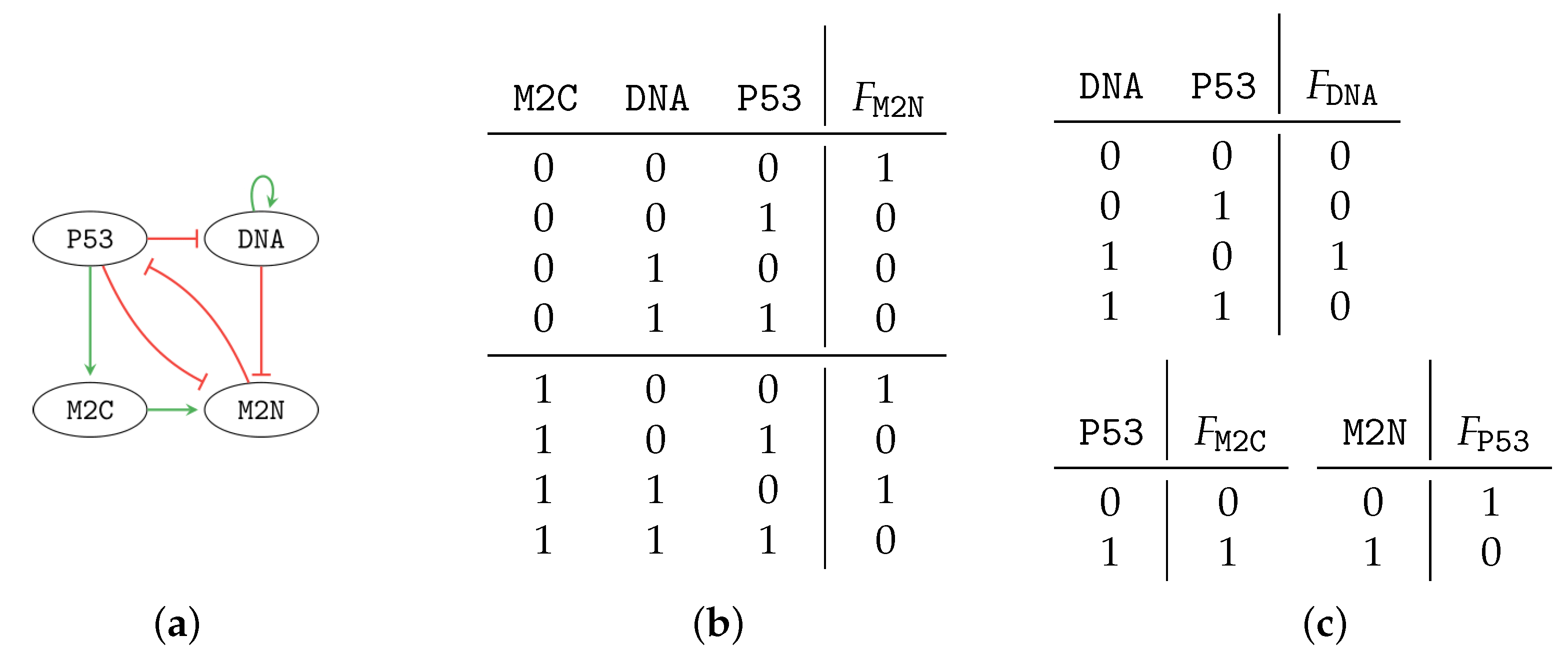
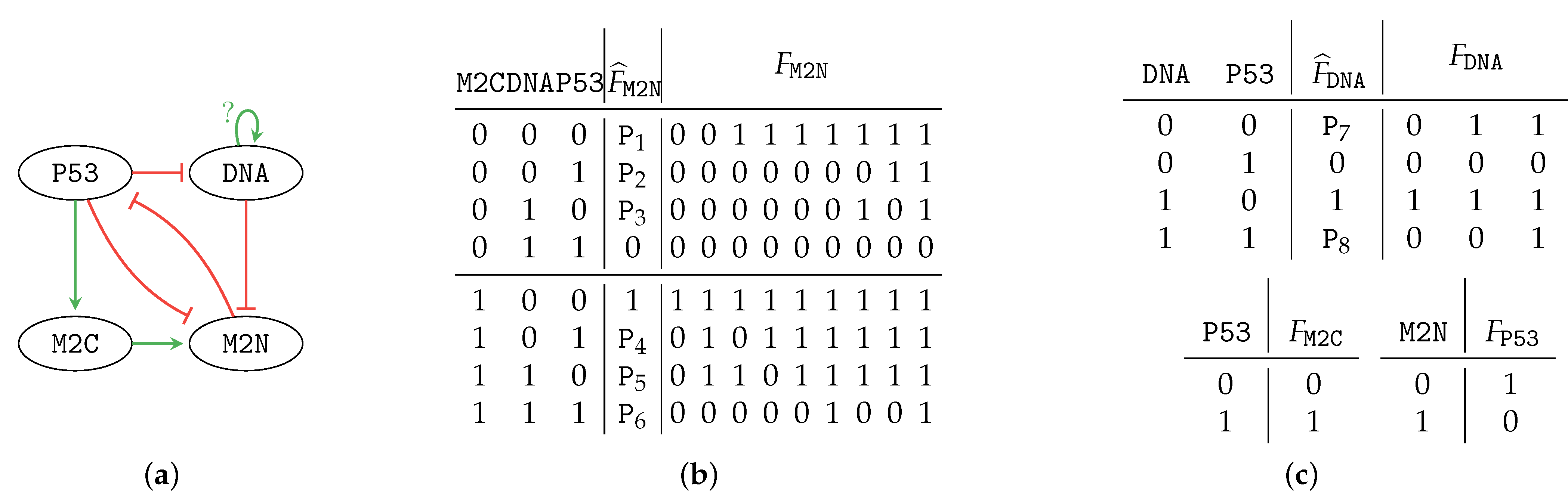
update functions which specify the way variables dynamically change their value based on influences from other variables. Typically, influences among variables are visualised in the form of a so-called regulatory network displaying the structure of a BN (an example is shown in
Figure 1a).
In BN models, time is considered to be
discrete. At each time step, some variables are selected for an update. The scheduling of updates has a strong influence on the reachable configurations of the variables. There are two dominant updating paradigms. The
synchronous paradigm updates all variables simultaneously, and thus generates deterministic dynamics. In contrast, the (fully)
asynchronous paradigm updates a single non-deterministically selected variable at each time step. In this work, we consider the asynchronous update schedule as it often captures the behaviour of biological systems more realistically compared to its synchronous paradigm [
3].
At any particular time moment, the tuple of all variables’ values in the BN is called a
state of the network. The
state-transition graph (STG) has as its
nodes the states, and each directed edge represents a possible transition from one state to another one in a single update. The size of the STG grows exponentially with the number of variables, which causes the state-space explosion problem [
4]. Since the BN is a finite-state system, the state of the system will in a long-run evolve into a single state (steady-state) or a set of recurring states (a complex attractor). These steady states or recurring states are collectively called
attractors and correspond with the
terminal strongly connected components (TSCC) in the STG. More on BN attractors can be found in [
5].
A significant shortcoming of BNs, when used for modelling real phenomena, resides in the necessity to fully specify the update functions. In practice, it is often complicated to exactly identify Boolean functions from biological data. However, there is typically good evidence of the fact that a variable regulates another one [
6,
7].
Parametrised Boolean networks (ParBN) [
8,
9] address the possibility to specify BNs without the precise knowledge of some update functions; the unknown part is represented in terms of
logical parameters. In ParBNs, only regulators of a variable need to be specified. This allows capturing multiple variants of the possible actual behaviour of variables without conducting many more expensive experimental observations. A disadvantage of ParBNs is that their analysis is significantly more difficult compared to the non-parametrised case as the edges in the STG change according to the chosen
parametrisations, i.e., a particular setting of logical parameters in the specification of update functions.
The goal of the Boolean network control is to influence the behaviour of the network so that it stabilises in a particular attractor. A typical way to change the behaviour is to perturb the values of some variables. In this paper, we consider one-step state perturbations in which we apply all the perturbations of variables simultaneously and only once. After the perturbation, the system is left to behave normally. Solutions of the BN control problem for a model of a cell in silico provide the basis for experimental designs allowing reprograming the cell in vitro. Since the practical realisation of particular perturbations requires non-trivial effort, the number of perturbations typically needs to be minimised. To that end, the control problem is usually enriched with some optimisation criteria.
Typically, two elementary types of control problems are distinguished: (i) achieving a single desired target attractor irrespective of the current state (target control) [
10], (ii) achieving control between every pair of attractors (full control) [
11].
The target control problem has been studied in non-parametrised BNs with both the synchronous and asynchronous update. In synchronous case, the method [
10] identifies the control kernel, a minimal set of nodes, inferred from the explicit STG of the BN. In [
12] a network graph aggregation approach is employed at the level of the regulatory network avoiding construction of the full STG. In [
13], the regulatory network is divided into partially dependent parts identified as strongly connected components. In the case of asynchronous BNs, the approach in [
14] computes a set of relevant BN variables based on the identification of particular motifs in the regulatory network.
Traditional approaches mentioned above assume the control to be implemented by involving a permanent perturbation applied continuously for an extended period of time. However, this is not possible to be efficiently achieved in practise [
15]. To that end, the concept of one-step perturbation has been introduced in [
16] in the context of asynchronous BNs (the perturbation is applied in the initial state, and after that, the system evolves according to its original dynamics). The algorithms in [
16] address both target and full control, and they solve the existential problem as well as the optimal problem (identifying the minimal set of perturbations). The method is based on an efficient identification of a strong basin. In this paper, we employ a similar idea for the target control in the novel context of ParBNs.
It is also worth noting that in [
17,
18] the authors work with the concept of temporary perturbations filling the gap between one-step and permanent perturbations. Moreover, complex control strategies considering temporal sequences of perturbations are studied in [
19,
20,
21,
22]. All those results are developed for non-parametrised BNs only.
All listed existing methods for BN control are difficult to lift on ParBNs. That is because the naïve solution considering iteration of a method for every parametrisation would suffer by the combinatorial explosion of the parameter space.
In this paper, we focus on the
source-target variant of the ParBN control problem. To the best of our knowledge, we provide the first efficient solution to this problem. It is worth noting that the parameters bring many new challenges to the control problem. First, the attractors might significantly differ with the change in the parametrisation of the network. Second, the minimal state perturbation does not necessarily work for all parametrisations, and therefore, the notion of the optimal control strategy needs to be adapted to such a situation. Third, the parameter-space explosion (in addition to the state-space explosion) makes the problem computationally demanding. The parameter space is in the worst case, doubly exponential [
23]. Each ParBN parametrisation generates a unique BN model with a unique STG. That is why using algorithms developed for asynchronous non-parametrised BNs and computing the control set for each parametrisation distinctly (parameter scan) is not feasible, and a new approach needs to be developed.
We propose an efficient alternative to the naïve parameter scan approach to compute the one-step target control of ParBNs. Technically, our approach relies on the integration of several formal methods. In particular, we employ a representation of ParBNs based on a symbolic edge-coloured graph using BDDs [
9,
24]. For this representation, we extend a well-established algorithm for asynchronous BNs control employing one-step perturbations [
16]. The technique is based on the identification of attractor’s strong basin (states from which it is possible to reach only the attractor). Our novel algorithm is able to compute the strong basins of all ParBN parametrisations simultaneously instead of computing them one by one (individually for every parametrisation). We show that for highly parametrised models, our approach is significantly more efficient than the naïve approach.
3. Control Problem for Parametrised Boolean Networks
A computational model is controllable if we can assure that from some initial state, it reaches a desired final state in a finite amount of steps. This property was well-studied in the context of synchronous BNs [
10,
28] and is also being pioneered for asynchronous BNs [
18,
29]. However, the control problem for ParBNs has not been explored yet. ParBNs offer a more flexible representation of biological systems by allowing some uncertainty in the specification of the logic behind regulations. Since in reality information on regulatory mechanisms is typically ambiguous or unknown, studying the control problem for ParBNs enables new attractive, real-life applications, such as the discovery of candidate transcription factors for cell reprogramming (i.e., to change a cell’s phenotype) when the model is not fully known.
3.1. Control Problem for Boolean Networks
There are multiple ways to control the behaviour of a BN, mainly differentiated between
state and
function perturbations [
30]. State perturbations force the system to change its current state. Alternatively, function perturbations adjust the update function(s) and therefore modify the edges of the system’s state-transition graph. Typically, changing the processes in a cell (function perturbation) is more difficult than artificially adding or extracting a biochemical substance (state perturbation). For this reason, this paper focuses on state perturbations.
State perturbations can be further differentiated based on their temporal characteristics, mainly one-step, sequential, temporary, and permanent control. In one-step control, we change the values of the controlled variables once, and then the network evolves as originally defined. Sequential control identifies a sequence of perturbations that are applied at different time steps. When applying the control temporarily, there exists a finite amount of computational steps after which the control is released. Finally, the most intrusive control is permanent control of variables. However, this scenario is rather unrealistic in practice, as the given substance would need to be added or extracted forever. Moreover, the permanent perturbation might disrupt the original long-term behaviour of the network or introduce completely new behaviours.
Finally, we consider different control objectives, defined in [
16] as follows:
- (i)
Source-target control: Given a source state, and a target attractor, find such control that when applied, the BN always converges from the state s to the attractor T.
- (ii)
Target control: Given a target attractor, find a control for every source attractor (such that ) that when applied, the BN converges from S to T.
- (iii)
Full control: For all pairs of distinct attractors , find a control which guarantees that the BN converges from S to T.
- (iv)
All-pairs control: Given a subset of source attractors and target attractors , for every pair and , find a control which guarantees that the BN converges from S to T.
In some cases, one may also choose when the control is applied. Here, we consider
immediate control, i.e., the control applied to the given state. Alternatively, during
sequential control, the perturbations can be applied multiple times at different time points. This way, we can sometimes control the system using fewer perturbations. However, this approach brings new issues, such as dealing with the non-determinism of the BN (different perturbations may be necessary in different branches of the non-deterministic network’s behaviour). Moreover, we would need to be able to precisely observe a current state of the BN. These issues can be addressed to some extent using
attractor-based sequential approach [
20].
In summary, the control problems for BNs differ in the following aspects:
What do we want to control; goal: What is the initial state of the BN? Where we want to end? Do we want to control only one scenario or multiple scenarios?
What control we apply: We can either perturb states (once, temporarily, forever) or functions of variables;
When we apply control: Only once from an initial state in contrast with applying control to an arbitrary state and any amount of times.
3.2. One-Step Control Set of Parametrised Boolean Networks
In this paper, we focus on state perturbations applied immediately in the initial state. This is the elementary way to perturb the system when solving the source-target control problem. The respective notion of one-step control is stated formally in the following definition.
Definition 7 (One-step control of ParBN)
. Given a ParBN , a one-step state perturbation control
C (further referred simply as control
) is a tuple where , and are mutually disjoint (possibly empty) subsets of variables of . The set of all possible controls is denoted . An application of control
C to a state s, denoted , results in a state defined as:The size of C is defined as .
Next, we focus on establishing the control problem (when computing the one-step perturbation control) in ParBNs. Conceptually, the parametrised control problem is to some extent similar to the parameter synthesis problem. The goal of parameter synthesis is to find parametrisations that ensure some desired behaviour in the network. Such behaviour can also involve reachability of specific attractors. However, the critical distinction between parameter synthesis problem and control problem is that in control, one determines perturbations that lead to a particular objective (with respect to given parametrisations), possibly resulting in behaviour that is not achievable only by tuning the network parameters. In this work, we thus treat parameters as unknown properties of the system rather than components that can be influenced.
One of the most significant challenges of ParBN control is that the attractors change based on the parametrisation. To that end, it makes sense to solve the control problem only for parametrisations which admit the given attractor. The parametrised control problem then computes a mapping that associates a potential control with the maximal set of parametrisations for which the control is applicable (the so-called control enabling parametrisations). Formally, the considered parametrised control problem is stated in the following definition.
Definition 8 (Source-target control in ParBN). Given a ParBN , a source state s and a target state t, find a mapping which assigns each control a maximal (possibly empty) set of parametrisations p for which when C is applied, converges from s to . We refer to as the control enabling parametrisations for C.
Intuitively, control enabling parametrisations are the parametrisations, for which the target state is achieved by applying C in the non-parametrised case. Please note that source-target problem in the context of ParBN is aiming to drive the network into a target state of some attractor instead of an attractor itself. This is because parameterisations might contain attractors which are considered similar to all of them contain the given state. Therefore, in all parameterisations the given state t is entered infinitely often by the controlled BN. If this is not the case of some ParBN and some parametrisations contain attractors which are out of the interest, the set of parameterisations might be replaced with an arbitrary one.
It is worth noting that it is always possible to bring the system into the given target state by setting the ParBN’s variables to the values adequately (with the values of the given target state). We call this control trivial. However, when controlling a system, we typically look for a control which requires the fewest interventions possible. Therefore, we want to minimise the number of the controlled variables and the trivial solution might not be optimal. In a non-parametrised setting, this is typically the only considered optimisation criterion.
In a ParBN, the situation is further complicated due to the dependence on the parameters. To reach some attractor, it is sufficient to reach its strong basin after the application of a control. Nonetheless, the strong basin of an attractor can vary according to the parametrisation, and the control thus “works” only for control enabling parametrisations. We are interested maximising the number of this type of parametrisations. To capture this property of ParBN control we introduce the notion of robustness that normalises the number of control enabling parametrisations:
Definition 9 (Robustness of control)
. Given a ParBN , a target state t, a control set C and , the robustness of control
C is defined as the ratio between the number of control enabling parametrisations and the number of all relevant parametrisations: Unfortunately, it is not always possible to ensure that some control is both minimal and the most robust. For example, there may be a control set
C small in size, which only works for a small fraction of the parameter space. Consequently, while
C is easily applicable, it may be unlikely to work in reality, as the real behaviour of the system can also follow one of the parametrisations which are not controlled by
C. We discuss this issue in more detail in
Section 5.
4. Materials and Methods
We are now ready to describe our computational framework for solving the one-step state perturbation control of ParBN. We start by introducing our approach for finding strong basins in a ParBN. Then we explain the framework for exploring ParBN’s STG and for manipulation with ParBN’s parametrisations. Finally, we build a concise workflow for ParBN control employing the proposed algorithms.
4.1. Semi-Symbolic Parametrised Strong Basin Search Algorithm
We assume the set of parametrisations of a ParBN is represented as a reduced ordered binary decision diagram (BDD) [
24]. The decision variables of the BDD are the parameters of the network (
), meaning that every path from the root to a leaf in such a BDD represents a parametrisation of the ParBN. Common logical operations on such BDDs (and, or, negation, …) then correspond to set operations (intersection, union, complement, …). Furthermore, static constraints (activation, inhibition, observability) can be formalised using Boolean formulae over
, and we can, therefore, create a BDD which enforces all imposed constraints and represents the set of all valid parametrisations.
Recall that we represent as an edge-labelled state-transition graph, where each transition has an associated set of parametrisations represented as a BDD. A parametrised state set is a mapping assigning to each state a set of parametrisations. Furthermore, we suppose that the state space is represented explicitly, meaning that all operations on states are performed element-wise (typically in parallel).
We consider parametrised reachability procedures — given a source state
s and a parameter set
P, these procedures compute a maximal parametrised state set of all forward/backward reachable states from the source state
s (containing all reachable states
t where each
t is associated with a maximal set of parametrisations
for which
t is reachable from
s):
The chosen representation (explicit state space and symbolic parametrisations) allows computing the reachability procedures in parallel. For the underlying implementation, we are working with internal libraries of the tool Aeon [
31] which provides most of the necessary functionality, including a convenient format for specifying ParBNs and parallel reachability procedures.
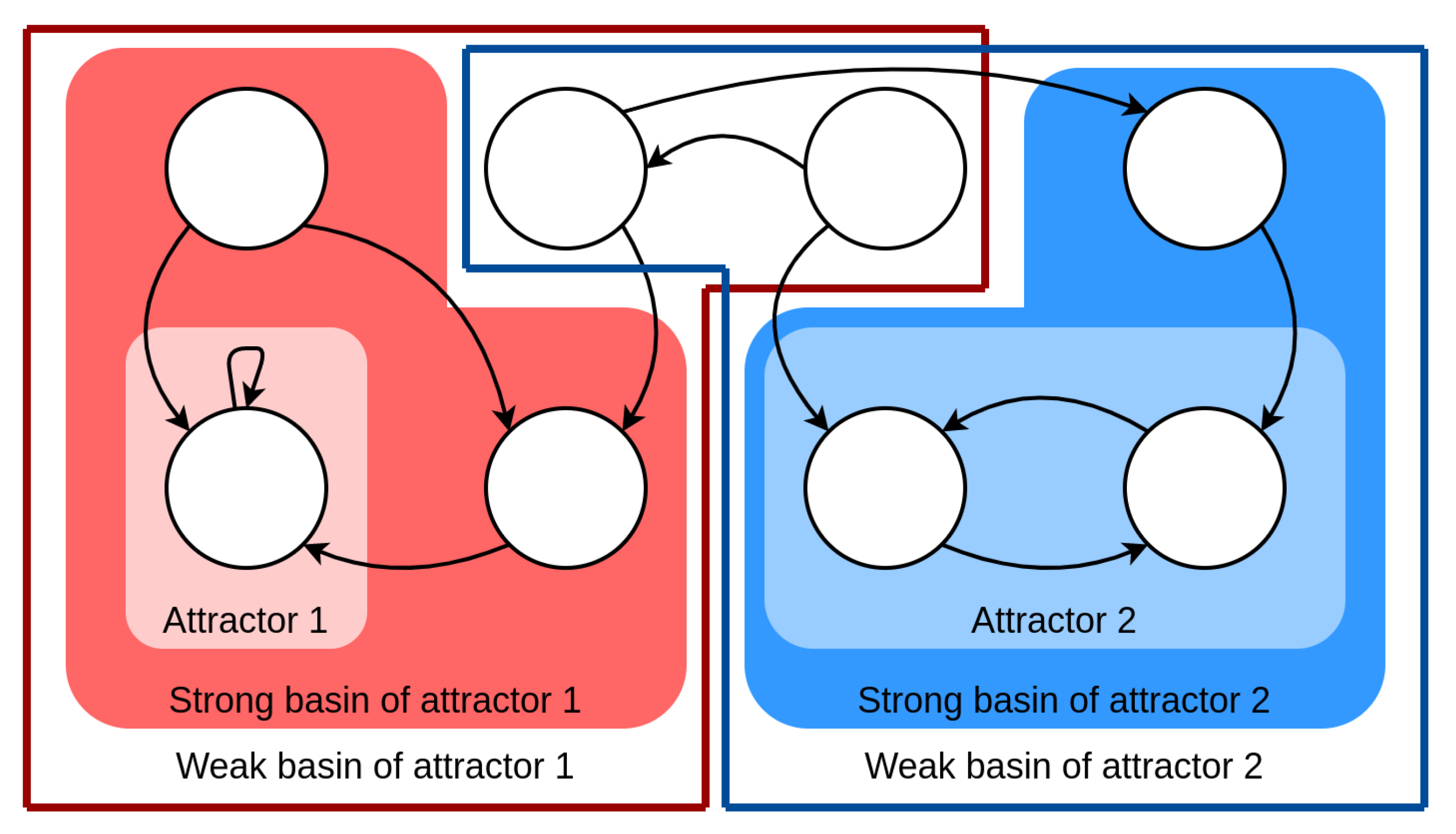
The key observation for controlling ParBNs is that an attractor is always reached from its strong basin (see Definition 4). From all other states, it is possible to reach also some other attractor(s); therefore, reaching the target attractor is not guaranteed. When the attractor’s strong basin for all parametrisations is known, we can compute the control mapping from a source state to the target attractor by considering Hamming differences between the source and the states of the strong basin.
Our algorithm is based on the fixed-point approach for strong basin computation in non-parametrised BNs [
32]. The premise is that only states from which it is possible to reach the attractor (weak basin) can be part of the strong basin. The weak basin of the attractor is computed using some standard reachability algorithms, for example, BFS. Then states are iteratively removed if it is possible to leave the basin from them (and therefore not reach the given attractor). Finally, if there are no states left to remove, the fixed-point is achieved, and the strong basin is found.
For parametrised control, we first need to determine for the target state t, since in all other parametrisations, t is not a part of any attractor. This process is described in Algorithm 1. The algorithm is following: we first compute all reachable states, but only the one from which we can also reach back the target state itself are a part of a TSCC. Otherwise, it is possible to reach some other component of the system from the target state, and that contradicts the notion of attractor. In the parametrised setting, we obtain a mapping of states to parameterisations in which it is not possible to return to the target again. Therefore, in all these parametrisation the target state is not a part of any attractor, and so we discard them from the full parameter space P to obtain .
In Algorithm 2, we extend the approach from [
32] onto ParBN. For each state we remember under which parametrisations it is in the basin, starting with the parametrised weak basin. Then we iterate over the basin’s states. For each state, we consider its successors, and we compute the parametrisations for which some successor is
not in the strong basin. In these parametrisations, it is possible to leave the basin, and therefore these parametrisations are not part of the strong basin, and so we remove them for this state. We can process the states in parallel and compute for them the parameterisations which are not part of the strong basin. To avoid writing to the strong basin structure while it is intensively read from, we store the parameterisation which should be removed separately, and after it is computed, we update the strong basin structure sequentially. The procedure is repeated until nothing more can be removed from the strong basin.
| Algorithm 1: Compute attractor parametrisations . |
Input: PBN , target attractor state
Output: Attractor parametrisations
;
;
/* For every state, compute the BDD difference */
;
return;
|
| Algorithm 2: Compute strong basin for an attractor in parallel. |
![Mathematics 09 00560 i001]() |
4.2. Control Computation Workflow
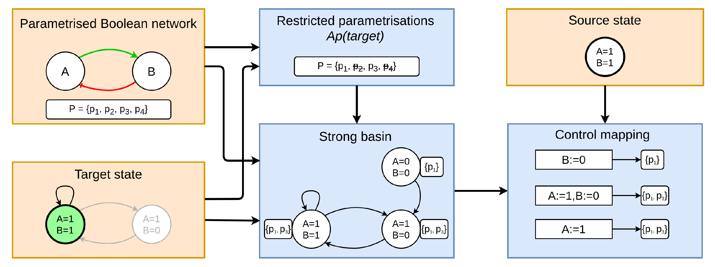
Now we can describe a complete workflow for computing the source-target control in ParBNs, depicted in
Figure 5. The workflow consists of three inputs and three computation steps, resulting in the control mapping
.
Given an input ParBN and a target attractor state , we start by computing valid parametrisations set using Algorithm 1. Then, the parametrised strong basin is computed from the ParBN with target attractor state and its valid parametrisations using Algorithm 2. After that, from the strong basin and the source state, we obtain the complete control mapping. Notice that we do not need to know the source state for computing the strong basin and that we can re-use the target’s strong basin for obtaining control for different sources.
To compute the control mapping, observe that viable controls correspond exactly to the Hamming differences (the variables with opposite values) between the source state and the states of the strong basin; yielding one viable control C for every state s in the strong basin . Any other control does not reach the strong basin and therefore does not guarantee to reach the target attractor (for these, ). A control C is then viable only for parametrisations for which s appears in the strong basin, we thus set .
Finally, we can compute the size and robustness of each control as we have all knowledge regarding the variables which need to be controlled and parametrisations for which the controls work. If it is desired, we can construct a witness BN for a control C (a non-parametrised BN where the given control works) by fixing some parameter from .
In highly parametrised models, it is not unusual to obtain a control with size 0, where in some parametrisations no action would be needed to control the model. This is because, in some parametrisations, the source might already be a part of the target’s strong basin. If this case is considered unrealistic (since there is probably a need for control, thus these parametrisations appear to be invalid), the parametrisations can be replaced with a custom set of parametrisations.
The resulting set of all available controls can be then used for e.g., cell reprogramming. However, we might obtain many possible controls, and we need to decide which one should be applied. To do that, we can decide based on the size of control or its robustness. The control set can be arbitrarily filtered discarding controls with size bigger than the trivial control (which always has 100% robustness) or bigger than some set size. Similarly, the control set can be pruned based on too low robustness. It is left to the actual application to decide which control would best suit its needs. Namely, whether it is more important for the control set to be small or to be robust, as typically, there is rarely available control which would be optimal in both these factors.
5. Results
We evaluate our approach on two real-life BN models. We compare the performance of our approach using a different number of parameters implanted into the models, resulting in different size of relevant parameter space. We conducted all measurements using a machine equipped with AMD Ryzen Threadripper 2990 WX 32-Core Processor and 64 GB of memory.
The first model is a
cell-fate decision model [
33]. The model provides a high-level view of possible different cell fates such as pro-survival, necrosis or apoptosis. We used a fully parametrised version (all update functions are completely parametrised) of this model, and we selected seven biologically relevant attractors. We computed strong basins only for these attractors in several parametrised versions of the model differing in the number of unknown parameters (see
Table 1).
The second model, a
myeloid differentiation network [
34], was designed to model a bone marrow tissue cell differentiation from common myeloid cell to specialised blood cells (megakaryocytes, erythrocytes, granulocytes, and monocytes). The original non-parametrised network has eleven nodes and six attractors. We derived several parametrised versions of the model by arbitrarily parametrising update functions of the model. Similarly to the previous case, we used only attractors of the original network when computing strong basins for parametrised versions of the model. The results are again shown in
Table 1.
Next, we “virtually” compare our approach to the naïve parameter-scan approach. In [
16], a strong basin of (non-parametrised) asynchronous BNs is computed using a block decomposition method with 4 ms needed to finish the computation for the
myeloid model. Even if the reported hardware was slower than in our case and we assume that the strong basin computation for one parametrisation would last only 1 ms, the fully parametrised myeloid model contains an attractor which is present in 3.7 × 10
9 parametrisations. Therefore, the expected time for computing a strong basin for all parametrisations with 32-fold parameterisation is more than a day compared to less than 27 s achieved using our parameter-based semi-symbolic approach.
We evaluate the scalability of our approach on a fully parametrised myeloid model. The results are shown in
Table 2. The computation was restricted to the specified amount of CPUs. The final speed-up achieved on our machine, when using 32 CPUs compared to a non-parallel CPU usage was about 10-fold.
Now let us have a look at an example of how the results might be interpreted and a suitable control selected. Suppose that we want to reprogram an erythrocyte cell (phenotype having factors EKLF = 1 and GATA-2 = 0) into a monocyte cell (phenotype having factors cJun = 1 and EgrNab = 1) of the myeloid model. First, we obtain a strong basin of the monocyte attractor having 1472 states yielding us 1472 possible control sets. We can observe that trivial, i.e., the most robust control strategy (setting variables so that we reach the attractor right after applying the control), has size 8. We can discard all controls with size 8 and larger as they are less optimal in all aspects than the trivial control. In our case, there are 1259 controls with a smaller size than the trivial one.
Resulting smallest control sets have the size 1. However, the best robustness among these controls is 46%. Therefore, it is quite likely that it will not work in practice. If we allow the control to have size 2, we can use the control with 76.8% robustness. Further increasing the size provides control with the size 3 and the robustness 92% and so is highly likely to reprogram the cell’s phenotype. To achieve only slightly more robustness (93.8%), we may use a control of size 5. In this highly parametrised model, there is no control with 100% robustness being smaller than the trivial one. It is not a rule of the thumb that with bigger size of control we obtain better robustness, for example, the control with the size 11 (the only one, with all variables, reversed compared to the original one) has the robustness of only 50%.
It can be seen that the unknown properties of ParBN make selection of one particular “best“ control complicated. The smallest control has low chance to work in reality and while control of size 3 works has significantly better chance to work, the success of the control is not guaranteed, i.e., this is why a careful in vitro experimentation is needed to verify the correctness of the control in reality. Nonetheless, the obtained control set still can help and highly reduce the exponential number of potential transcription factor combinations.


 ,
,  ,
,  ,
,  }. Here,

