A Numerical Comparison of the Sensitivity of the Geometric Mean Method, Eigenvalue Method, and Best–Worst Method

Abstract

In this paper, we compare three methods for deriving a priority vector in the theoretical framework of pairwise comparisons—the Geometric Mean Method (GMM), Eigenvalue Method (EVM) and Best–Worst Method (BWM)—with respect to two features: sensitivity and order violation. As the research method, we apply One-Factor-At-a-Time (OFAT) sensitivity analysis via Monte Carlo simulations; the number of compared objects ranges from 3 to 8, and the comparison scale coincides with Saaty’s fundamental scale from 1 to 9 with reciprocals. Our findings suggest that the BWM is, on average, significantly more sensitive statistically (and thus less robust) and more susceptible to order violation than the GMM and EVM for every examined matrix (vector) size, even after adjustment for the different numbers of pairwise comparisons required by each method. On the other hand, differences in sensitivity and order violation between the GMM and EMM were found to be mostly statistically insignificant.

1. Introduction

Pairwise comparisons constitute a fundamental part of sophisticated multiple-criteria decision-making frameworks, such as the analytic hierarchy/network process (AHP/ANP), PROMETHEE, ELECTRE, PAPRIKA, and many others [1,2,3,4,5,6,7,8,9]. In addition, hundreds of successful applications of pairwise comparisons in almost all domains of human activity have been published in the literature [10].

The objective of a pairwise comparison method is to assign weights to compared objects corresponding to their preference/importance and to rank objects from the most preferred/important to the last. The Geometric Mean Method (GMM) proposed by Crawford [11] and the Eigenvalue (eigenvector) Method (EVM) proposed by Saaty [7] are the most popular methods for deriving weights from pairwise comparisons arranged in the form of a pairwise comparison (PC) matrix. The Best–Worst Method (BWM) proposed by Jafar Rezaei in 2015 (see Rezaei [12]) is one of the latest contributions to the field of pairwise comparisons. It is based on the pairwise comparisons of all objects (in the original paper, the objects were criteria) with the best object and the worst object (known a priori) only. Therefore, it belongs in the family of pairwise comparison methods with missing elements and/or incomplete pairwise comparison matrices (with additional information). Since its introduction, the BWM has attracted the attention of many researchers and practitioners and has been applied to various problems in areas such as waste management, tourism, sustainability or biochemistry [13,14,15,16,17,18].

The appeal of the BWM lies in its obvious simplicity; however, until now, numerical comparisons of the BWM with other methods, the GMM and EVM (AHP) in particular, have rarely been covered in the literature. The studies of Ajrina et al. [19] and Haseli et al. [20] compared the BWM and the AHP via one and two numerical examples, respectively. The original paper on the BWM [12] provided a comparison of the results of the BWM with the AHP in only one particular example based on an experiment with 46 respondents (university undergraduate students) and 322 PC matrices (and pairs of vectors) of the order $n=4$. The work came to the conclusion that the BWM performs better than the AHP, and the weights derived by the BWM are highly reliable. Other comparison studies of the BWM and AHP/GMM are not known to the authors.

Therefore, the aim of this paper is to bridge this gap and provide a comprehensive numerical comparison of the BWM, EVM (AHP), and GMM with respect to two crucial method properties: sensitivity and the violation of the order of preferences (order violation in short). Sensitivity analysis is a well-established tool for assessing how the input of a model/method affects the output (or vice-versa) and is widely used in natural sciences, in particular in climatology [21,22,23,24]. To assess sensitivity, we apply One-Factor-At-a-Time (OFAT) methodology [25]. The second feature we focus on, order violation, describes how often a unit change in the input leads to a change in the final ranking (ordering) of compared objects, therefore providing useful information on the robustness of rankings. As a research method, we apply Monte Carlo simulations, where pairwise comparisons are selected from Saaty’s fundamental scale from 1 to 9 (with reciprocals) and where the number n of compared objects ranges from 3 to 8, as real-world multiple criteria problems usually do not involve large numbers of criteria. Then, we perform a statistical analysis of the acquired results, enabling a final comparison of all three methods.

This paper is organized as follows: preliminaries on pairwise comparison methods, prioritization, sensitivity, and order violation are provided in Section 2, while Monte Carlo simulations are described in Section 3 followed by a discussion in Section 4. Conclusions close the article.

2. Preliminaries

The input data for the PC method is a PC matrix $C=\left[c_{ij}\right]$, where $c_{ij}\in {\mathbb{R}}_{+}$ and $i,j\in \{1,\dots ,n\}$. The values of $c_{ij}$ and $c_{ji}$ indicate the relative importance (or preference) of the objects i and j.

In the context of the BWM, the compared objects are criteria. The set of n criteria to be compared and ranked is denoted as $F=\{F_1,\dots ,F_n\}$.

Definition 1.

The matrix $C=\left[c_{ij}\right]$ is said to be reciprocal if $\forall i,j\in \{1,\dots ,n\}:c_{ij}=c_{ji}^{-1}$ and $C=\left[c_{ij}\right]$ is said to be consistent if $\forall i,j,k\in \{1,\dots ,n\}:c_{ij}·c_{jk}·c_{ki}=1$.

Note that if $C=\left[c_{ij}\right]$ is consistent, then it is also reciprocal, but not vice versa. In this paper, it is assumed that a PC matrix is always reciprocal. The reciprocity condition seems to be natural in many decision-making situations. For instance, if an element $c_{ij}$ of a PCM $C=\left[c_{ij}\right]$ expresses that the i-th criterion is $c_{ij}$ times more important than the j-th criterion, then it is evident that the j-th criterion is $1/c_{ij}$ times more important than the i-th one; thus, $c_{ij}=1/c_{ji}$. In particular, for each criterion i, we obtain $c_{ii}=1$, which corresponds to the fact that the importance of each criterion with respect to itself is equal to one.

2.1. The Eigenvalue Method and the Geometric Mean Method

The result of a pairwise comparison method is a priority vector (vector of weights) w.

According to one of the most popular prioritization methods, the EVM (the Eigenvalue Method) proposed by Saaty [7], the vector w is determined as the rescaled principal eigenvector of the matrix C. Thus, assuming that $C\overline{w}={\lambda }_{\max }\overline{w}$, the priority vector w is $w={[w\left(F_1\right),\dots ,w\left(F_n\right)]}^{\mathrm{T}}=\gamma {[{\overline{w}}_1,\dots ,{\overline{w}}_n]}^{\mathrm{T}}$, where $\gamma$ is a scaling factor, $\gamma ={\left[{\sum }_{i=1}^n{\overline{w}}_i\right]}^{-1}$, so that $\parallel w\parallel =1$.

In the Geometric Mean Method (GMM) (see Crawford [11]) the weight of the $i^{\mathrm{th}}$ alternative is given by the geometric mean of the $i^{\mathrm{th}}$ row of the matrix $C=\left[c_{ij}\right]$. Thus, the priority vector is given as follows:

$$\begin{gathered} {\displaystyle \phantom{(}w={\left[w\left(F_1\right),\dots ,w\left(F_n\right)\right]}^{\mathrm{T}} \\ =\gamma {\left[{\left(\prod _{r=1}^n{c}_{1r}\right)}^{\frac{1}{n}},\dots ,{\left(\prod _{r=1}^n{c}_{nr}\right)}^{\frac{1}{n}}\right]}^{\mathrm{T}}} \end{gathered}$$

(1)

where $\gamma ={\left[{\sum }_{i=1}^n{\prod }_{r=1}^n{c}_{ir}\right]}^{-1}$ is the scaling factor again.

Several aspects of these methods are discussed in more detail, e.g., in Ramík [26].

2.2. The Best–Worst Method

In the Best–Worst method (see Rezaei [12]), each criterion is pairwise compared only with the best criterion and the worst criterion.

The Best–Worst method proceeds as follows [12]:

Step 1.

A set of criteria is determined.

Step 2.

 The decision maker identifies the best (most desirable, most important) criterion and the worst (least desirable, least important) criterion.

Step 3.

 Preferences of the best criterion with respect to all other criteria are determined on a scale from 1 (equal importance) to 9 (absolute preference).

Step 4.

 Preferences of all other criteria with respect to the worst criterion are determined onathe scale from 1 to 9.

Step 5.

 Optimal weights of all criteria are found by solving a corresponding non-linear programming problem; see Equation (2).

Let $c_{Bj}$ denote the preference of the best criterion (B) over the criterion $F_j$, and let $c_{iW}$ denote the preference of the criterion $F_i$ over the worst criterion (W). Let $w_B$ and $w_W$ be the weights of the best and worst criterion, respectively. The goal is to find the vector of criteria weights (a priority vector) $w=(w_1,w_2,\dots ,w_n)$.

Rezaei [12] suggested finding the priority vector by solving the following optimization problem:

$$min\left(\underset{j}{max}\left\{\left|\frac{w_B}{w_j}-c_{Bj}\right|,\left|\frac{w_j}{w_W}-c_{jW}\right|\right\}\right)$$

(2)

s.t.

$$\sum _{j=1}^n{w}_j=1$$

(3)

$$w_j\ge 0,\forall j=1,\dots ,n.$$

(4)

The problem can equivalently be stated as follows:

$$min\xi$$

(5)

s.t.

$$\left|\frac{w_B}{w_j}-c_{Bj}\right|\le \xi ,\forall j=1,\dots ,n,$$

(6)

$$\left|\frac{w_j}{w_W}-c_{jW}\right|\le \xi ,\forall j=1,\dots ,n,$$

(7)

$$\sum _{j=1}^n{w}_j=1,$$

(8)

$$w_j\ge 0,\forall j=1,\dots ,n.$$

(9)

Further, it is assumed that for all j, the following inequalities hold:

$$c_{BW}\ge c_{jW}\ge 1;c_{BW}\ge c_{Bj}\ge 1.$$

(10)

A linear version of the BWM was introduced by Brunelli Rezaei [27] and Rezaei [28], where the letter “$\mathit{L}$” denotes linear:

$$min{\xi }_{\mathit{L}}$$

(11)

s.t.

$$\left|w_B-c_{Bj}{w}_j\right|\le {\xi }_{\mathit{L}},\forall j=1,\dots ,n,$$

(12)

$$\left|w_j-c_{jW}{w}_W\right|\le {\xi }_{\mathit{L}},\forall j=1,\dots ,n,$$

(13)

$$\sum _{j=1}^n{w}_j=1,$$

(14)

$$w_j\ge 0,\forall j=1,\dots ,n.$$

(15)

Notice that the solution to the linear version of the BWM differs from the solution to the non-linear version in general. In addition, in this case, the value of ${\xi }_{\mathit{L}}^{*}$ should not be divided by $\mathit{CI}$.

When comparing n objects (criteria, alternatives, etc.) pairwise, the EVM and GMM require $n(n-1)/2$ comparisons to be made. The BWM requires only comparisons (of criteria) with the best and worst criterion, and the reduced number of comparisons amounts to $2n-3$. This reduction might be very important when dealing with a large number of compared objects.

2.3. Order Violation

First, let us explain the concept of order violation.

Definition 2.

Let $C=\left[c_{ij}\right]$ be a pairwise comparison matrix of n objects, let $c_{ij}\in \left\{\frac{1}{9},\frac{1}{8},\dots ,1,\dots ,8,9\right\}$, and let $w=(w_1,\dots ,w_n)$ be a corresponding vector of weights (a priority vector). The order violation occurs when for some pair of objects $(i,j)$, $i,j\in \{1,\dots ,n\}$, with the weights $w_i$ and $w_j$, respectively, it holds that after a change of one element $c_{kl}$, $k,l\in \{1,\dots ,n\}$, by one unit of the scale, the relation $w_i\ge w_j$ changes into $w_i<w_j$.

 

Remark 1.

By a unit change in Definition 2, we mean the change to an adjacent point of a given discrete scale; e.g., a change from 6 to 7 (and reciprocal values change as well), or from $\frac{1}{6}$ to $\frac{1}{7}$ (and reciprocal values also change again). In addition, other scales than Saaty’s fundamental scale can be used for comparisons, but we decided to adhere to the scale of the original study of Rezaei [12].

Order violation means that after a change of only one pairwise comparison by just one unit (which is a minimal possible change) the order (ranking) of compared objects provided by the given PC method changes as well. Thus, it can be considered an undesirable feature, as it indicates that the order of objects is unstable and a minimal change or error is sufficient to disturb it.

2.4. Sensitivity

To evaluate the sensitivity of the BW, EV, and GM methods, we applied One-Factor-At-a-Time (OFAT) methodology. We define sensitivity as a change in the priority vector (output) when one preference (input) is changed by one unit:

Definition 3.

Let $w=(w_1,\dots ,w_n)$ be the vector of weights obtained by a generic prioritization method $\mathit{PM}$. Let $w^{*}=(w_1^{*},\dots ,w_n^{*})$ be the vector of weights after one preference was changed by one unit. Then, the sensitivity $△w$ is defined as follows:

$$△w_{\left(n\right)}^{\left(\mathit{PM}\right)}=\frac{100}{n}\sum _{i=1}^n|w_i-w_i^{*}|.$$

(16)

The sensitivity $△w$ expresses, in a percentage, a per-weight change in the original priority vector w. If, for instance, $△w_{\left(n\right)}^{\left(\mathrm{GMM}\right)}=2$, this means that each component of the original weight vector $w=(w_1,...,w_n)$ changed by 2% on average when the GMM was applied.

The following example illustrates the use of order violation and sensitivity.

Example 1

(Best Worst Method [29]). Consider buying a car according to five criteria: quality, price, comfort, safety, and style. The best criterion is price, and the worst criterion is style. The buyer provides the following pairwise comparisons:

Best to all preferences: $(2,1,4,3,8)$. All to worst preferences: $(4,8,4,2,1)$.

By using the linear BWM model and the MS Excel Solver from Best Worst Method [29], we obtain the following weights of criteria:

$$w=(0.246,0.431,0.123,0.154,0.046).$$

Now, we change one preference by one unit (in bold) in the best to all preferences: $(2,1,\mathbf{3},3,8)$. The weights of criteria are now

$$w^{*}=(0.233,0.427,0.155,0.136,0.048).$$

The sensitivity $△w_{\left(5\right)}^{\left(\mathrm{BWM}\right)}istherefore\frac{100}{5}{\sum }_{i=1}^5|w_i-w_i^{*}|=1.4$.

Thus, the weights of the criteria changed, on average, by 1.4%.

As for the order violation, initially the criterion of comfort’was ranked fourth and the criterion of safety was ranked third. After the unit change in one PC comparison, the criterion of comfort was ranked third and the criterion of safety was ranked fourth. Therefore, an order violation occurred.

3. Monte Carlo Simulations

Simulations of the EVM and GMM were performed in C#; simulations of the BWM were carried out via the MS Excel Solver [29].

The procedure for a full PC matrix, the GMM (EVM), and Saaty’s scale was as follows:

Step 1.

 A random PC (reciprocal) matrix C of the order n with entries from Saaty’s scale (from 1 to 9) was generated.

Step 2.

 The priority vector w was derived by the GMM (EVM).

Step 3.

 A randomly chosen element ${}_{c_{ij}}$ of a PC matrix C was randomly changed by one unit of a scale up or down, and the reciprocal element ${}_{c_{ji}}$ was changed accordingly.

Step 4.

The priority vector $w^{*}$ was derived by the GMM (EVM).

Step 5.

 Sensitivity (16) was calculated and order violation was checked.

Step 6.

 The procedure was repeated 500–1000 times for each matrix size $n\in \{3,4,5,6,7,8\}$.

The EVM and GMM were performed on the same set of random PC matrices.

The procedure for the BWM and Saaty’s scale was as follows:

Step 1.

 Pairwise comparisons of all n objects with respect to the best and the worst object (in the form of two vectors) were randomly generated with the use of Saaty’s scale while preserving relations (10).

Step 2.

 The priority vector w was calculated by the linear version of the BWM according to Equation (11).

Step 3.

 A randomly chosen element from one of the two vectors generated in Step 1 was changed by one unit (up or down, again randomly), while preserving Saaty’s scale.

Step 4.

 The priority vector $w^{*}$ was derived by the linear BWM according to Equation (11).

Step 5.

 Sensitivity (16) was calculated and order violation was checked.

Step 6.

 The procedure was repeated 500–1000 times for each matrix size $n\in \{3,4,5,6,7,8\}$

Table 1. Simulation results: mean sensitivity and average order violation occurrence (for each method separately). BWM: Best–Worst Method; GMM: Geometric Mean Method; EVM: Eigenvalue Method.

Method	n	Mean Sensitivity (st. dev.)	Order Violation (%)
BWM	3	02.801 (2.7771)	0
	4	2.161 (2.170)	31.4
	5	1.621 (1.687)	38.9
	6	1.273 (1.276)	50.8
	7	0.966 (1.031)	53.8
	8	0.741 (0.831)	97.2
GMM	3	1.942 (1.475)	10.6
	4	0.919 (0.681)	12.2
	5	0.465 (0.364)	12.3
	6	0.263 (0.212)	15.2
	7	0.185 (0.148)	19.1
	8	0.113 (0.081)	61.0
EVM	3	1.790 (1.444)	10.9
	4	0.932 (0.619)	14.8
	5	0.474 (0.314)	16.6
	6	0.304 (0.178)	22.0
	7	0.196 (0.094)	24.3
	8	0.134 (0.059)	64.7

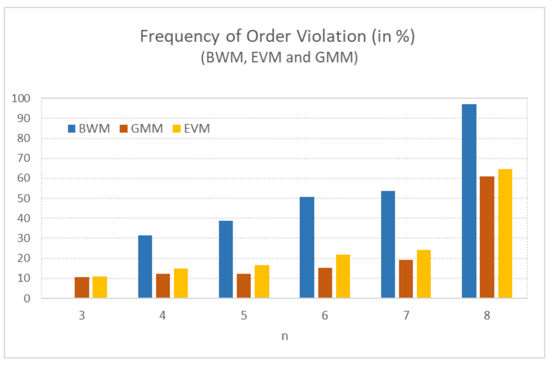
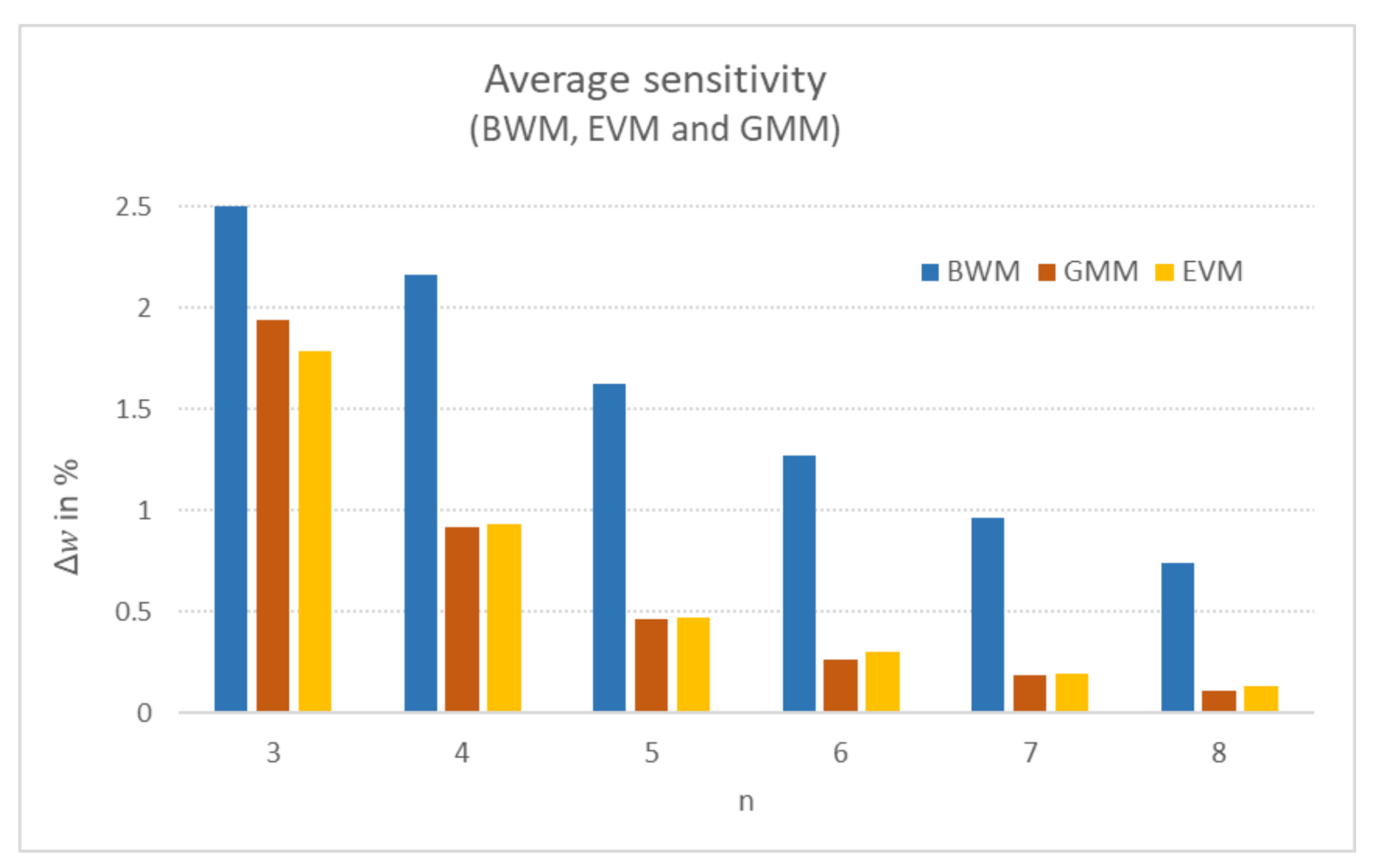
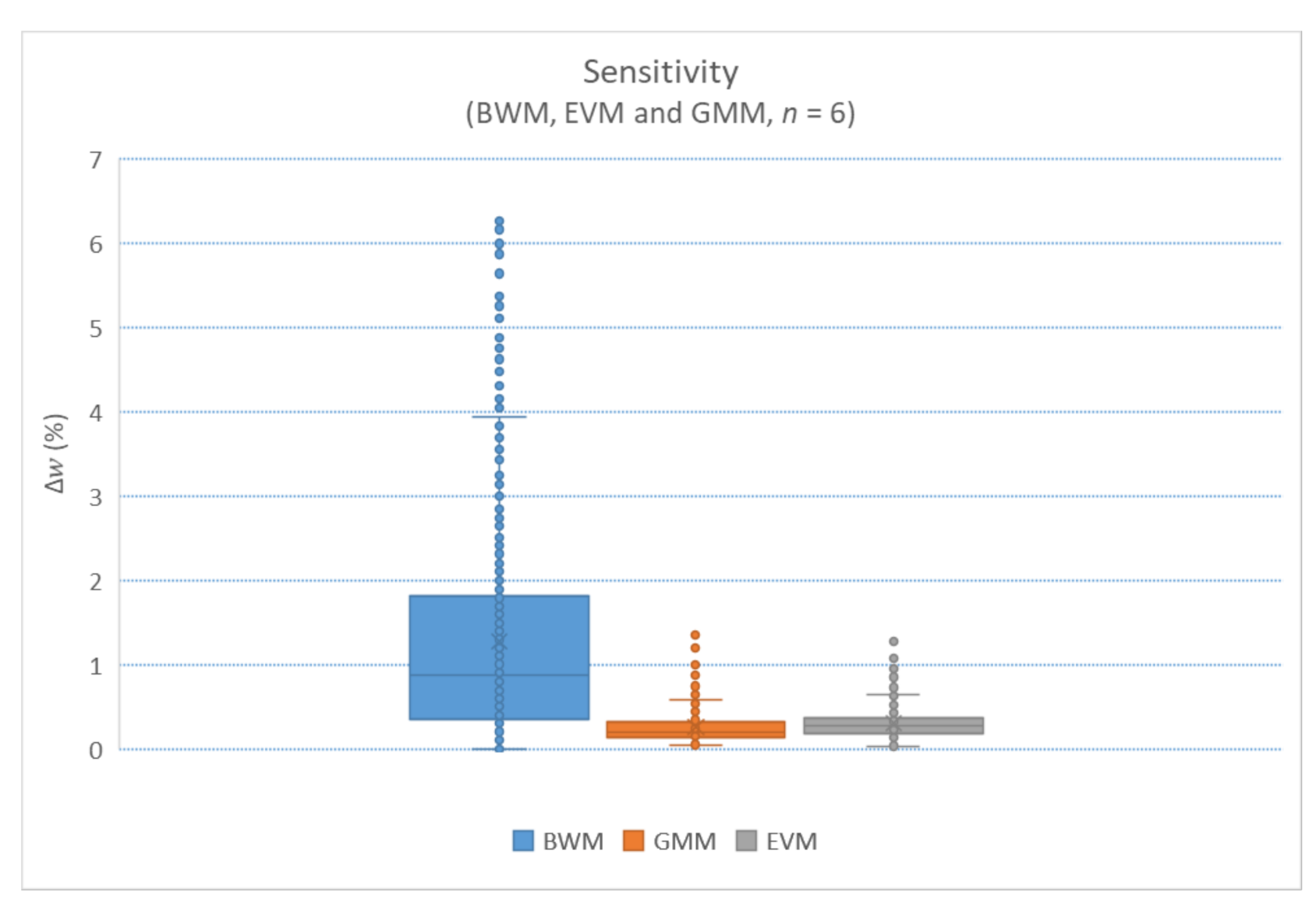
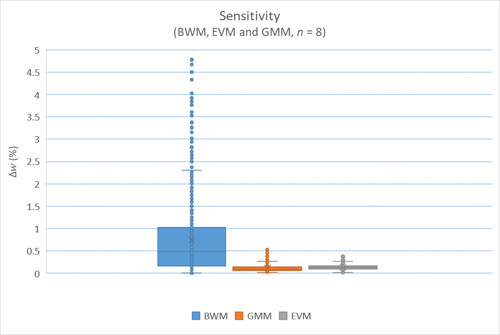
provides the average values of sensitivity along with standard deviations and the frequency of the order violation. As can be seen, the least sensitive (thus, the most robust) method was the GMM followed by the EVM. The Best–Worst method performed significantly worse. In the case of order violation, again, the GMM performed best and the BWM worst.

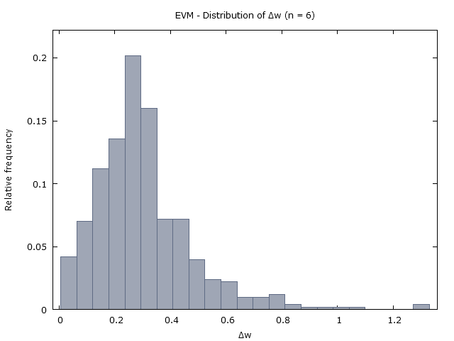
Figure 1 and Figure 2 provide graphical illustrations of the sensitivity and order violation for all examined matrix sizes.

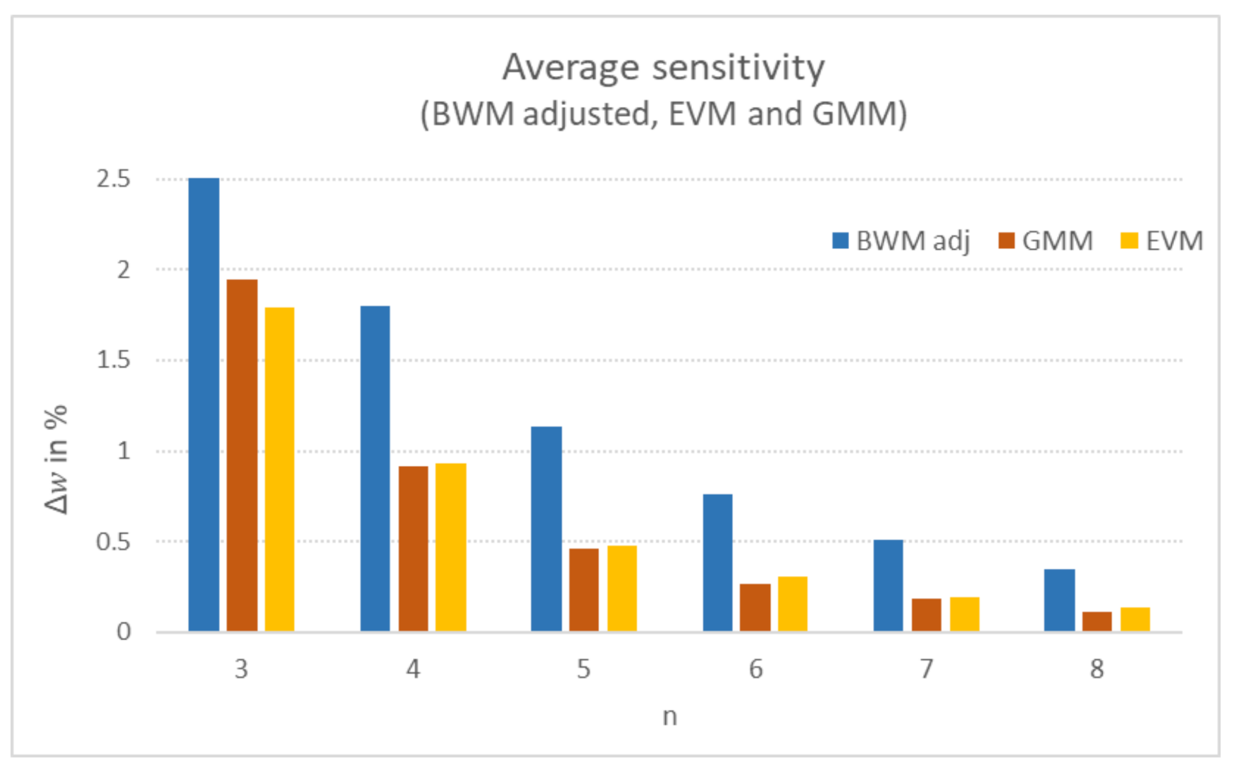
Figure 3 shows a comparison of the GMM and EVM with the BWM adjusted for the lower number of pairwise comparisons.

Figure 4, Figure 5 and Figure 6 show the sensitivity distribution of all three methods for $n\in \{4,6,8\}$.

Figure 7, Figure 8 and Figure 9 provide frequency diagrams of the sensitivity for all three methods and $n=6$.

A discussion of the results is provided in the next section. The data are available in the Mendeley repository [30].

4. Discussion

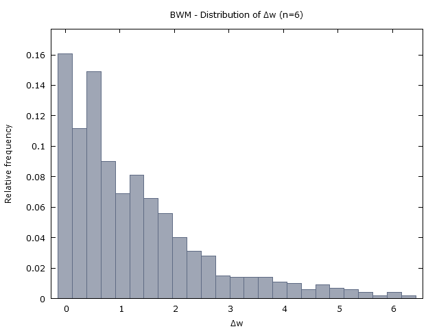
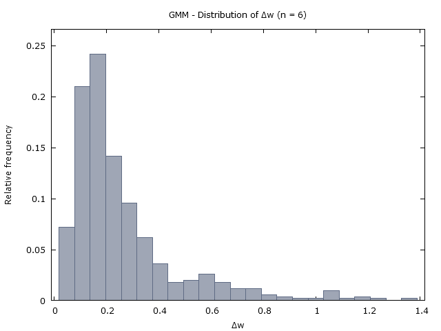
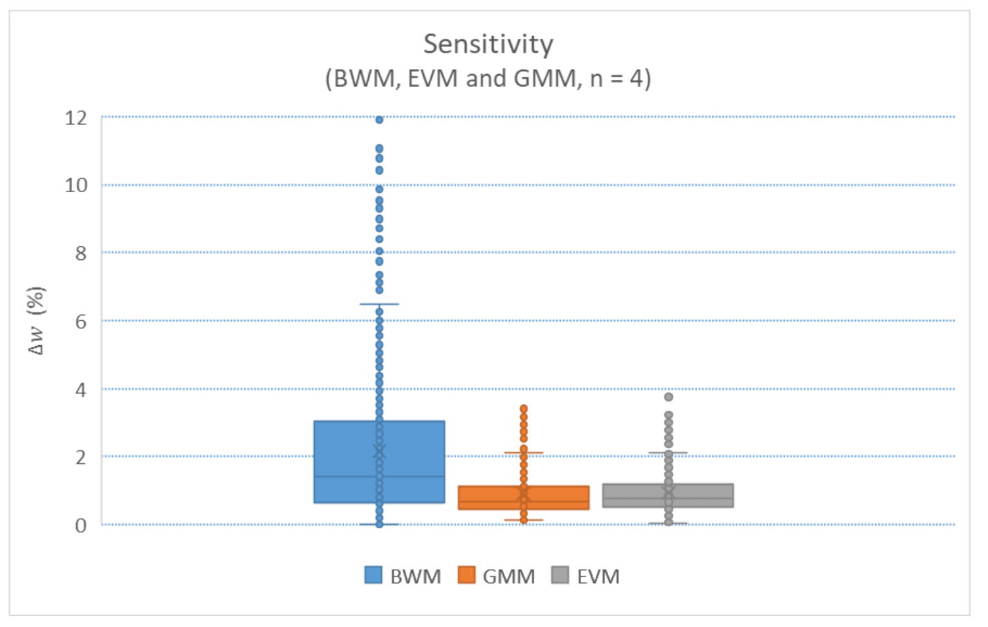
Our results, summarized in Table 1, indicate that the mean sensitivity decreases with the matrix size for all three prioritization methods; however, the sensitivity of the BWM is markedly larger than that of the GMM and EVM. In Figure 7, Figure 8 and Figure 9, it can be seen that while the sensitivity of more than 1% is rare for the GMM and EVM (for $n=6$), it is quite common for the BWM. A standard statistical tool for testing the equality of three or more means is the ANOVA (analysis of variance). However, the ANOVA requires an equality of variances, and from Table 1 and Figure 4, Figure 5 and Figure 6, it is clear that this assumption was violated. Bartlett’s test confirmed that variances in the sensitivity of all three methods were not equal (at $p=0$). Therefore, we applied Welch’s test instead, and the null hypothesis of sensitivity equality was rejected at the $p=0$ level (p was so small that MS Excel rounded the value to 0) for all $3\le n\le 8$. Since the BWM is “handicapped” by the lower number of pairwise comparisons required, we also performed Welch’s test for sensitivity equality of all three methods, where the sensitivity of the BWM was adjusted (decreased) by the factor $\frac{2n-3}{n(n-1)/2}$, corresponding to the number of pairwise comparisons required by the BWM and EVM/GMM, respectively; see also Figure 3. Even after the adjustment, the null hypothesis of equal sensitivity was rejected at $p=0$ for all examined n again. Interestingly, the two-sample t-test revealed that differences in the sensitivity of the GMM and EVM were statistically significant at the $p=0.01$ level only for $n\in \{6,8\}$.

As for order violation, its occurrence increased for all three methods as the matrix size n increased. In the case of $n=8$, the order violation occurrence was more likely (above 50%) than not, and in the case of the BWM, it was almost certain to happen (above 97%). This result for $n=8$ means that even the smallest possible deviation (or error) in one pairwise comparison on the input leads to a different ranking of objects in more than 50% cases. It is likely that for greater matrix sizes, this phenomenon will happen even more often; this therefore implies that the robustness of rankings of objects derived from pairwise comparisons by the BWM, EVM, and GMM is rather low, and the decision maker should take this into account. Differences in order violation occurrence (considered to be a binomial variable where either order violation happened or not) between all three methods were again tested for statistical significance. The null hypothesis that there is no difference between the BWM and GMM, and the BWM and EVM, was rejected at $p<{10}^{-10}$ for all n. Differences between the GMM and EVM were statistically significant at the $p=0.01$ level for $n\in \{5,6,7\}$, but not statistically significant at $p=0.01$ for $n\in \{3,4,8\}$.

5. Illustrative Application of Our Approach to Order Violation Evaluation

The study of Zabihi et al. [31] focused on developing a global information system (GIS)-based multiple-criteria decision making model for a citrus land suitability assessment. The authors selected five relevant criteria: elevation, maximum temperature, minimum temperature, slope angle, and rainfall. To determine the importance of criteria, the authors pairwise compared all criteria with the Saaty’s scale. The resulting pairwise comparison matrix is shown in

Table 2. A pairwise comparison matrix for the calculation of criteria weights for the citrus site selection (Table 4, Zabihi et al. [31]).

Sustainability Criterion	Elevation	Maximum Temperature	Minimum Temperature	Slope Angle	Rainfall
elevation	1	5	3	7	5
maximum	$1/5$	1	$1/3$	3	$1/2$
temperature
minimum	1/3	3	1	5	3
temperature
slope angle	$1/7$	$1/3$	$1/5$	1	$1/5$
rainfall	$1/5$	2	$1/3$	5	1

. By using the EVM, we obtained the vector of the weights of all criteria, and we ranked them from the most important to the least important as follows: elevation (weight $0.497$), minimum temperature ($0.242$), rainfall ($0.132$), maximum temperature ($0.087$), and slope angle ($0.041$). (Notice that the weights in parentheses slightly differ from the study of Zabihi et al. [31], perhaps due to numerical errors in [31].)

Since measurements or judgments are usually associated with errors, the question arises as to how stable the obtained ranking of the criteria is, or, in other words, is there an element (the so called critical element) in the PC matrix in Table 2 such that the minimal change of this matrix element leads to an order violation; i.e., a change in the ranking of all criteria?

Without loss of generality, we can examine all matrix elements in Table 2 (we denote the matrix as $C=\left[c_{ij}\right]$) larger than or equal to 1 (with the exception of diagonal elements):

•  Let us start with $c_{12}=5$. We change the value of 5 down by 1 scale unit (to 4), apply the EVM to find the priority vector and the ranking of all five criteria, and we get the following result: the ranking of elevation, minimum temperature, rainfall, maximum temperature, and slope angle remains unchanged. Next, we change the value of $c_{12}=5$ up by 1 unit (to 6), repeat the procedure, and find that the final ranking is unchanged again.
•  We take another matrix element larger than or equal to 1, namely $c_{13}=3$, and change it by 1 scale unit up and down. Again, the final ranking obtained by the EVM is unchanged in both cases.
•  We proceed with the remaining elements larger than or equal to 1, namely $c_{14}$, $c_{15}$, $c_{24}$, $c_{32}$, $c_{34}$, $c_{35}$, $c_{52}$, and $c_{54}$, and change each of them by 1 scale unit up and down. The final ranking obtained by the EVM remains unchanged in all cases.

We thus conclude that the pairwise comparison matrix given in Table 2 is “robust” in the sense that the ranking of the alternatives (elevation, minimum temperature, rainfall, maximum temperature, and slope angle) remains the same if one element of the matrix is changed by 1 scale unit up or down.

The pairwise comparisons presented in Table 2 were obtained by an expert team, and the EVM yielded the priority vector $w=(0.497,0.087,0.242,0.041,0.132)$. Taking these weights of the criteria into account, another expert team may pairwise compare the criteria’s importance as presented in

Table 3. A pairwise comparison matrix for the calculation of criteria weights for the citrus site selection by another expert team.

Sustainability Criterion	Elevation	Maximum Temperature	Minimum Temperature	Slope Angle	Rainfall
elevation	1	6	2	9	4
maximum	$1/6$	1	$1/3$	2	1
temperature
minimum	$1/2$	3	1	6	2
temperature
slope angle	$1/9$	$1/2$	$1/6$	1	$1/3$
rainfall	$1/4$	1	$1/2$	3	1

. Notice that Saaty’s consistency ratio of the PC matrix presented in Table 2 and Table 3 is $\mathit{CR}=0.055$ and $\mathit{CR}=0.007$, respectively; i.e., the PC matrix presented in Table 3 appears to be much more consistent than the original PC matrix presented in Table 2.

By applying the EVM to the PC matrix found in Table 3, we obtain the vector of the weights of the criteria. The ranking of the criteria is the same as above: elevation ($0.486$), minimum temperature ($0.256$), rainfall ($0.119$), maximum temperature ($0.093$), and slope angle ($0.045$).

Although the new pairwise comparison matrix, denoted as $C^{\prime }=\left[c_{ij}^{\prime }\right]$, shown in Table 3 is more consistent, a critical element can be found in it. In particular, by changing the value of the element $c_{25}^{\prime }=1$ by 1 scale unit up (to 2) and by using the EVM, we obtain the following weights and ranking of the criteria: elevation ($0.483$), minimum temperature ($0.255$), maximum temperature ($0.112$), rainfall ($0.106$), and slope angle ($0.045$). We can see that the change of the critical element $c_{25}^{\prime }$ by 1 scale unit, which is the smallest possible change of a PC matrix, caused order violation; i.e., it led to a different ranking of the criteria for citrus land suitability assessment. The sensitivity $△w_{\left(5\right)}^{\left(\mathit{EVM}\right)}=0.749$ was above the mean value $0.474$ (see Table 1) in this case. Knowing this, the decision maker should pay special attention to this particular PC comparison (or a measurement in general) to ensure its accuracy and to avoid a distortion of the final ranking. Our Monte Carlo simulations revealed that the frequency occurrence of critical elements increased with the increasing matrix size for all three priority deriving methods; see Table 1.

6. Conclusions

The aim of this paper was to provide a comparison of the sensitivity and order violation of three popular prioritization methods in pairwise comparisons: the Geometric Mean Method, the Eigenvalue Method, and the Best–Worst Method.

Our results suggest that the Best–Worst Method is statistically significantly more sensitive and more susceptible to order violation than the Geometric Mean Method and the Eigenvalue Method for $3\le n\le 8$ compared objects. On the other hand, the difference in sensitivity of the Geometric Mean Method and the Eigenvalue Method was found to be statistically insignificant in most cases.

Since both the GMM and EVM outperformed the BWM, and the differences in the GMM and EVM were rather small, both “standard” methods can equally be recommended as a suitable prioritization method with regard to sensitivity and order violation.

Further, we demonstrated how our approach can be used in practice for the evaluation of the stability of a ranking obtained by a given PC method. We came across a surprising finding that, with the increasing size of the PC matrix, the relative frequency of critical elements also increases.

Future research may focus on a comparison of extensions of the aforementioned methods aiming at interval pairwise comparisons or fuzzy pairwise comparisons.

References

- Brans, J.P.; Vincke, P. A preference ranking organisation method: The PROMETHEE method for MCDM. Manag. Sci. 1985, 31, 647–656. [Google Scholar] [CrossRef] [Green Version]
- Figueira, J.; Greco, S.; Ehrgott, M. Multiple Criteria Decision Analysis: State of the Art Surveys; Springer Science + Business Media, Inc.: New York, NY, USA, 2005. [Google Scholar]
- Hansen, P.; Ombler, F. A new method for scoring additive multi-attribute value models using pairwise rankings of alternatives. J. Multi-Criteria Decis. Anal. 2008, 15, 87–107. [Google Scholar] [CrossRef]
- Koksalan, M.M.; Wallenius, J.; Zionts, S. Multiple Criteria Decision Making: From Early History to the 21st Century; World Scientific Publishing: Singapore, 2011. [Google Scholar]
- Mardani, A.; Jusoh, A.; Nor, K.M.D.; Khalifah, Z.; Zakwan, N.; Valipour, A. Multiple criteria decision-making techniques and their applications–a review of the literature from 2000 to 2014. Econ. Res.-Ekon. Istraz. 2015, 28, 516–571. [Google Scholar] [CrossRef]
- Roy, B. Classement et choix en presence de points de vue multiples (la methode ELECTRE). Rev. D’Inform. Rech. Oper. (RIRO) 1968, 8, 57–75. [Google Scholar]
- Saaty, T.L. A Scaling Method for Priorities in Hierarchical Structures. J. Math. Psychol. 1977, 15, 234–281. [Google Scholar] [CrossRef]
- Saaty, T.L. Analytic Hierarchy Process; McGraw-Hill: New York, NY, USA, 1980. [Google Scholar]
- Saaty, T.L. Fundamentals of Decision Making; RWS Publications: Pittsburgh, PA, USA, 1994. [Google Scholar]
- Vaidya, O.; Kumar, S. Analytic Hierarchy Process: An Overview of Applications. Eur. J. Oper. Res. 2006, 169, 1–29. [Google Scholar] [CrossRef]
- Crawford, G.B. The geometric mean procedure for estimating the scale of a judgement matrix. Math. Model. 1987, 9, 327–334. [Google Scholar] [CrossRef] [Green Version]
- Rezaei, J. Best-worst multi-criteria decision-making method. Omega 2015, 53, 40–57. [Google Scholar] [CrossRef]
- Abadia, F.A.; Sahebib, I.G.; Arabc, A.; Alavid, A.; Karachi, H. Application of best-worst method in evaluation of medical tourism development strategy. Decis. Sci. Lett. 2018, 7, 77–86. [Google Scholar] [CrossRef]
- Ahmadi, A.B.; Kusi-Sarpong, S.; Rezaei, J. Assessing the social sustainability of supply chains using Best Worst Method. Resour. Conserv. Recycl. 2017, 126, 99–106. [Google Scholar] [CrossRef]
- Chang, M.-H.; Liou, J.J.H.; Lo, H.-W. A Hybrid MCDM Model for Evaluating Strategic Alliance Partners in the Green Biopharmaceutical Industry. Sustainability 2019, 11, 4065. [Google Scholar] [CrossRef] [Green Version]
- Gupta, H.; Barua, M.K. Supplier selection among SMEs on the basis of their green innovation ability using BWM and fuzzy TOPSIS. J. Clean. Prod. 2017, 152, 242–258. [Google Scholar] [CrossRef]
- Rezaei, J.; Nispeling, T.; Sarkis, J.; Tavasszy, L. A supplier selection life cycle approach integrating traditional and environmental criteria using the best worst method. J. Clean. Prod. 2016, 135, 577–588. [Google Scholar] [CrossRef]
- Setyono, R.P.; Sarno, R. Vendor Track Record Selection Using Best Worst Method. In Proceedings of the 2018 International Seminar on Application for Technology of Information and Communication, Semarang, Indonesia, 21–22 September 2018; pp. 41–48. [Google Scholar]
- Ajrina, A.S.; Sarno, R.; Hari Ginardi, R.V. Comparison of AHP and BWM Methods Based on Geographic Information System for Determining Potential Zone of Pasir Batu Mining. In Proceedings of the 2018 International Seminar on Application for Technology of Information and Communication, Semarang, Indonesia, 21–22 September 2018; pp. 453–457. [Google Scholar]
- Haseli, G.; Sheikh, R.; Sankar Sana, S. Base-criterion on multi-criteria decision-making method and its applications. Int. J. Manag. Sci. Eng. Manag. 2020, 15, 79–88. [Google Scholar] [CrossRef]
- Cacuci, D.G.; Ionescu-Bujor, M.; Navon, M. Sensitivity and Uncertainty Analysis, Vol. II: Applications to Large-Scale Systems; Chapman & Hall/CRC: Boca Raton, FL, USA, 2005. [Google Scholar]
- Helton, J.C.; Johnson, J.D.; Salaberry, C.J.; Storlie, C.B. Survey of sampling based methods for uncertainty and sensitivity analysis. Reliab. Eng. Syst. Saf. 2006, 91, 1175–1209. [Google Scholar] [CrossRef] [Green Version]
- Saltelli, A.; Chan, K.; Scott, M. (Eds.) Sensitivity Analysis; Wiley Series in Probability and Statistics; John Wiley and Sons: New York, NY, USA, 2000. [Google Scholar]
- Saltelli, A. Sensitivity Analysis for Importance Assessment. Risk Anal. 2002, 22, 579–590. [Google Scholar] [CrossRef] [PubMed]
- Czitrom, V. One-Factor-at-a-Time Versus Designed Experiments. Am. Stat. 1999, 53, 126–131. [Google Scholar]
- Ramík, J. Ranking Alternatives by Pairwise Comparisons Matrix and Priority Vector. Sci. Ann. Econ. Bus. 2017, 64, 85–95. [Google Scholar] [CrossRef]
- Brunelli, M.; Rezaei, J. A multiplicative best-worst method for multi-criteria decision making. Oper. Res. Lett. 2019, 47, 12–15. [Google Scholar] [CrossRef]
- Rezaei, J. Best-worst multi-criteria decision-making method: Some properties and a linear model. Omega 2016, 64, 126–130. [Google Scholar] [CrossRef]
- Best Worst Method: BWM Solvers. Available online: https://bestworstmethod.com/software/ (accessed on 31 January 2021).
- Perzina, R.; Mazurek, J.; Ramík, J.; Bartl, D. Data for `A Numerical Comparison of the Geometric Mean Method, the Eigenvalue Method, and the Best-Worst Method’, Mendeley Data, v1 (2021). Available online: https://data.mendeley.com/datasets/svdjzz2nk6/draft?a=a1fbe712-5d57-44da-b79d-0d4d56eaad2d (accessed on 31 January 2021).
- Zabihi, H.; Alizadeh, M.; Kibet Langat, P.; Karami, M.; Shahabi, H.; Ahmad, A.; Nor Said, M.; Lee, S. GIS Multi-Criteria Analysis by Ordered Weighted Averaging (OWA): Toward an Integrated Citrus Management Strategy. Sustainability 2019, 11, 1009. [Google Scholar] [CrossRef] [Green Version]