Regression Methods Based on Nearest Neighbors with Adaptive Distance Metrics Applied to a Polymerization Process

Abstract

Empirical models based on sampled data can be useful for complex chemical engineering processes such as the free radical polymerization of methyl methacrylate achieved in a batch bulk process. In this case, the goal is to predict the monomer conversion, the numerical average molecular weight and the gravimetrical average molecular weight. This process is characterized by non-linear gel and glass effects caused by the sharp increase in the viscosity as the reaction progresses. To increase accuracy, one needs more samples in the areas with higher variation and this is achieved with adaptive sampling. An extensive comparative study is performed between three regression algorithms for this chemical process. The first two are based on the concept of a large margin, typical of support vector machines, but used for regression, in conjunction with an instance-based method. The learning of problem-specific distance metrics can be performed by means of either an evolutionary algorithm or an approximate differential approach. Having a set of prototypes with different distance metrics is especially useful when a large number of instances should be handled. Another original regression method is based on the idea of denoising autoencoders, i.e., the prototype weights and positions are set in such a way as to minimize the mean square error on a slightly corrupted version of the training set, where the instances inputs are slightly changed with a small random quantity. Several combinations of parameters and ways of splitting the data into training and testing sets are used in order to assess the performance of the algorithms in different scenarios.

1. Introduction

There are many situations when one needs to discover a relationship between one or more independent variables, the inputs, and one real-valued dependent variable, i.e., the output—from data samples. This type of problem is known as regression, and a large number of algorithms have been proposed by researchers. Among the most popular ones, one can mention neural networks, support vector machine regression (ε-SVR, ν-SVR), decision trees (M5P, random forest, REPTree) or methods based on instances (k-nearest neighbor) or rules (M5, decision table).

The Large Margin Nearest Neighbor for Regression (LMNNR) algorithm [1] has been used in several studies so far for a variety of applications and its performance has been compared to that of classic regression methods implemented in the popular collection of machine learning algorithms Weka [2]. Thus, in [1,3], it was used for the prediction of corrosion resistance of some alloys containing titanium and molybdenum, widely used in dental applications. The material corrosion was quantified by the polarization resistance of the TiMo alloys.

The LMNNR algorithm was also applied in a different field, that of predicting students’ performance based on their active use of social media tools during the learning process [4,5]. The training data were collected over six winter semesters in consecutive years, from a total of 343 students. Almost 19,000 social media contributions were recorded and used to compute 14 numeric features for each student. Based on these, the final grade was predicted.

The results of LMNNR have been generally shown to be better than those of the other regression algorithms used for comparison. Although more variants for model training and model representation have been proposed, its main disadvantage is that its sensitivity to local optimal often requires multiple runs, and thus increases the training time.

In [6], a modified nearest-neighbor regression method (kNN) is proposed for modeling the photocatalytic degradation of the Reactive Red 184 dye for which insufficient data are available. It can handle partial information without “filling in” additional computed values (mean values) or ignoring the incomplete instances. In the case of the photocatalytic degradation process, the kNN method recorded correlations of over 0.9.

A study based on an adaptive regression model appropriate for cases with insufficient or missing data was also performed in [7]. Its aim was to investigate the electrochemical behavior of ZrTi alloys in artificial saliva. This method has only one internal parameter whose optimal value is found automatically.

The prediction of the sublimation rate of naphthalene in various working conditions was studied in [8]. Different regression methods were applied and the performance of the original Large Margin Nearest Neighbor Regression algorithm (LMNNR) proved superior to those of other classical ones.

In the present study, three regression variants are applied for the free radical polymerization of methyl methacrylate (MMA) achieved in a batch bulk process. The first two variants are based on LMNNR trained either with an evolutionary algorithm or by gradient descent, where the derivatives are approximated by means of the central difference method. This is the first time that LMNNR has been applied for this process. Its difficulty is caused by the gel effect, corresponding to an abrupt conversion and molecular mass jump which may be missed by less accurate regression techniques. The third variant is a new, original algorithm named Nearest Neighbor Regression with Adaptive Distance Metrics Trained by Multiple Point Hill Climbing on Noisy Training Set Error (RADIAN) which is not based on the concept of a large margin but is inspired by denoising autoencoders used in deep learning [9], where the input data are slightly corrupted, and the model is forced to learn the correct data from the corrupted version in order to prevent overfitting.

Regarding the results obtained for the polymerization of MMA with the above-mentioned methods, it is important to point out not only that they are very good, but also that they follow previous sustained efforts, made with different other methods whose results were inferior to those reported here.

2. Dataset

In order to test the functionality of the regression algorithms mentioned in the article, a real-world problem, namely the free radical polymerization of methyl methacrylate, was chosen as a case study. Two reasons justify this choice: the complexity of the process, so the difficulties in modeling and also the fact that our group has tried different modeling methods for this system, so that the obtained results can be compared with those reported in this paper.

Polymerization reactions present some difficulties in modeling and optimization actions, because of their specific features, as well as the general characteristics of the chemical processes. Reactions are complex and their mechanism is often not fully known. Developing accurate models implies precise knowledge of the phenomenology of the process, as well as of the physical and chemical laws that govern them. A series of approximations are often needed, influencing the accuracy of the model results. In addition, the complexity of the mathematical models causes supplementary difficulties regarding the solution mode and the time required for this operation, given the requirement of using the models in online optimal control procedures. Under these conditions, empirical models that use input–output data sets can be considered a preferable alternative to mechanistic models, both in terms of working methodology and the accuracy of results.

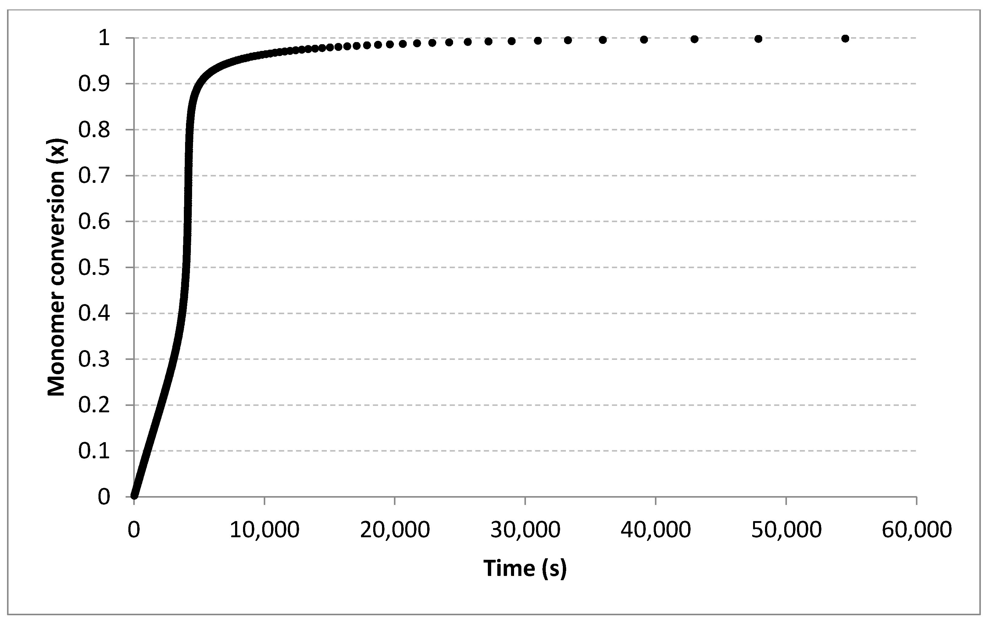
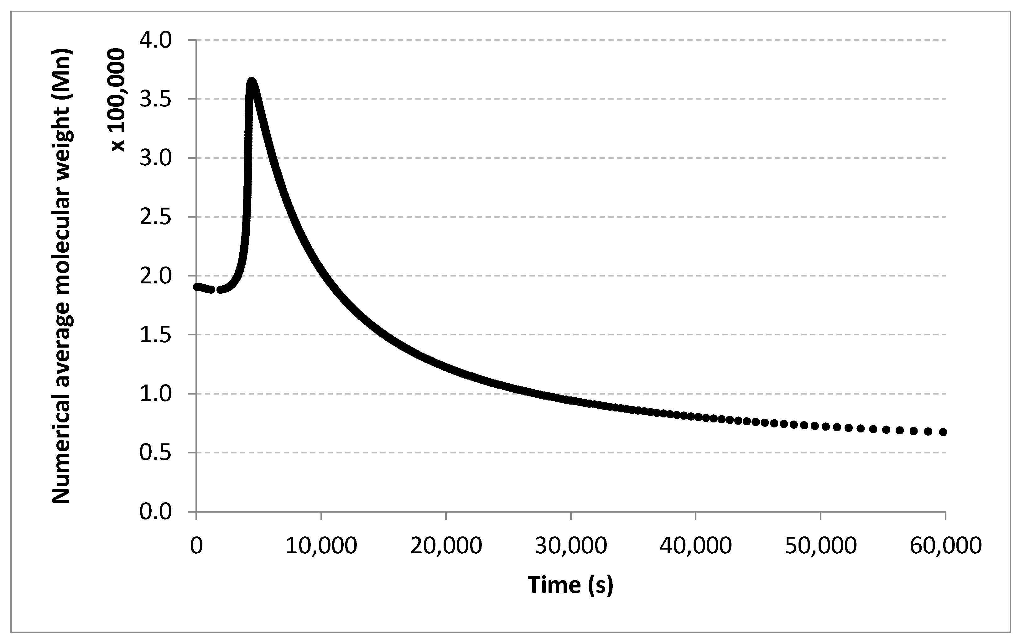
The free radical polymerization is characterized by diffusion-controlled effects. As the viscosity of the reaction mass increases, there is a sudden increase in the conversion and molecular masses, as a result of the diffusion difficulties encountered by the increasing macroradicals. The so-called glass and gel phenomena appear as a result of decreasing the values of the propagation and termination rate constants. The result of the manifestation of controlled diffusion phenomena is the end of polymerization reaction before the complete consumption of the reactants.

From the point of view of the modeling action, the diffusion-controlled effects are more difficult to model, especially since their phenomenology is not completely elucidated. Various models have been proposed, with a pronounced empirical character, e.g., [10] or [11], but their efficiency and application are limited. In addition, they have a pronounced empirical character, including many constants that can be determined by matching the experimental data, which means their dependence on each set of reaction conditions (temperature, concentrations of reactants etc.).

Some of the reasons listed above involve the need to apply modeling methods leading to better results, a variant being represented by neural networks, applied in the form of different methodologies. The following examples belong to our working group and have the role of justifying the new methodology described and applied in this paper and highlighting the results obtained, better than in the previous approaches. Therefore, several previous results will be presented.

The first series of attempts [12,13] implied the design of neural networks of feed-forward type, by the method of successive trials, to correlate the conversion and molecular masses with the reaction conditions. If satisfactory results were obtained for the conversion, for the molecular masses, especially for the average gravimetric molecular mass, the accuracy was below the minimum required. A more complex approach, which led to better results [14] was based on combining a simplified phenomenological model with neural networks, obtaining hybrid models. Several modeling modalities were considered, namely the neural networks have replaced different parts of the model—in general the parts difficult to model due to diffusion-controlled phenomena. The results obtained were much better than the models represented by single neural networks, but also not very satisfactory for gravimetrical molecular weight.

Another example is represented by the use of a hybrid stacked recurrent neural model for a batch MMA polymerization reactor [15]. Stacked recurrent neural networks are developed for modeling the gel effect, and they are associated with a simplified phenomenological model to obtain a complete model, improved in performance and robustness because of the multiple neural networks included in the model. The results are satisfactory, but there is still room for improvement.

Regarding the mentioned methods, their complexity should be noted, deriving from the need to determine optimal neural networks and their combination with other instruments.

3. Standard and Large Margin Nearest Neighbor Methods

3.1. Standard Nearest Neighbor-Based Regression

Learning methods based on instances are among the simplest machine learning algorithms but provide remarkable results for a large variety of tasks, especially when the training data are not affected by noise and when there is a proper correspondence between the dimensionality of the problem and the size of the training dataset. For regression problems, the goal is to approximate a function between a real-valued dependent variable given one or more independent variables based on a training set of examples $S=\left\{x_1,\dots ,x_m\right\}$. In this case, k-Nearest Neighbor (kNN), the value of a query instance can be computed as the mean value of the function of the nearest neighbors:

$$\tilde{f}(x)=\frac{1}{k}{\displaystyle \sum _{x^{\prime }\in N(x)}f(x^{\prime })},$$

(1)

where $N(x)\subseteq S$ is the set of the closest k instances (i.e., neighbors) of x in the dataset S.

Nevertheless, finding the most appropriate value of k may not be straightforward, so another possibility is to give weights to the training instances such that the weights of each neighbor depend on the distance to the query point:

$$\tilde{f}(x)=\frac{1}{z}{\displaystyle \sum _{x^{\prime }\in S}{w}_d(x,x^{\prime })\cdot f(x^{\prime })},$$

(2)

where z is a normalization factor. The inverse of the square Euclidean distance is often used to determine these weights:

$$w_d(x,x^{\prime })=\frac{1}{d{(x,x^{\prime })}^2}=\frac{1}{{\displaystyle \sum _{i=1}^n{\left(x_i-{x^{\prime }}_i\right)}^2}}.$$

(3)

kNN works well for many problems, especially when the number of instances is large, the dimensionality of the data is not too big and there is little noise in the data. A crucial component of such a method is the distance metric, because the new instances are evaluated based on their similarity to the training instances. The Euclidean distance is the most common, but different particularizations of the general Minkowski distance, such as the Manhattan distance, or more advanced distance metrics such as the exponentially negative distance function, can also be used [16,17].

However, the standard approach does not take into account problem-specific information, but only considers some general optimizations, such as choosing the best number of neighbors k by cross-validation, or normalizing instance values on each dimension. There is little problem-specific knowledge embedded into the method.

3.2. Large Margin Nearest Neighbor for Classification

To increase performance, researchers have tried to find various methods to tune the distance metric for the different problems being considered. Problem-specific distance metrics have been recognized as capable of significantly improving the results. This process is known as distance metric learning. In general, distance metric learning can be defined as finding a linear transformation $x^{\prime }=Lx$, which transforms the distance between two vectors x_i and x_j to:

$$d_L(x_i,x_j)={\Vert L\left(x_i-x_j\right)\Vert }_2^{}.$$

(4)

Since all operations in classification or regression based on k nearest neighbors can be performed with square distances, a transformation based on a square matrix may be easier to use: M = L^T L, such that the square distance becomes:

$$d_M(x_i,x_j)={\left(x_i-x_j\right)}^{T}M\left(x_i-x_j\right).$$

(5)

In the following algorithms, we investigate the use of the concept of “large margins”, well known from the support vectors machines (SVM). We adapt it for regression problems, from ideas pertaining to classification problems.

As presented above, a problem-specific distance metric means that the actual distance is multiplied by a matrix that is computed from the training set, resulting in warping the problem space such that, e.g., for a classification problem, the instances that belong to the same class are closer together than the instances that belong to different classes, and also possibly insuring an arbitrary separation margin between classes.

The idea of a large margin was transferred from the SVM domain to kNN to perform classification tasks in the Large-Margin Nearest Neighbor algorithm (LMNN) [18]. The optimization problem is solved by semi-defined programming and the method can be extended to be invariant to multivariate polynomial transformations [19].

In [18], the M matrix is computed such that the distance between an instance $x_i$ and its k neighbors from the same class $x_j$ (named a “target”) is minimized. However, this is not sufficient, because reducing all distances to 0 would satisfy this condition. The second constraint is that the distance between instance $x_i$ and its k neighbors from a different class $x_l$ (named an “imposter”) is maximized. An additional idea is that the minimum distance to an imposter should be greater than any distance to a target plus some additional value:

$$d_M(x_i,x_l)\ge 1+d_M(x_i,x_j),$$

(6)

where 1 is arbitrary and has the significance of an imposed margin between the classes.

These two constraints are conflicting; therefore the authors introduce some weights, following an analogy from physics regarding forces of attraction and repulsion. Ultimately, in their examples, they consider the weights of the constraints to be equal.

3.3. Large Margin Nearest Neighbor for Regression

For a regression problem, the same concept can be applied by taking into account the actual real values of the output instead of discrete class values. This is the main idea of the Large Margin Nearest Neighbor for Regression (LMNNR) algorithm [3]. The distance metric is computed by optimizing an objective function composed of two conflicting criteria which can be given different weights in the final objective functions or can be scaled using different functions [5]. LMNNR also allows that different matrices can be used for different regions of the problem space, identified by special points known as prototypes. The locations of the prototypes can be statically initialized, e.g., by using a clustering algorithm such as k-means [3] or dynamically learned, together with the distance metrics [1].

The optimization of the objective function can be carried out either using an evolutionary algorithm [3], which can be rather slow, but has a good chance of finding a global optimum, or by using an approach based on gradient descent [1], which is much faster, but may need several different runs in order to converge to a good solution.

We assume that M is a diagonal matrix. This has the advantage that the m_ii elements can be interpreted as the weights of the inputs. Because of the definition $M=L^{T}L$, M must be symmetrical and positive semidefinite. Using M, Equation (3) is still valid, but becomes:

$$w_{d_M}(x,x^{\prime })=\frac{1}{d_M(x,x^{\prime })}=\frac{1}{{\displaystyle \sum _{i=1}^n{m}_{ii}\cdot {\left(x_i-{x^{\prime }}_i\right)}^2}}.$$

(7)

In this formulation, there is a single M for all instances. However, it is possible to use different distance metrics for different groups of instances identified by special center points which we call prototypes. Each prototype P can have its own matrix M^P. When calculating the weight of the distance for a new point, an instance will use the weights for the closest prototype $m_{ii}^P$ instead of $m_{ii}^{}$ in Equation (7). The optimization problem assumes the minimization of the following objective function:

$$F={\varphi }_1\left(F_1\right)+{\varphi }_2\left(F_1\right)+{\varphi }_3\left(F_3\right),$$

(8)

in which ${\varphi }_i(\cdot )$ are custom functions, e.g., in the simplest case, ${\varphi }_i(x)=w_i\cdot x$.

We will use the following notations when defining the components of F: $d_{ij}=d_M\left(x_i,x_j\right),$ $d_{ik}=d_M\left(x_i,x_k\right),$ $g_{ij}=\left|f(x_i)-f(x_j)\right|$ and $g_{ik}=\left|f(x_i)-f(x_k)\right|$.

Thus, the first criterion is:

$$F_1={\displaystyle \sum _{i=1}^n{\displaystyle \sum _{j\in N(i)}{d}_{ij}}}\cdot \left(1-g_{ij}\right),$$

(9)

where N(i) is the set of the k nearest neighbors for an instance i (e.g., k = 3). It ensures that the closer the instances in the input space, the closer their output values should be. Conversely, distant instances should have different output values.

The second criterion is:

$$F_2={\displaystyle \sum _{i=1}^n{\displaystyle \sum _{j\in N(i)}^{}{\displaystyle \sum _{l\in N(i)}^{}\Delta d_{ijl}\cdot \Delta y_{ijl}\cdot \left(1+\frac{1}{\Delta d_{ijl}\cdot \Delta y_{ijl}+\epsilon }\right)}}},$$

(10)

where $\Delta d_{ijl}=\max \left(d_{il}-d_{ij},0\right)$, $\Delta y_{ijl}=\max \left(g_{ij}-g_{il},0\right)$ and where ε is a small positive real number. This criterion imposes penalties when the “proximity order” is violated, i.e., when g_ij < g_ik but d_ij > d_ik. It attempts to minimize the proximity order breaks [20], i.e., the cases when g_ij < g_ik but d_ij > d_ik. Given an instance i, the optimization reduces the number of situations when another instance l is farther than another one j, but its output value is closer to that of i than the output value of j.

The third criterion can be optionally used for regularization:

$$F_3={\displaystyle \sum _{j=1}^{n_p}{\displaystyle \sum _{i=1}^{n_i}{m}_{ii}(j)}}.$$

(11)

From our experimental studies, we empirically found that a good objective function is:

$$F=F_1+\sqrt{F_2},$$

(12)

because F₂ is usually larger than F₁. Additionally, it was found that regularization was not needed for the presented case studies.

In the following sections, we will give a complete description of two algorithms which implement the LMNNR idea, together with a third algorithm which relies on a different principle.

4. Description of the Algorithms

4.1. Large Margin Nearest Neighbor Regression Trained with an Evolutionary Algorithm (LMNNR-EA)

The first method solves the problem defined by Equation (7) by means of an evolutionary algorithm. The advantages of applying an evolutionary algorithm for optimization is that prototypes, with different weight values, can be used instead of a single set of weights. The prototype positions are precomputed using the k-means algorithm. Since the resulting clusters tend to be (hyper-)spherical, the method is suitable for the complex problems addressed, as the distances are computed with different variants of Euclidean metrics.

4.2. Large Margin Nearest Neighbor Regression Trained with Approximate Gradient Descent (LMNNR-AGD)

Gradient descent optimization is a more-or-less de facto standard for recent machine learning methods, especially (deep) neural networks. It is usually faster than evolutionary optimization, however it is sensitive to the initial value estimate which may cause it to converge to a local optimum.

For the problems addressed here, the standard gradient descent method cannot be applied for several reasons. First, the objective function is not continuous because of the max function in Equation (10). In addition, for the expressions of the components of the objective functions defined by Equations (9) and (10) the analytical form of the gradient is difficult to express. Thirdly, the positions of the prototypes need to be optimized simultaneously with the weights.

In the evolutionary approach, the space of the problem has proved to be large enough so that finding the position of the prototypes is not feasible, and that is why the compromise solution using clustering was used. With gradient-based optimization this becomes possible. Still, when the position of the prototypes changes, the neighbor instances also change. Therefore, the objective function is calculated differently, considering different or similar instances, with different weights. This is also difficult to express in the analytical formulation of the gradient.

Thus, we decided to use an approximate differential method, following the definition of the central difference for the derivative. That is, for a very small value ε:

$$f^{\prime }(x)\approx \frac{f(x+\epsilon )-f(x-\epsilon )}{2\epsilon },$$

(13)

in which the truncation error is O(ε²).

The value of the step size γ is very important for the convergence speed. Therefore, it can be dynamically adjusted, so that it is higher at the beginning and decreasing as the algorithm approaches the solution. It was considered that the value of the step starts from about 1 and then decreases with the number of iterations, following a quadratic reciprocal evolution, but preventing it from going below 0.1:

$${\gamma }_n=\max \left(\frac{1}{a+bn+c{n}^2},0.1\right),$$

(14)

where n is the number of iterations, and the values of the a, b and c parameters can be set to adjust the slope of the curve.

4.3. Nearest Neighbor Regression with Adaptive Distance Metrics Trained by Multiple Point Hill Climbing on Noisy Training Set Error (RADIAN)

The Nearest Neighbor Regression with Adaptive Distance Metrics Trained by Multiple Point Hill Climbing on Noisy Training Set Error (RADIAN) algorithm is not based on the concept of a large margin but is inspired by a technique used in deep learning, i.e., denoising autoencoders. This is a type of deep network that learns the presented data itself, but transfers it through an intermediate layer, usually a bottleneck with a number of neurons smaller than the dimensionality of the problem, so this layer will capture the essential characteristics of the data. In order to prevent the phenomenon of overfitting, the input data are slightly corrupted and the autoencoder is forced to learn the correct data from the corrupted version.

The overall concept of learning a distance metric and the distribution of the prototypes in the problem space are the same as for the previous algorithms. However, the prototype weights and positions are set so as to minimize the mean square error on a slightly corrupted version of the training set, where the instances inputs are slightly changed with a small random quantity:

$$x_{ij}^{\prime }=x_{ij}+2(r-1/2)\cdot \epsilon ,$$

(15)

where x_ij is the value of the data, r is a random uniform number in the [0, 1) interval and ε is a small number, e.g., ε = 0.001.

The minimization is performed here by multiple point hill climbing. This method combines the approach of gradient descent with the search for a solution from multiple initial points, similar in a way to the parallel search performed by evolutionary algorithms. In standard hill climbing, several neighbors of the current point are generated, e.g., by an equation similar to (15). The point with a better (lower) objective function is selected as the new current point and the procedure is repeated for a number of steps. However, this behavior is similar to gradient descent, which is prone to local optima. Therefore, the search is performed from multiple starting points, so the probability of starting in a neighborhood of the global optimum is increased.

An idea for future investigation is to initialize the positions of the prototypes using the k-means clustering algorithm, instead of random initialization, such that they fill the problem space more uniformly.

From the initial results, it seems that this simple algorithm outperforms the other two for the problems under study.

5. Modeling Methodology

The free radical polymerization of methyl methacrylate achieved in a batch bulk process has non-linear gel and glass effects, i.e., regions where the values of the output parameters have a high variation. The data necessary for the application of the regression methods were obtained on a simulator [21], and their number is very large if we consider the faithful rendering of the gel effect corresponding to an abrupt conversion and molecular mass jump. Using constant sampling may miss these regions. In order to address this problem, an adaptive sampling technique was devised [22], which can select more samples around the critical regions. This algorithm first computes the local differences between successive points in the output function. This has the same meaning as a derivative. Then, it uses a running sum to determine whether the next point will be sampled. In regions with approximately constant values, the derivative is small, therefore the space between the sampled points will be larger. In regions with high variation, the derivative will be higher, and thus more points will be sampled. A number of points between 300 and 400 were obtained for all modeled parameters, instead of thousands of data when a constant step is applied. Monomer conversion (x), numerical average molecular weight (M_n), gravimetrical average molecular weight (M_w) are determined as function of reaction conditions (initiator concentration I₀, temperature T and time t).

Figure 1 and Figure 2 show two examples of applying the adaptive procedure for two of the considered outputs, x and M_n. The input conditions of the reaction are I₀ = 15 mol/m³ and T = 343 K.

6. Results and Discussion

In a previous study [22] we compared the results of several well-known algorithms from the Weka collection [2] with those of LMNNR for the three formulated problems, i.e., the conversion, average numerical and gravimetric molecular weights. The algorithms considered from Weka were: kNN, random forest, REPTree, M5 rules, additive regression, ε-SVR and ν-SVR, each with different values for their parameters. The data were split into 2/3 for training and 1/3 for testing.

Table 1. Performance of the best Weka algorithm for the monomer conversion (x), numerical average molecular weight (M_n) and gravimetrical average molecular weight (M_w) vs. Large Margin Nearest Neighbor for Regression (LMNNR).

Algorithm	Training x	Testing x	Training Mn	Testing Mn	Training Mw	Testing Mw
Random forest with 100 trees	0.999800	0.999800	0.999400	0.998600	0.999800	0.999600
LMNNR	1	0.999953	1	0.999638	1	0.999816

presents a concise comparison between the best classical algorithm (random forest) and LMNNR (with one prototype, five optimization neighbors and five regression neighbors) in terms of the coefficient of determination (R²) obtained for both the training and testing sets.

The fact that LMNNR obtains a perfect correlation for the training set is not surprising, since it is an instance-based method. It is, however, commendable that it outperforms the best Weka algorithm on the testing set. Therefore, in the present study, we focus only on the results of LMNNR in two variants and the newly introduced algorithm RADIAN and perform a comprehensive experimental study with different settings regarding the distribution of data and the parameters of the algorithms.

In order to assess the performance of the algorithms, cross-validation was used. The most common method is to split the data into ten groups (or bins) and use nine groups for training and one group for testing, and repeat the process ten times, every time with a different test group. In this study, in order to assess different aspects of the learning process, we use three cross-validation variants:

• Standard cross-validation with 10 groups, and in each step the data are split 90% for training and 10% for testing;
• Cross-validation with three groups, and in each step the data are split 67% for training and 33% for testing: this is similar to the simpler 2/3–1/3 split (e.g., used in [22], but more relevant statistically. This is a means to roughly compare results to those obtained in the previous work. However, a direct comparison is not possible;
• A cross-validation-like procedure with 10 groups, and in each step the data are split 10% for training and 90% for testing. This scenario is used to assess the generalization capability of the models more “aggressively”.

In terms of the parameters used for the algorithms, two settings were used, as displayed in

Table 2. The settings of the three regression algorithms. LMNNR-EA: Large Margin Nearest Neighbor Regression Trained with an Evolutionary Algorithm; LMNNR-AGD: Large Margin Nearest Neighbor Regression Trained with Approximate Gradient Descent; RADIAN: Nearest Neighbor Regression with Adaptive Distance Metrics Trained by Multiple Point Hill Climbing on Noisy Training Set Error.

	Algorithm 1: LMNNR-EA	Algorithm 2: LMNNR-AGD	Algorithm 3: RADIAN
Setting 1	No. groups = 10 No. prototypes = 2 No. regression neighbors = 3 No. optimization neighbors = 3 No. trials = 20 Population size = 40 Min. gene value = 0.001 Max. gene value = 10 Tournament size = 2 Crossover rate = 0.95 Mutation rate = 0.05 No. generations = 500	No. groups = 10 No. prototypes = 2 No. regression neighbors = 3 No. optimization neighbors = 3 No. trials = 20 Epsilon = 0.000001 Learning rate = 0.1 Dynamic learning rate = 0 Max. gradient descent steps = 1000	No. groups = 10 No. prototypes = 2 No. starting points = 20 No. regression neighbors = 5 No. hill-climbing steps = 30 No. hill-climbing neighbors = 20 Training set noise = 0.001 Hill-climbing noise = 0.01 Noise on output = 1
Setting 2	No. groups = 10 No. prototypes = 1 No. regression neighbors = 3 No. optimization neighbors = 3 No. trials = 10 Population size = 30 Min. gene value = 0.001 Max. gene value = 10 Tournament size = 2 Crossover rate = 0.95 Mutation rate = 0.05 No. generations = 100	No. groups = 10 No. prototypes = 1 No. regression neighbors = 3 No. optimization neighbors = 3 No. trials = 10 Epsilon = 0.000001 Learning rate = 0.1 Dynamic learning rate = 0 Max. G.D. steps = 200	No. groups = 10 No. prototypes = 1 No. starting points = 10 No. regression neighbors = 3 No. hill-climbing steps = 10 No. hill-climbing neighbors = 10 Training set noise = 0.001 Hill-climbing noise = 0.01 Noise on output = 1

:

• Setting 1: the parameters allow for greater, more general search capabilities, the values are larger, but this leads to a longer execution time;
• Setting 2: the values of the parameters are smaller. This setting allows us to see whether a shorter execution time can still provide acceptable results.

Table 3. The results of the algorithms with setting 1. MSE: mean squared error; r: coefficient of correlation.

	x		Mn		Mw
	r	MSE	r	MSE	r	MSE
Large training sets (90–10% data split)
Algorithm 1	0.999425	0.000124	0.999466	5.0707403	0.999459	78.1390448
Algorithm 2	0.999667	0.000074	0.999499	4.7406073	0.999680	46.6716341
Algorithm 3	0.999527	0.000120	0.999349	6.1569147	0.999396	79.0907101
Small training sets (10–90% data split)
Algorithm 1	0.962001	0.007573	0.987506	11.71332089	0.960302	566.565343
Algorithm 2	0.946293	0.010619	0.988202	11.08952839	0.959521	578.709620
Algorithm 3	0.91255	0.017117	0.986627	12.64085094	0.952598	574.958058

and

Table 4. The results of the algorithms with setting 2.

	x		Mn		Mw
	r	MSE	r	MSE	r	MSE
Large training sets (90–10% data split)
Algorithm 1	0.999644	0.000080	0.999469	5.0488433	0.999548	66.0130052
Algorithm 2	0.999665	0.000075	0.999503	4.6982778	0.999667	48.5893648
Algorithm 3	0.999663	0.000078	0.999345	6.1986015	0.998214	66.1359322
Small training sets (10–90% data split)
Algorithm 1	0.958308	0.008293	0.987379	11.889027	0.961123	555.051717
Algorithm 2	0.944513	0.010950	0.988040	11.244562	0.962062	541.849968
Algorithm 3	0.920547	0.015464	0.982747	16.316099	0.957143	550.783154
Average training sets (67–33% data split)
Algorithm 1	0.998997	0.000222	0.999171	7.843631	0.999286	10.425242
Algorithm 2	0.999017	0.000216	0.999197	7.587175	0.999471	17.444913
Algorithm 3	0.999004	0.000221	0.999191	7.634568	0.998949	15.377001

present the experimental results obtained for some combinations of data splits and algorithm parameter configurations, for the three considered problems, i.e., x, M_n and M_w. Each algorithm was run ten times, and its best performance was evaluated using the coefficient of correlation (r) and the mean squared error (MSE).

The best results in these tables are emphasized with italic font. One can see that the performance of the three algorithms is comparable, however, the third one is an order of magnitude faster. The differential approach converges faster, that is why Algorithm 2 is most of the time better than Algorithm 1.

Obviously, the best results are obtained if a comprehensive data set (data 1) and high values of the parameters specific to each algorithm (settings 1) are used. Of the three output parameters, the conversion has the best models, compared to the average molecular masses.

When only 10% of the data is used for training, the results are less accurate than those obtained for 90%, but it must be underlined that they are still quite good, with a correlation coefficient above 0.9. Finally, with the 67–33% split, the results are almost as good as those obtained with the 90–10% split. This proves that the generalization capabilities of the model are very good. It is important to mention that with the distributions 67–33% and 90–10%, good results are obtained even with setting 2 (shorter execution time).

The results obtained for different algorithms, parameter setting, data splitting or amount of data are rendered suggestively in Figure 3, Figure 4, Figure 5, Figure 6, Figure 7, Figure 8, Figure 9, Figure 10, Figure 11, Figure 12, Figure 13 and Figure 14 where predicted data are compared with the experimental data.

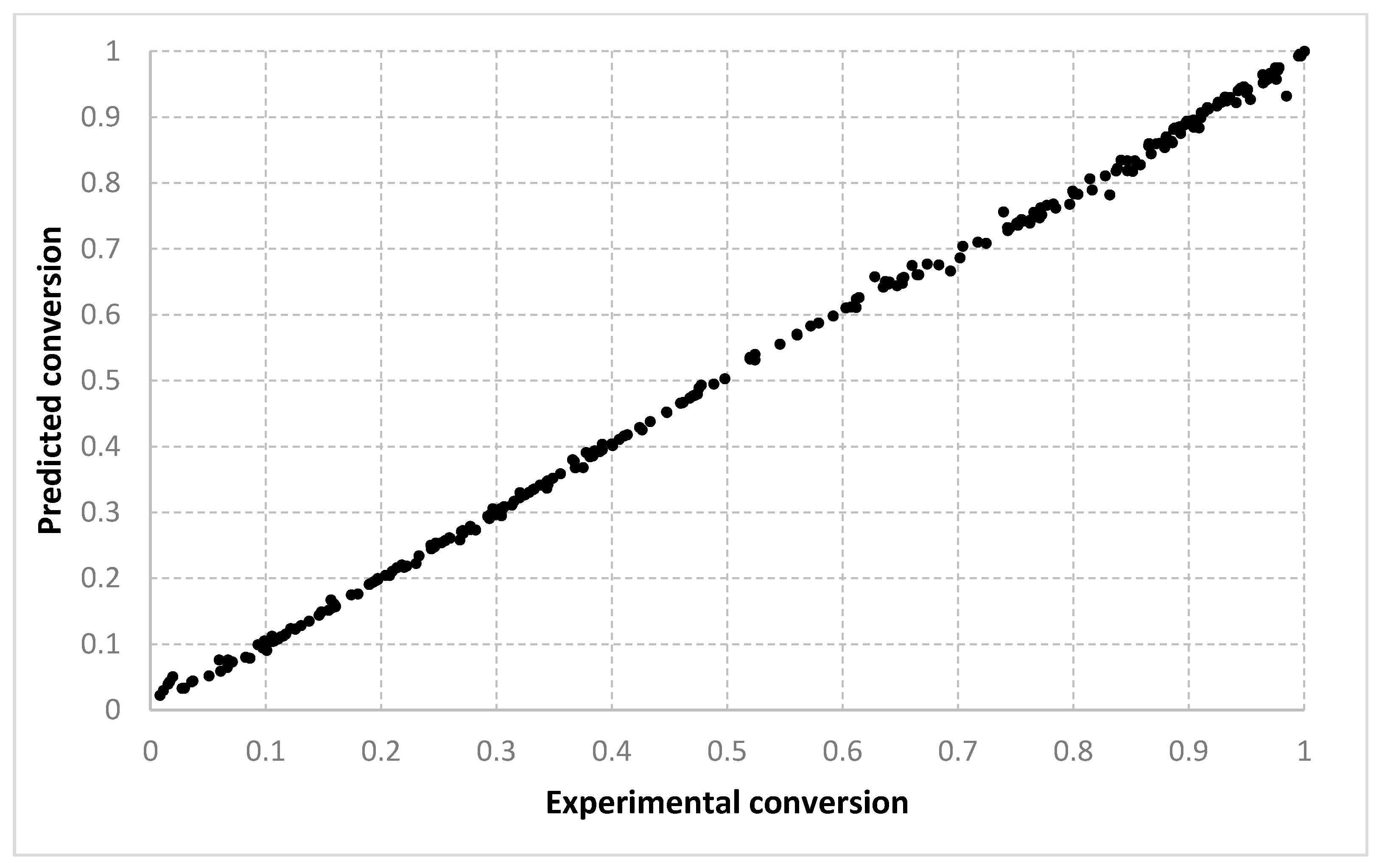
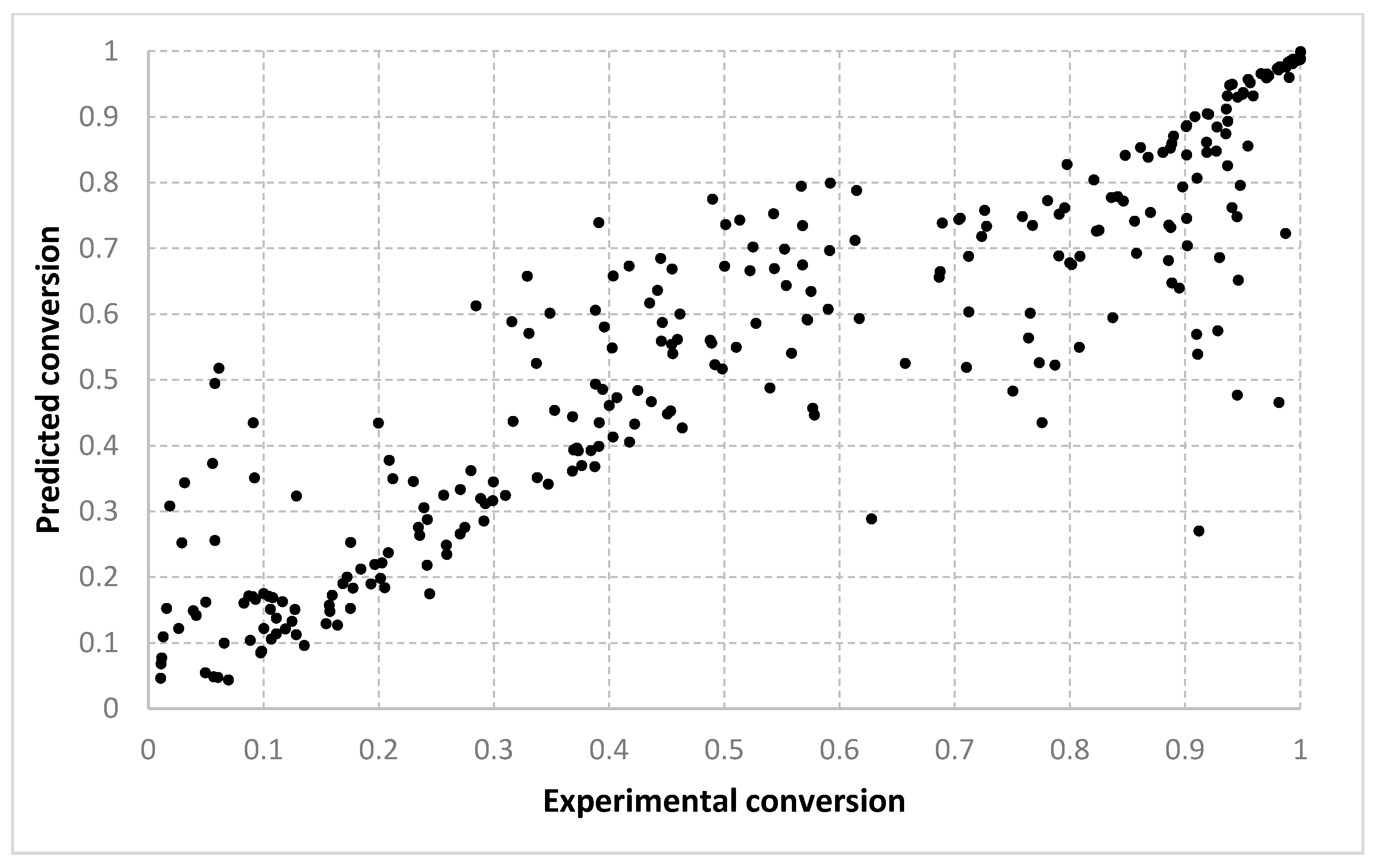
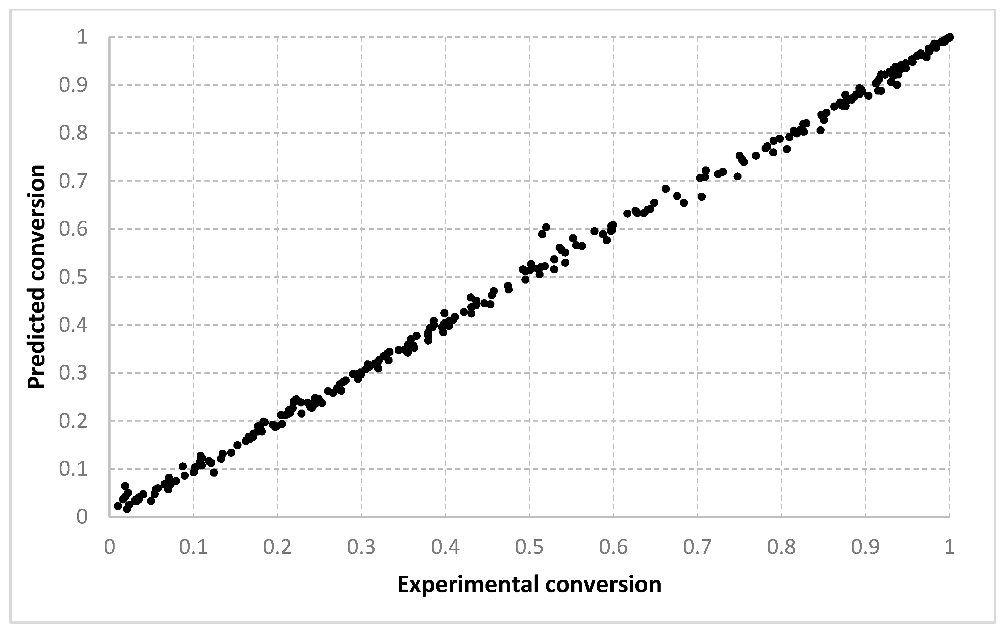
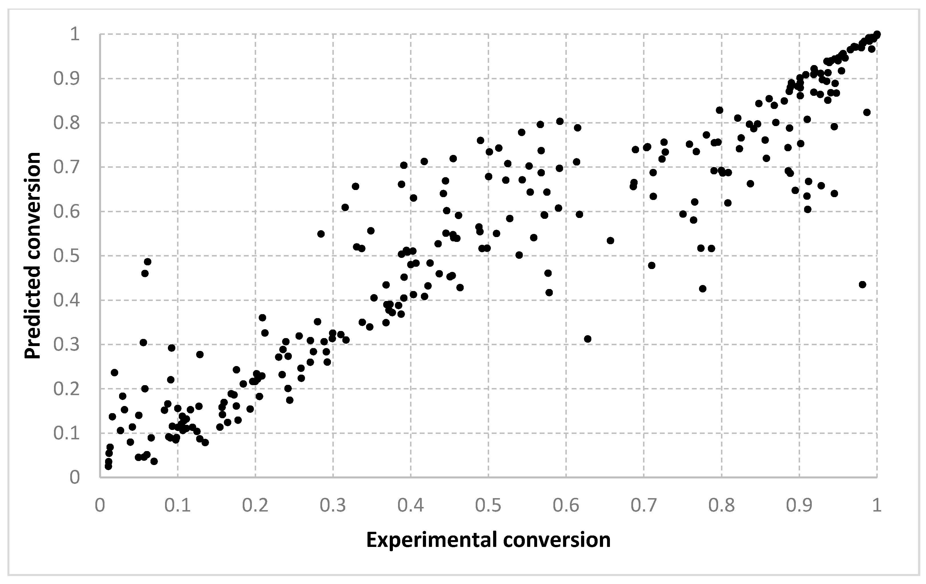
For the conversion, very good results were obtained with all three algorithms, with both types of settings. As shown in Figure 3, Figure 4, Figure 5, Figure 6 and Figure 7, the best fit is obtained with the 90–10% split. With setting 2, slightly better solutions are found. We consider that this is because with two prototypes (i.e., setting 1), the search is being performed in a much larger space. When only one prototype is used (i.e., setting 2), the results are also more continuous. With a 10–90% split, the dispersion of the desired vs. predicted plot is greater. Visually, similar outcomes are achieved for both the LMNNR and RADIAN algorithms. The distribution of the 67–33% split, as seen in Table 3 and Table 4, has an aspect more similar to the 90–10% than to the 10–90% split, with an only slightly larger dispersion. This shows that training with two thirds of the data is enough for good generalization, compared with the extreme case when training only with a tenth of the data (Figure 7 vs. Figure 5).

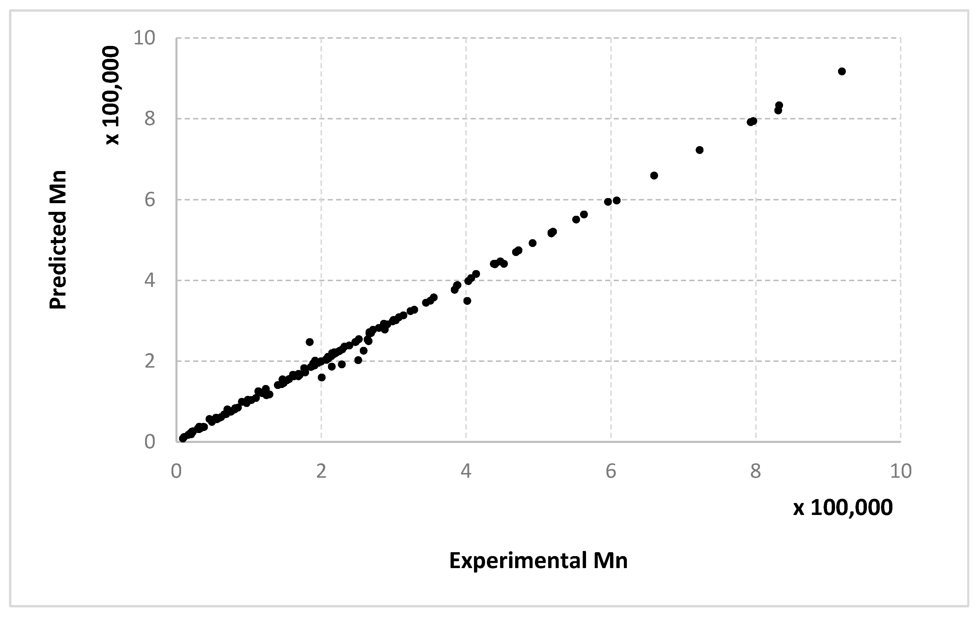
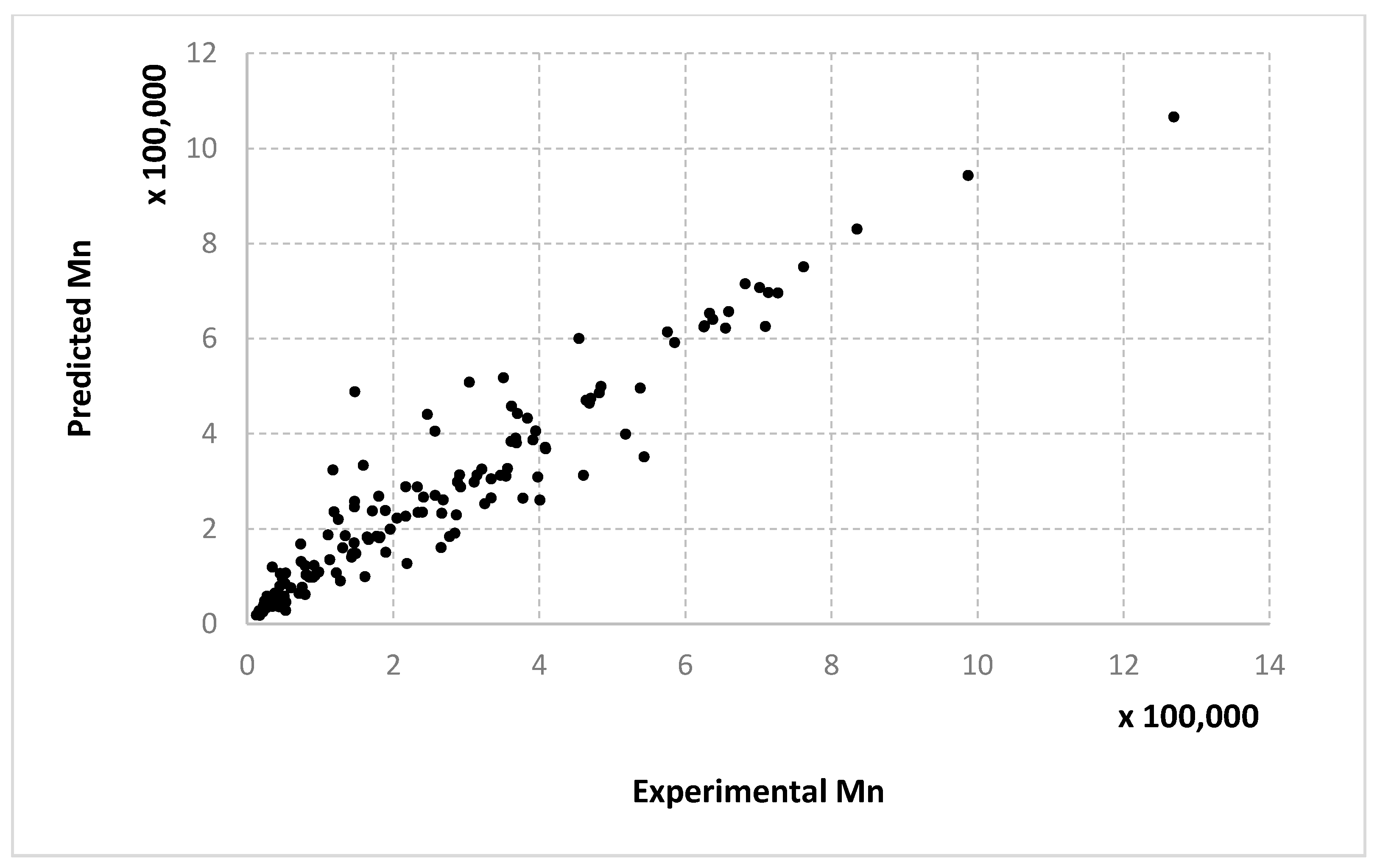
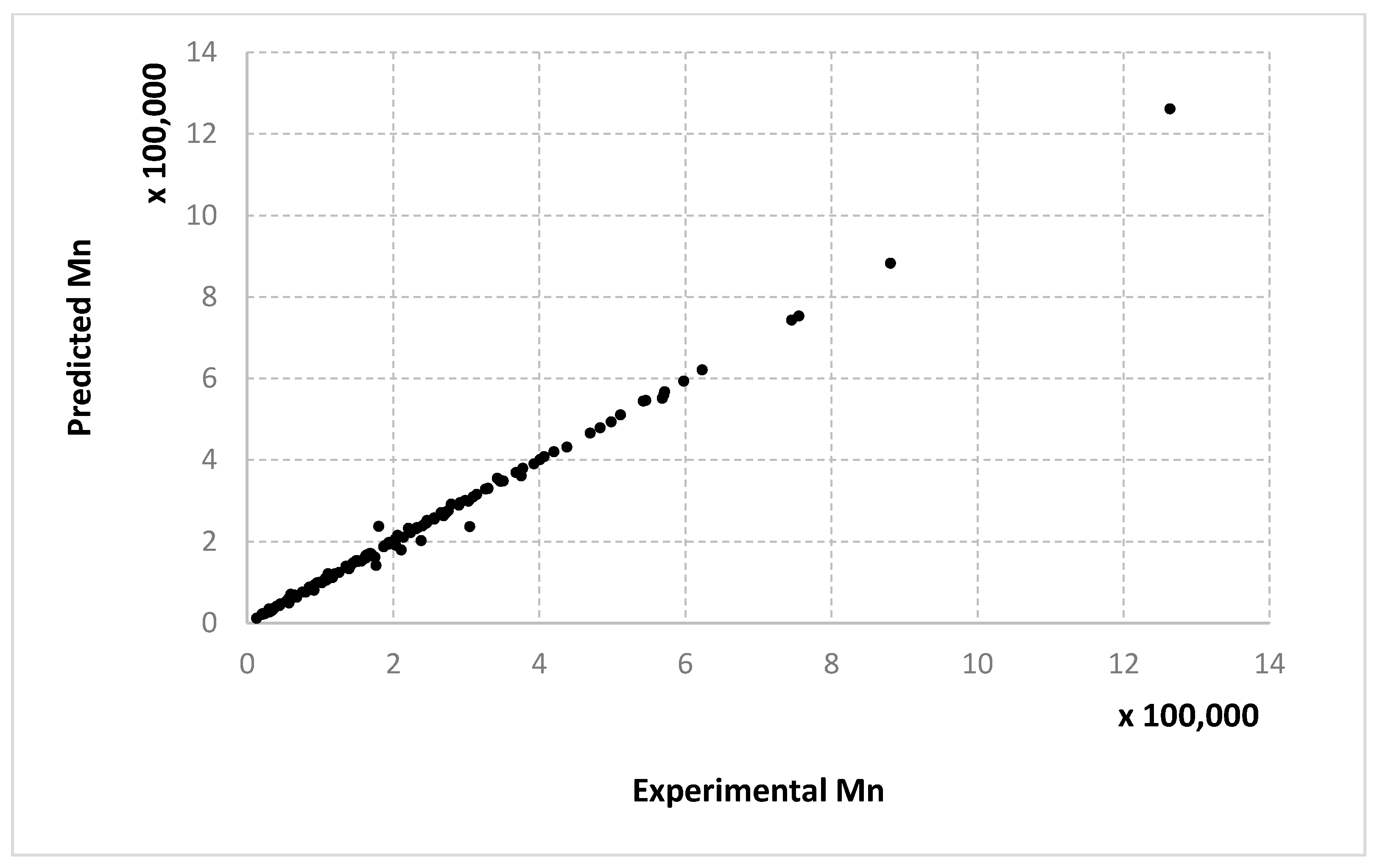
For molecular masses, the conclusions are similar to those obtained for the conversion, with no significant differences between the algorithms. However, one can see here that most of the data in the first half of the domain are much denser than the data from the second half. For M_n, Figure 8, Figure 9 and Figure 10 only display the performance of the RADIAN algorithm (i.e., Algorithm 3). In this case, it is also the data split that has the strongest effect on the results.

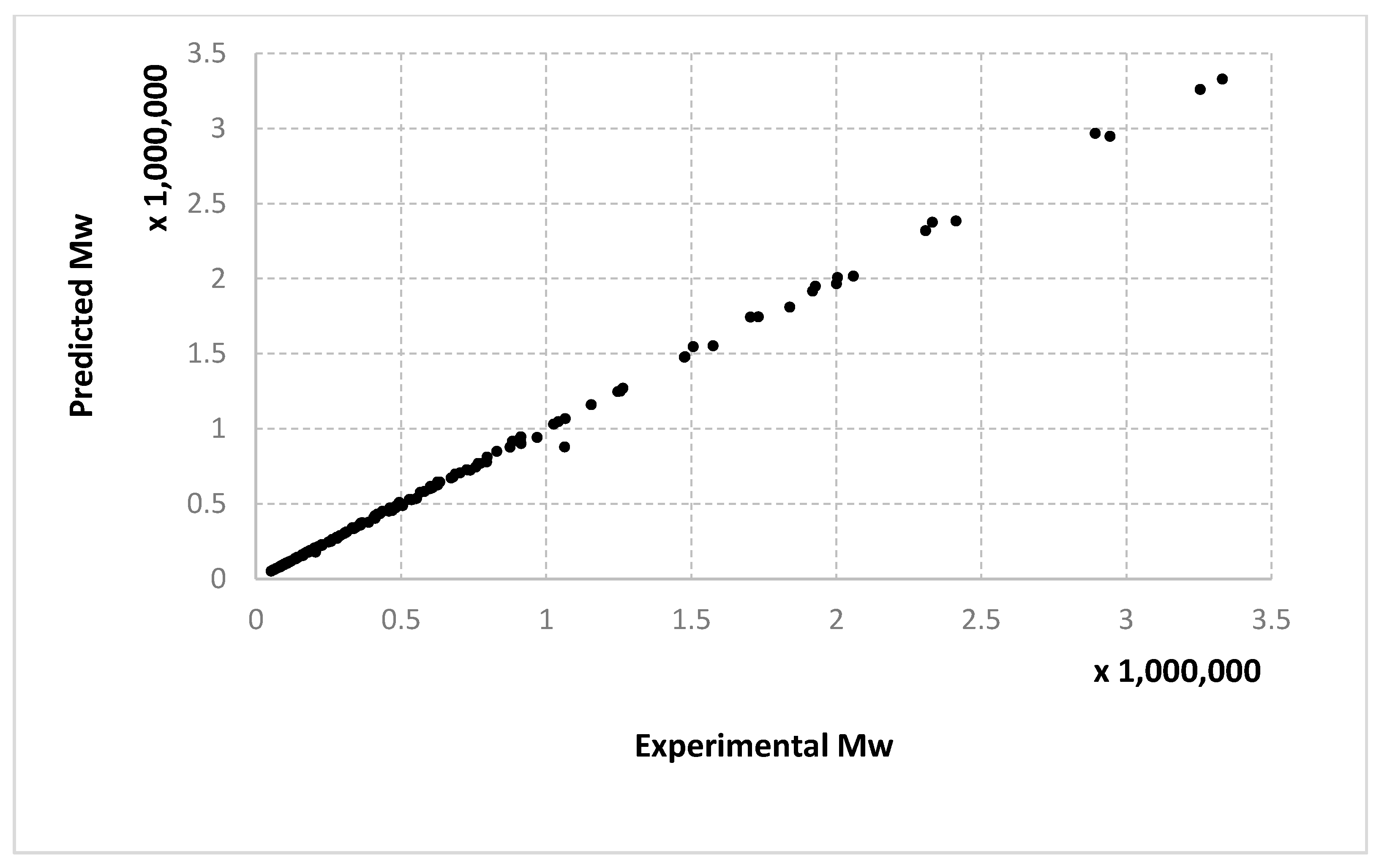
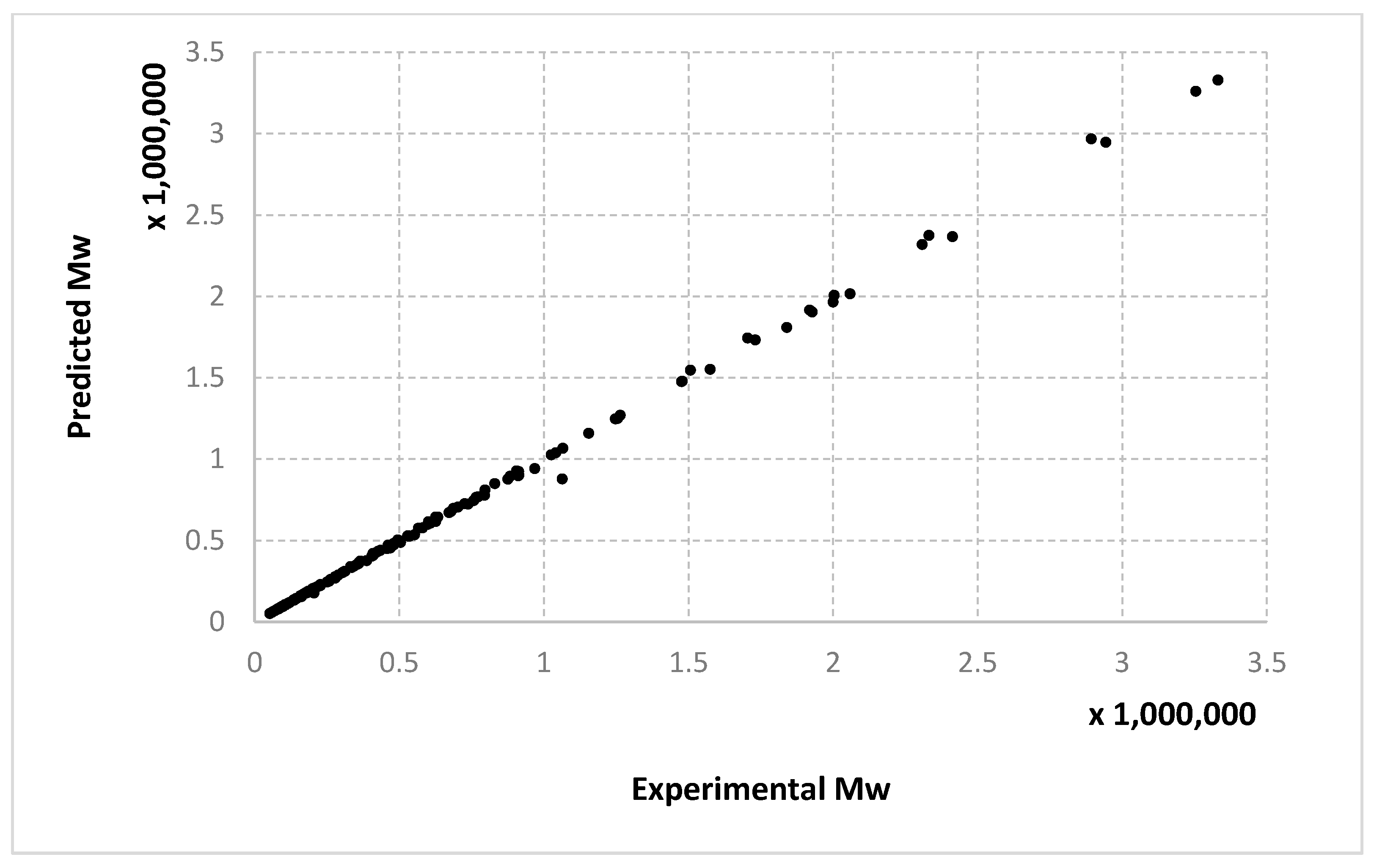
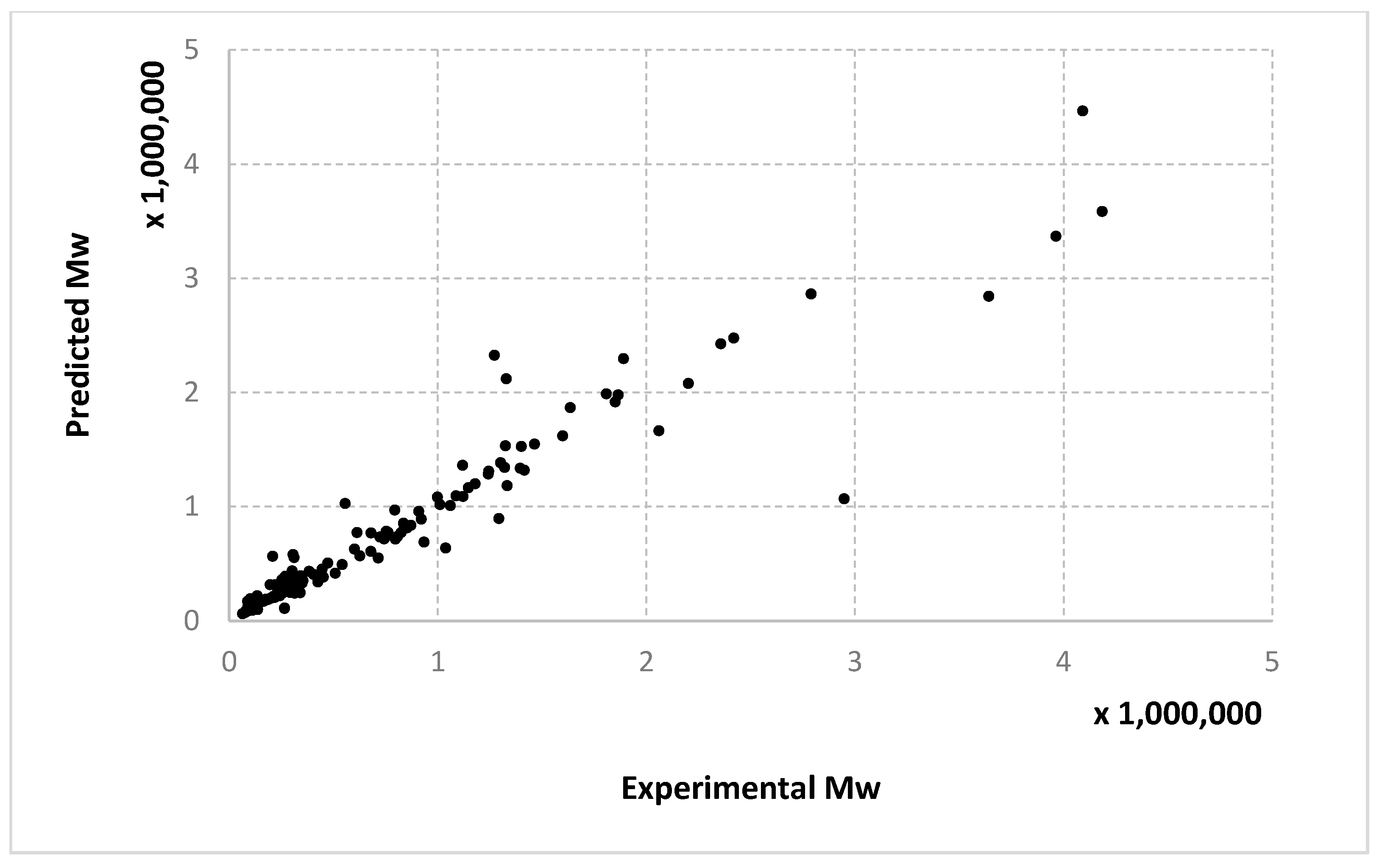
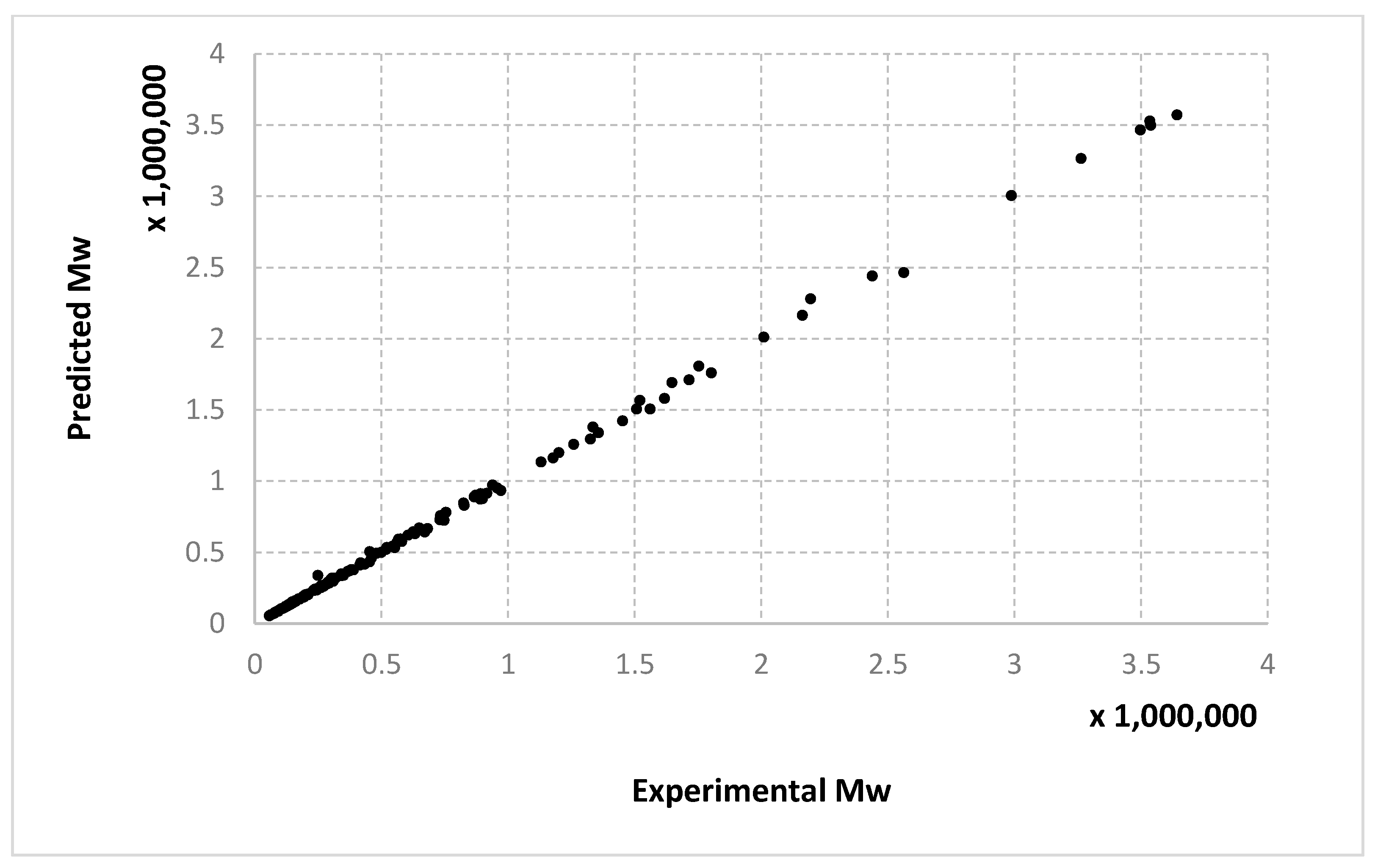
Very similar outcomes are encountered for the M_w output and the LMNNR-EA algorithm (i.e., Algorithm 1). However, in this case, the dispersion of the graph for the 10–90% split is less than those for x an M_n. This is in fact an indicator about the minimum amount of training information needed in order to generalize well.

We remind the reader that the data presented in Figure 3, Figure 4, Figure 5, Figure 6, Figure 7, Figure 8, Figure 9, Figure 10, Figure 11, Figure 12, Figure 13 and Figure 14 refer only to the test data, i.e., the aggregated predictions of the models for the test groups.

The results obtained can also be analyzed in terms of variance of the performance metrics. For all algorithms, the variance decreases when the size of the training set increases. For example, for conversion, in the case of the 10–90% split, the standard deviation σ is about 3–5% of the mean value μ. In the case of the 67–33% split, it becomes 0.1–2% of the mean value and decreases even more for the 90–10% split. The variance can be further decreased by identifying outliers. Since the methods are heuristic, some runs simply fail to provide good solutions. By removing data outside the μ ± 2σ range, the variance is reduced especially for larger training sets, e.g., the new resulting standard deviation is about 10 times smaller. Algorithm 1 has the largest variance among the three methods, while algorithms 2 and 3 have comparable variance.

In terms of execution time, the computations take longer as the size of the training set increases. For example, one fold of cross-validation for conversion takes about 6.7 s for the 10–90% split and 54 s for the 90–10% split for Algorithm 1. Algorithm 2 takes about 5 s and 32 s, respectively. Algorithm 3 requires about 0.7 s and 5.8 s, respectively. These studies were made using a computer with a 4-core 2 GHz Intel processor and 8 GB of RAM. Of course, specific times depend on the particular structure of the training data, especially the number of attributes, and the parameters of the algorithms. In particular, the complexity of Algorithm 1 mainly depends on the number of individuals in the population and the number of generations of the evolutionary algorithm. The complexity of Algorithm 2 mainly depends on the number of iterations of the approximate gradient descent procedure. The complexity of Algorithm 3 mainly depends on the number of hill-climbing steps and the number of neighbors that are generated in each step.

7. Conclusions

Instance-based classification and regression algorithms can provide very good results for complex decision boundaries, especially when the size of the training dataset is big and the number of dimensions of the problem space is not very large. The distance metric is crucial for this class of algorithms, and a significant increase in performance can be achieved by changing it depending on the specific problem under study. The optimal distance metric can be obtained by solving an optimization problem that tries to decrease the distance between the instances with similar output values and increase the distance between the instances with different output values. This process is actually equivalent to maximizing the margin between the instances with different output values. In this way, the concept of a large margin, introduced in the context of support vector machines, can also be applied to instance-based regression. The LMNNR algorithm uses this idea together with prototypes, where each prototype can have its own custom distance metric, which can be helpful when a large number of instances are available.

The corresponding optimization problem can be solved either by an evolutionary algorithm or by an approximate gradient descent method. The results are competitive compared with those obtained by classical algorithms such as support vector machines, k-nearest neighbor and random forest.

Another original regression method is designed by considering an idea from denoising autoencoders, a kind of deep neural networks. In our case, the weights that define the custom distance metric and the positions of the prototypes are computed so as to minimize the mean square error on a corrupted version of the training data created by adding a small amount of noise.

The quality of the results is also supported by the adaptive sampling technique that provides the machine learning algorithms with the most relevant data by taking into account the rate of variation of the outputs involved in the chemical process.

As future directions of research, one may investigate whether similar results can be obtained using alternative techniques, e.g., principal analysis decomposition or (deep) neural networks [9,23,24].

Concerning the case study of the free radical polymerization of MMA, the conclusions that give the necessary practical indications are the following:

• The accuracy of the modeling for the variables of interest—monomer conversion and molecular masses of the polymer—depends on the applied algorithm, the settings of their parameters and the way of splitting the data. The last factor has the greater importance;
• Conversion is easier to model than molecular weights, but, with a proper combination of settings and data sharing, very good results can be obtained for all parameters of interest;
• Although good results have been identified for all three algorithms, RADIAN is preferred because it is considerably faster than the other two, which is an important factor for online optimal control procedures.

References

1. Leon, F.; Curteanu, S. Large Margin Nearest Neighbour Regression Using Different Optimization Techniques. J. Intell. Fuzzy Syst. 2017, 32, 1321–1332. [Google Scholar] [CrossRef]
2. Hall, M.; Frank, E.; Holmes, G.; Pfahringer, B.; Reutemann, P.; Witten, I.H. The WEKA Data Mining Software: An Update. Acm Sigkdd Explor. 2009, 11, 10–18. [Google Scholar] [CrossRef]
3. Leon, F.; Curteanu, S. Evolutionary Algorithm for Large Margin Nearest Neighbour Regression. In Proceedings of the 7th International Conference on Computational Collective Intelligence Technologies and Applications, Madrid, Spain, 21–23 September 2015. [Google Scholar]
4. Leon, F.; Popescu, E. Using Large Margin Nearest Neighbor Regression Algorithm to Predict Student Grades Based on Social Media Traces. In Methodologies and Intelligent Systems for Technology Enhanced Learning; Vittorini, P., Gennari, R., Di Mascio, T., Rodríguez, S., De la Prieta, F., Ramos, C., Silveira, R.A., Eds.; MIS4TEL 2017; Book Series: Advances in Intelligent Systems and Computing; Springer: Cham, Switzerland, 2017; Volume 617. [Google Scholar]
5. Popescu, E.; Leon, F. Predicting Academic Performance Based on Learner Traces in a Social Learning Environment. IEEE Access 2018, 6, 72774–72785. [Google Scholar] [CrossRef]
6. Leon, F.; Piuleac, C.G.; Curteanu, S.; Poulios, I. Instance-based regression with missing data applied to a photocatalitic oxidation process. Cent. Eur. J. Chem. 2012, 10, 1149–1156. [Google Scholar]
7. Mareci, D.; Sutiman, D.; Chelariu, R.; Leon, F.; Curteanu, S. Evaluation of the corrosion resistance of new TiZr binary alloys by experiment and simulation based on regression model with incomplete data. Corros. Sci. 2013, 73, 106–122. [Google Scholar] [CrossRef]
8. Curteanu, S.; Leon, F.; Lupu, A.S.; Floria, S.A.; Logofatu, D. An Evaluation of Regression Algorithms Performance for the Chemical Process of Naphthalene Sublimation. In Proceedings of the 14th International Conference on Artificial Intelligence Applications and Innovations (AIAI 2018), Rhodes, Greece, 25–27 May 2018; Volume 519, pp. 219–230. [Google Scholar]
9. Goodfellow, I.; Bengio, Y.; Courville, A. Deep Learning; MIT Press: Cambridge, MA, USA, 2016. [Google Scholar]
10. Chiu, W.Y.; Carratt, G.M.; Soong, D.S. A computer model for the gel effect in free-radical polymerization. Macromolecules 1983, 16, 348–359. [Google Scholar] [CrossRef]
11. Curteanu, S.; Bulacovschi, V.; Lisa, C. Algorithms for using some models of gel and glass effects in free-radical polymerization of methyl methacrylate. Polym. Plast. Technol. Eng. 1999, 38, 1121–1136. [Google Scholar] [CrossRef]
12. Curteanu, S.; Leon, F.; Gâlea, D. Neural network models for free radical polymerization of methyl methacrylate. Eurasian Chem. Technol. J. 2003, 5, 225–231. [Google Scholar]
13. Curteanu, S. Direct and inverse neural network modeling in free radical polymerization. Cent. Eur. J. Chem. 2004, 2, 113–140. [Google Scholar] [CrossRef]
14. Curteanu, S.; Leon, F. Hybrid neural network models applied to a free radical polymerization process. Polym. Plast. Technol. Eng. 2006, 45, 1013–1023. [Google Scholar] [CrossRef]
15. Tian, Y.; Zhang, J.; Morris, J. Modeling and Optimal Control of a Batch Polymerization Reactor Using a Hybrid Stacked Recurrent Neural Network Model. Ind. Eng. Chem. Res. 2001, 40, 4525–4535. [Google Scholar] [CrossRef]
16. Shepard, R.N. Psychological representations of speech sounds. In Human Communication: A Unified View; David, E.E., Denes, P.B., Eds.; McGraw-Hill: New York, NY, USA, 1972. [Google Scholar]
17. Rumelhart, D.E.; Abrahamsen, A.A. A model for analogical reasoning. Cognit. Psychol. 1973, 5, 1–28. [Google Scholar] [CrossRef]
18. Weinberger, K.Q.; Saul, L.K. Distance metric learning for large margin nearest neighbor classification. J. Mach. Learn. Res. 2009, 10, 207–244. [Google Scholar]
19. Kumar, M.P.; Torr, P.H.S.; Zisserman, A. An Invariant Large Margin Nearest Neighbour Classifier. In Proceedings of the IEEE 11th International Conference on Computer Vision (ICCV 2007), Rio de Janeiro, Brazil, 14–21 October 2007. [Google Scholar] [CrossRef]
20. Assi, K.C.; Labelle, H.; Cheriet, F. Modified large margin nearest neighbor metric learning for regression. IEEE Signal Process. Lett. 2014, 21, 292–296. [Google Scholar] [CrossRef] [Green Version]
21. Curteanu, S.; Bulacovschi, V.; Constantinescu, M. Free radical polymerization of methyl methacrylate. Modelling and simulation at high conversion. Hung. J. Ind. Chem. 1999, 27, 287–292. [Google Scholar]
22. Leon, F.; Curteanu, S. Performance Comparison of Different Regression Methods for a Polymerization Process with Adaptive Sampling. In Proceedings of the 18th International Conference on Computational Intelligence and Systems Sciences, Prague, Czechia, 18–22 November 2016. [Google Scholar]
23. Mercorelli, P. Biorthogonal wavelet trees in the classification of embedded signal classes for intelligent sensors using machine learning applications. J. Frankl. Inst. 2007, 344, 813–829. [Google Scholar] [CrossRef]
24. Mercorelli, P. Denoising and harmonic detection using nonorthogonal wavelet packets in industrial applications. J. Syst. Sci. Complex. 2007, 20, 325–343. [Google Scholar] [CrossRef]
Figure 1. Adaptively sampled points (337) for the monomer conversion (x).
Mathematics 09 00547 g001
Figure 2. Adaptively sampled points (414) for the numerical average molecular weight (Mn).
Mathematics 09 00547 g002
Figure 3. Predicted conversion with the LMNNR-EA algorithm versus experimental conversion, setting 1, with data split into 90% for training and 10% for testing.
Mathematics 09 00547 g003
Figure 4. Predicted conversion with the RADIAN algorithm versus experimental conversion, setting 2, with data split into 90% for training and 10% for testing.
Mathematics 09 00547 g004
Figure 5. Predicted conversion with the LMNNR-AGD algorithm versus experimental conversion, setting 2, with data split into 10% for training and 90% for testing.
Mathematics 09 00547 g005
Figure 6. Predicted conversion with the RADIAN algorithm versus experimental conversion, setting 1, with data split into 10% for training and 90% for testing.
Mathematics 09 00547 g006
Figure 7. Predicted conversion with the LMNNR-AGD algorithm versus experimental conversion, setting 2, with data split into 67% for training and 33% for testing.
Mathematics 09 00547 g007
Figure 8. Predicted numerical average molecular weight with the RADIAN algorithm versus experimental data, setting 1, with data split into 90% for training and 10% for testing.
Mathematics 09 00547 g008
Figure 9. Predicted numerical average molecular weight with the RADIAN algorithm versus experimental data, setting 2, with data split into 10% for training and 90% for testing.
Mathematics 09 00547 g009
Figure 10. Predicted numerical average molecular weight with the RADIAN algorithm versus experimental data, setting 2, with data split into 67% for training and 33% for testing.
Mathematics 09 00547 g010
Figure 11. Predicted gravimetrical average molecular weight with the LMNNR-EA algorithm versus experimental data, setting 1, with data split into 90% for training and 10% for testing.
Mathematics 09 00547 g011
Figure 12. Predicted gravimetrical average molecular weight with the LMNNR-EA algorithm versus experimental data, setting 2, with data split into 90% for training and 10% for testing.
Mathematics 09 00547 g012
Figure 13. Predicted gravimetrical average molecular weight with the LMNNR-EA algorithm versus experimental data, setting 2, with data split into 10% for training and 90% for testing.
Mathematics 09 00547 g013
Figure 14. Predicted gravimetrical average molecular weight with the LMNNR-EA algorithm versus experimental data, setting 2, with data split into 67% for training and 33% for testing.
Mathematics 09 00547 g014