On the Application of the Generalized Means to Construct Multiresolution Schemes Satisfying Certain Inequalities Proving Stability

Abstract

Multiresolution representations of data are known to be powerful tools in data analysis and processing, and they are particularly interesting for data compression. In order to obtain a proper definition of the edges, a good option is to use nonlinear reconstructions. These nonlinear reconstruction are the heart of the prediction processes which appear in the definition of the nonlinear subdivision and multiresolution schemes. We define and study some nonlinear reconstructions based on the use of nonlinear means, more in concrete the so-called Generalized means. These means have two interesting properties that will allow us to get associated reconstruction operators adapted to the presence of discontinuities, and having the maximum possible order of approximation in smooth areas. Once we have these nonlinear reconstruction operators defined, we can build the related nonlinear subdivision and multiresolution schemes and prove more accurate inequalities regarding the contractivity of the scheme for the first differences and in turn the results about stability. In this paper, we also define a new nonlinear two-dimensional multiresolution scheme as non-separable, i.e., not based on tensor product. We then present the study of the stability issues for the scheme and numerical experiments reinforcing the proven theoretical results and showing the usefulness of the algorithm.

1. Introduction

Multiresolution representations are one of the most efficient tools for data compression, and in particular for image compression. The multi-scale representation of a signal is well adapted to quantization or simple thresholding.

We start the algorithm with an input data $f^L,$ obtaining a multiresolution version of the initial data, which is processed according to the desired application in mind. After decoding the processed representation, we obtain a discrete set ${\widehat{f}}^L$ which is expected to be close to the original discrete set $f^L$. In order for this to be true, some form of stability is needed, i.e., we must require that

$$||{\widehat{f}}^L-f^L||\le \sigma ({ϵ}_0,{ϵ}_1,\dots ,{ϵ}_L),$$

where $\sigma (·,\dots ,·)$ satisfies

$$\underset{{ϵ}_l\to 0,0\le l\le L}{lim}\sigma ({ϵ}_0,{ϵ}_1,\dots ,{ϵ}_L)=0.$$

Harten’s framework for multiresolution provides an adequate setting for the design of discrete multiresolution representations [1]. Discrete resolution levels are connected by inter-resolution operators, named decimation (from fine $(k)$ to coarse $(k-1)$) and prediction (from coarse to fine). These inter-scale operators are directly related to the discretization and reconstruction operators, which act between the continuous level (where a function f, related to the discrete data, lives) to each discrete level (where $f^k$ lives). The greatest advantage of Harten’s general framework lies in its adaptability. The fundamental role played by the reconstruction operator makes it possible to perform specific adaptive treatments at singularities. In general, this involves data-dependent reconstruction operators, which lead to nonlinear prediction schemes and, hence, to nonlinear multiresolution decompositions [1].

Linear multiresolution schemes derived following Harten’s framework can be also recovered from the theory of wavelets. Many applications have been found for this kind of algorithms; see, for example, References [2,3]. Nonlinearity in these contexts can bring some improvements when discontinuities are presented in the data.

Some nonlinear multiresolution schemes have been previously studied and they have been the starting point to the improvement that we propose in this paper. In particular, we refer to the PPH nonlinear multiresolution scheme presented in References [4,5,6], which gives quite nice visual effects in the reconstructions. This scheme is proven to be stable in $1D$ (see Reference [7]), but nothing is proven for higher dimensions. A possibility to find nonlinear stable two-dimensional multiresolution schemes is to considered the non-separable approach introduced in Reference [8]. But a good candidate for the prediction operator with the right contraction properties was still to be found. In this paper, we present subdivision and multiresolution schemes based on the use of the so-called generalized means, which give rise to more accurate contractivity constants according to a crucial inequality for the first differences of the proposed schemes. This fact allows us to easily prove more accurate stability results as much in $1D$ as in $2D.$ We know some references where the generalized means have been previously used in different practical applications with interesting results; see, for example, References [9,10].

Since nonlinearity seems to be crucial to get more accurate results, it is also important to point out the promising role that could play artificial intelligence in order to design adapted algorithms with optimal properties; see, for example, Reference [11], for papers on this matter.

The paper is organized as follows: In Section 2, we recall the basic concepts of point value multiresolution in 2D. In particular, we give the two-dimensional non-separable multiresolution algorithms to be used. In Section 3, we define and study the new particular prediction operators based on the generalized means and prove important properties. In Section 4, we present the stability results giving the main inequality ensuring stability. Some numerical experiments are given in Section 5. Finally, in Section 6, we present some conclusions and future perspectives.

2. Harten Multiresolution in 2D

We introduce in this section the basic concepts about multiresolution that we will need for the rest of the paper. In particular, we will be working mainly in the point value setting. We refer to the interested reader to Reference [12] for a more detailed description about multiresolution.

Let us consider the grid in ${[0,1]}^2$ given by

$$X^l={\{x_{i_1}^l,x_{i_2}^l\}}_{i_1,i_2=0}^{J_l},J_l=2^l{J}_0,J_0\mathrm{integer},h_l=\frac{1}{J_0{2}^l},$$

and the discretization operator for point values

$${\mathcal{D}}_l:\left\{\begin{array}{cc}C({[0,1]}^2)\hfill & \to V^l\hfill \\ f\hfill & \mapsto f^l={(f_{i_1,i_2}^l)}_{i_1,i_2=1}^{J_l},\hfill \end{array}\right.$$

(1)

where $f_{i_1,i_2}^l,0\le i_s\le J_l,s=1,2$ is defined by

$$f_{i_1,i_2}^l:=f(x_{i_1},x_{i_2}).$$

(2)

$C({[0,1]}^2)$ is the space of continuous functions in ${[0,1]}^2$, and $V^l$ is the space of real sequences of dimension ${(J_l+1)}^2$ related with the resolution of $X^l$.

An associated reconstruction operator ${\mathcal{R}}_l$ for this discretization is any right inverse of ${\mathcal{D}}_l$, which means that, for all $f^l\in V^l$, ${\mathcal{R}}_l{f}^l\in C({[0,1]}^2)$ and

$$f_{i_1,i_2}^l=({\mathcal{R}}_l{f}^l)(x_{i_1},x_{i_2}).$$

(3)

Thus, for the point value setting, the reconstruction operator amounts to an interpolation.

The sequences $\left\{{\mathcal{D}}_l\right\}$ and $\left\{{\mathcal{R}}_l\right\}$ define a multiresolution transform, and the prediction operator, $P_{l-1}^l:={\mathcal{D}}_{l+1}{\mathcal{R}}_l:V^l\to V^{l+1}$, defines an associated subdivision scheme. If ${\mathcal{R}}_l$ is a nonlinear operator, then the corresponding subdivision and multiresolution schemes are also nonlinear.

The decimation operator $D_l^{l-1}:V^l\to V^{l-1}$ is always linear and, in our case, can be expressed as

$$f_{i_1,i_2}^{l-1}={(D_l^{l-1}{f}^l)}_{i_1,i_2}={({\mathcal{D}}_{l-1}{\mathcal{R}}_l{f}^l)}_{i_1,i_2}=f_{2i_1,2i_2}^l.$$

(4)

We also need to define the errors that, in this case, are given by

$$e_{j_1,j_2}^l:=f_{j_1,j_2}^l-{(P_{l-1}^l{f}^{l-1})}_{j_1,j_2}.$$

(5)

It is easy to prove that the errors belong to the null space of the decimation operator; in fact,

$$D_l^{l-1}{e}_{2i_1,2i_2}^l=D_l^{l-1}(f_{2i_1,2i_2}^l-{(P_{l-1}^l{f}^{l-1})}_{2i_1,2i_2})=f_{i_1,i_2}^{l-1}-D_l^{l-1}{(P_{l-1}^l{f}^{l-1})}_{2i_1,2i_2};$$

(6)

therefore, taking into account that the prediction operator inherits the consistency property from the reconstruction operator, i.e., it is a right inverse of the decimation operator, we have

$$e_{2i_1,2i_2}^l=0,$$

(7)

which, in practice, means that there is redundancy in the errors, and it is sufficient to keep the errors which are located at a position with any odd coordinate.

We now have all the needed ingredients to give the coding and decoding multiresolution algorithms. Let us denote first:

$$\begin{array}{ccc}\hfill J:& =& \{(j_1,j_2):j_s\in \{2i_s-1,2i_s\},s=1,2\},\hfill \\ \hfill J^{\prime }:& =& J\backslash \{j_1=2i_1,j_2=2i_2\}.\hfill \end{array}$$

Then, the mentioned algorithms take the form:

These algorithms, Algorithms 1 and 2, are nothing more than another representation of the initial data, which is better adapted to processes of compression and denoising. These processes will be done to the multiresolution representation of the data $\mu (f^L)$ before the decompression stage. Notice that the better the nonlinear prediction the larger the attained compression after simple truncation, since many details would be close to zero. We would also like to emphasize a strategy that allows Algorithms 1 and 2 to control the rate of compression, just keeping the chosen percentage of the kept details in the multiresolution representation, setting to zero the rest of them. If, on the contrary, one wants to monitor the total accumulated error that will be expected after pre-processing the multiresolution of the data and applying the decoding algorithm, then, one needs to consider Algorithm 3, which includes some slight modifications according to the theoretical result in Theorem 1.

Algorithm 1: $\mu (f^L)=M{f}^L$  (Coding)

for l = L,…,1

for i1, i2 = 0,…, Jl−1

$f_{i_1,i_2}^{l-1}=f_{{2i}_1,{2i}_2}^l$

for $(j_1,j_2)\in J^{\prime }$

$e_{j_1,j_2}^l=f_{j_1,j_2}^l-{(P_{l-1}^l{f}^{l-1})}_{j_1,j_2}$

end

end

end

Algorithm 2: $f^L=M^{-1}\mu (f^L)$  (Decoding)

for l = L,…,1

for i1, i2 = 0,…, Jl−1

for $(j_1,j_2)\in J^{\prime }$

$f_{j_1,j_2}^l={(P_{l-1}^l{f}^{l-1})}_{j_1,j_2}+e_{j_1,j_2}^l$

end

$f_{2i_1,2i_2}^l=f_{i_1,i_2}^{l-1}$

end

end

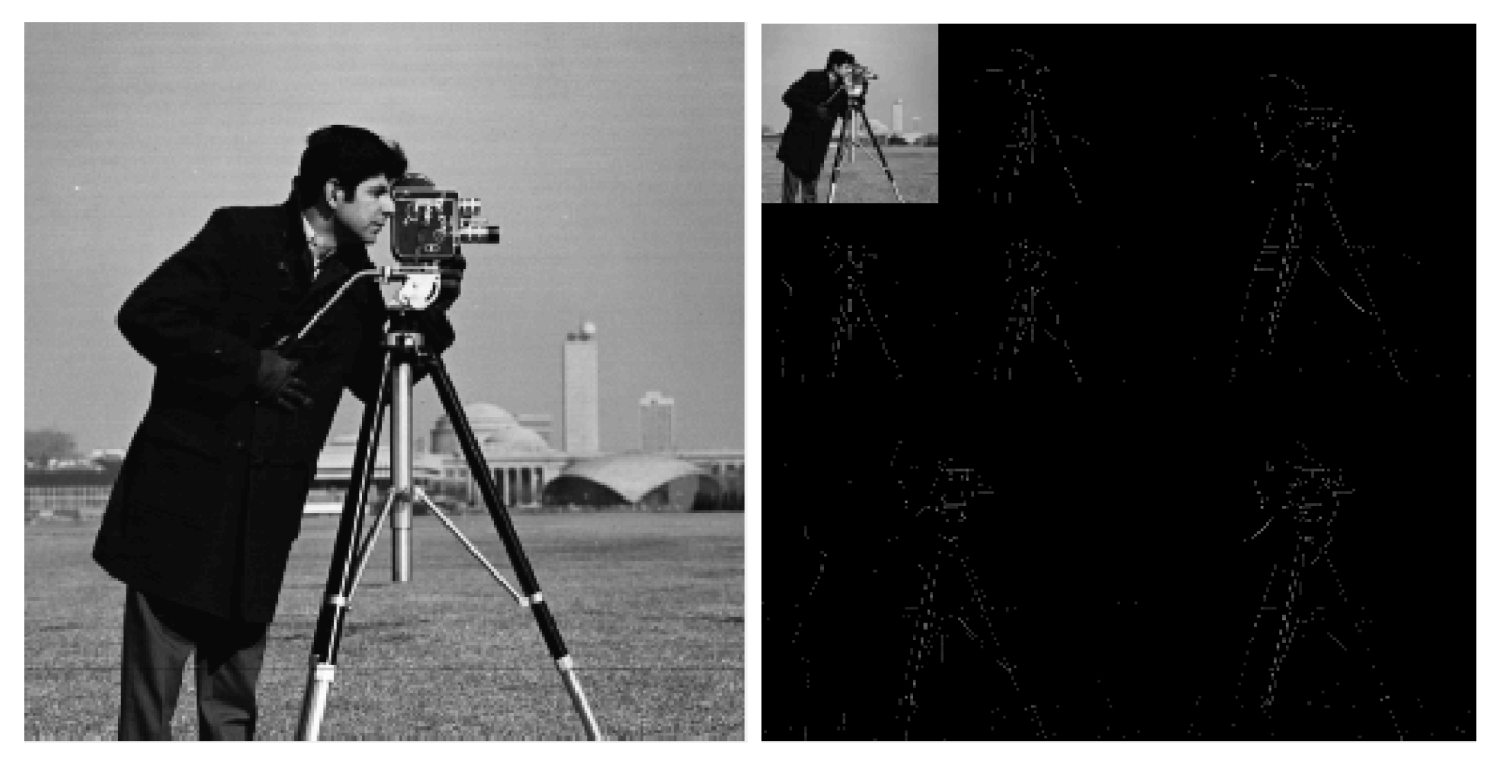
Algorithm 1 starts descending one scale from the original data and then reorganizes the coefficient matrix at each step in order to continue working with the significant coefficients of the multiresolution representation to compute another scale. In Figure 1, we show a related application in image processing of the cell average version of Algorithm 1, in which it is easy to observe the scales and the different types of coefficients. In Figure 1, to the right we see two scales of the multiresolution version of the data. In the upper left corner, one can see the second step of Algorithm 1 for $L=2$ applied to the significative coefficients resulting after the first step for $L=1.$ In the upper right, bottom left, and bottom right corners appear the detail coefficients, which, in some cases, are below a given tolerance and have been set to zero (this is why they appear in black color.)

Algorithm 3: $\tilde{\mu }(f^L)=\tilde{M}{f}^L$  (Alternative Coding to monitor the accumulated error)

Given $ϵ$

$\delta =\frac{ϵ}{\tilde{C}L}$

for l = L,…,1

for i1, i2 = 0,…, Jl−1

$f_{i_1,i_2}^{l-1}=f_{{2i}_1,{2i}_2}^l$

for $(j_1,j_2)\in J^{\prime }$

Compute ${(P_{l-1}^l{f}^{l-1})}_{j_1,j_2}$ using (9) and choosing the case

according to the index $(j_1,j_2)$

$e_{j_1,j_2}^l=f_{j_1,j_2}^l-{(P_{l-1}^l{f}^{l-1})}_{j_1,j_2}$

end

end

${\tilde{e}}^l=tr(e^l,\delta )$

end

$\tilde{\mu }(f^L)=\{f^0,{\tilde{e}}^1,\dots ,{\tilde{e}}^L\}.$

3. A Prediction Operator Based on the Generalized Means

Our objective in this section is the definition of an adapted nonlinear prediction operator with desirable properties regarding to adaption to potential discontinuities, order of approximation, and stability issues of the associated subdivision and multiresolution schemes.

First, we define the generalized means, which appear in the definition of the new prediction operator. The generalized means depending on $m\in \mathbb{Z}$ of n positive values $x_1,x_2,\dots ,x_n$ are given by

$$G{M}_m(x_1,x_2,\dots ,x_n):=\left\{\begin{array}{cc}{\left(x_1{x}_2\cdots x_n\right)}^{\frac{1}{n}}\hfill & m=0\hfill \\ {\left({\displaystyle \frac{1}{n}\sum _{i=1}^n{x}_i^m}\right)}^{\frac{1}{m}}\hfill & m\ne 0.\hfill \end{array}\right.$$

We are interested in the case $n=2,$ since we will be working in $2D$ with fourth order reconstructions, and in the value of the parameter $m=-k,k\in \mathbb{N}\backslash \left\{0\right\}.$ Therefore, the considered means read

$$G{M}_k(x_1,x_2):={(\frac{2x_1^k{x}_2^k}{x_1^k+x_2^k})}^{\frac{1}{k}}.$$

Notice that, in order to apply the $G{M}_k$ mean in the definition of the prediction operator, we need to redefine it in ${\mathbb{R}}^2$ in the following way:

$$G{M}_k(x,y):=\left\{\begin{array}{cc}sgn(x){(\frac{2x^k{y}^k}{x^k+y^k})}^{\frac{1}{k}}\hfill & \mathrm{if}xy>0,\hfill \\ 0\hfill & \mathrm{otherwise},\hfill \end{array}\right.$$

(8)

where $sgn(x)$ stands for the sign of $x.$

Some of the basic properties of these means appear in the following lemma,

Lemma 1.

For any couples$(x,y)$,$(x^{\prime },y^{\prime })\in {\mathbb{R}}_{+}^2$, the function$G{M}_k$, with$k\in \mathbb{N}\backslash \left\{0\right\}$satisfies the following properties:

• $G{M}_i(x,y)\le G{M}_j(x,y)$, if $i\le j$.
• $GM(k)=G{M}_k(x,y)$, is continuous in k.
• $G{M}_k(x,y)=G{M}_k(y,x).$
• $G{M}_k(-x,-y)=-G{M}_k(x,y).$
• $G{M}_k(x,y)=0,$ if $xy\le 0.$
• $min\{|x|,|y|\}\le |G{M}_k(x,y)|\le max\{|x|,|y|\}.$

We refer to three more properties of these means that will be useful later to attain adaption in case of discontinuities, order of approximation in smooth areas, and stability results, respectively.

Lemma 2.

(Adaption to discontinuities) For any couple $(x,y)\in {\mathbb{R}}_{+}^2$, i.e., $x>0$, $y>0,$

$$|G{M}_k(x,y)|\le \sqrt[k]{2}min\{|x|,|y|\}.$$

Proof. 

Without lost of generality, we consider $x<y$:

$$\begin{array}{ccc}G{M}_k(x,y)\hfill & =& {\displaystyle \sqrt[k]{\frac{2x^k{y}^k}{x^k+y^k}}=x\sqrt[k]{\frac{2y^k}{x^k+y^k}}}\hfill \\ & \le & {\displaystyle \sqrt[k]{2}\sqrt[k]{\frac{y^k}{x^k+y^k}}x\le \sqrt[k]{2}min\{x,y\}.}\hfill \end{array}$$

□

Lemma 3.

(Order of approximation) For any couple $(x,y)\in {\mathbb{R}}_{+}^2$, i.e., $x>0$, $y>0,$ satisfying $x=O(1)$, $y=O(1)$, and $|x-y|=O(h)$, then

$$|G{M}_k(x,y)-\frac{x+y}{2}| =O(h^2).$$

Proof. 

In order to get this result, it will be useful to rewrite the $G{M}_k$ means as

$$G{M}_k(x,y):={(\frac{2x^k{y}^k}{x^k+y^k})}^{\frac{1}{k}}= (\frac{x^k+y^k}{2}){(1-{(\frac{x^k-y^k}{x^k+y^k})}^2)}^{\frac{1}{k}}.$$

Then, our proof is based on the following observations:

(a)

$$|\frac{2x^k{y}^k}{x^k+y^k}-\frac{x^k+y^k}{2}| =O(h^2).$$

(b)

If $A>0$, $B>0$, satisfy $|A-B|=O(h^2)$, then

$$|A^{\frac{1}{k}}-B^{\frac{1}{k}}| =O(h^2),$$

(c)

$$|\frac{x^k+y^k}{2}-{(\frac{x+y}{2})}^k| =O(h^2).$$

The proof of the first observation comes from the fact that

$$\frac{2x^k{y}^k}{x^k+y^k}=\frac{x^k+y^k}{2}(1-{(\frac{x^k-y^k}{x^k+y^k})}^2);$$

hence,

$$|\frac{2x^k{y}^k}{x^k+y^k}-\frac{x^k+y^k}{2}| =|-\frac{x^k+y^k}{2}{(\frac{(x-y)(x^{k-1}+x^{k-2}y+\dots +y^{k-1})}{x^k+y^k})}^2| =O(h^2).$$

For the second observation, we simply apply the basic Lagrange theorem to the function $f(x)=x^{\frac{1}{k}};$ thus,

$$|A^{\frac{1}{k}}-B^{\frac{1}{k}}| = |\frac{1}{k}{c}^{\frac{1}{k}-1}(A-B)|=O(h^2),$$

with c an intermediate point between A and $B,$ and then $c=O(1)$.

Finally, to prove the third observation, we use the following developments using the Newton binomial theorem,

$$\begin{array}{ccc}\hfill {(\frac{x+y}{2})}^k& =& {\displaystyle \frac{1}{2^k}(\sum _{j=0}^k\left(\genfrac{}{}{0pt}{}{k}{j}\right)x^j{y}^{k-j}),}\hfill \\ \hfill \frac{x^k+y^k}{2}& =& \frac{1}{2^k}({(1+1)}^{k-1}{x}^k+{(1+1)}^{k-1}{y}^k)\hfill \\ & =& {\displaystyle \frac{1}{2^k}(\sum _{j=0}^{k-1}\left(\genfrac{}{}{0pt}{}{k-1}{j}\right)x^k+\sum _{j=0}^{k-1}\left(\genfrac{}{}{0pt}{}{k-1}{j}\right)y^k).}\hfill \end{array}$$

Using the following very well known properties of the combinatorial numbers

$${\displaystyle \left(\genfrac{}{}{0pt}{}{k}{j}\right) = \left(\genfrac{}{}{0pt}{}{k-1}{j}\right) + \left(\genfrac{}{}{0pt}{}{k-1}{k-j}\right)\mathrm{and}\left(\genfrac{}{}{0pt}{}{k-1}{j}\right) = \left(\genfrac{}{}{0pt}{}{k-1}{k-j}\right),}$$

we can regroup terms and get

$$\begin{array}{ccc}\hfill |\frac{x^k+y^k}{2}-{(\frac{x+y}{2})}^k|& =& {\displaystyle \frac{1}{2^k}(\sum _{j=1}^{k-1}\left(\genfrac{}{}{0pt}{}{k-1}{j}\right)x^j(x^{k-j}-y^{k-j}) + \left(\genfrac{}{}{0pt}{}{k-1}{k-j}\right)y^{k-j}(y^j-x^j))}\hfill \\ & =& {\displaystyle \frac{1}{2^k}(\sum _{j=1}^{k-1}\left(\genfrac{}{}{0pt}{}{k-1}{j}\right)(x^j-y^j)(x^{k-j}-y^{k-j}))=O(h^2),}\hfill \end{array}$$

since $x^s-y^s=(x-y)(x^{s-1}+x^{s-2}y+\dots +x{y}^{s-2}+y^{s-1}).$

Finally, combining the three observations, it is trivial to finish the proof.

□

Lemma 4.

(Lipchitz, needed for stability reasons) For any couples $(x,y)$, and $(x^{\prime },y^{\prime })\in {\mathbb{R}}^2$,

$$|G{M}_k(x,y)-G{M}_k(x^{\prime },y^{\prime })|\le \sqrt[k]{2}max\{|x-x^{\prime }|,|y-y^{\prime }|\}.$$

Proof. 

The property is trivial if $xy\le 0$ and $x^{\prime }{y}^{\prime }\le 0.$

Let us consider now the case $xy>0$ and $x^{\prime }{y}^{\prime }\le 0,$ and let us suppose, without lost of generality, $x{x}^{\prime }\le 0;$ then,

$$\begin{array}{ccc}\hfill |G{M}_k(x,y)-G{M}_k(x^{\prime },y^{\prime })|& =& |G{M}_k(x,y)|\le \sqrt[k]{2}|x|\le \sqrt[k]{2}|x-x^{\prime }|\hfill \\ & \le & \sqrt[k]{2}max\{|x-x^{\prime }|,|y-y^{\prime }|\}.\hfill \end{array}$$

The same arguments are true for the case $xy\le 0$ and $x^{\prime }{y}^{\prime }>0.$

If $xy>0$ and $x^{\prime }{y}^{\prime }>0$ with $x{x}^{\prime }>0$, we can use the mean value theorem for several variables, and we directly get

$$|G{M}_k(x,y)-G{M}_k(x^{\prime },y^{\prime })|\le ||\nabla G{M}_k(\theta ){||}_{\infty }max\{|x-x^{\prime }|,|y-y^{\prime }|\},$$

where $\theta$ is a point in the segment between $(x,y)$ and $(x^{\prime },y^{\prime }).$ Therefore, the proof will be finished for this case just by getting a suitable bound in the infinity norm for the gradient. Computing ${\partial }_{x}G{M}_k$, we get

$${\partial }_{x}G{M}_k=\frac{1}{k}{(\frac{2x^k{y}^k}{x^k+y^k})}^{\frac{1}{k}-1}(\frac{2k{x}^{k-1}{y}^k(x^k+y^k)-2k{x}^{k-1}{x}^k{y}^k}{{(x^k+y^k)}^2}),$$

and simplifying the last expression ${\partial }_{x}G{M}_k=\sqrt[k]{2}\frac{y^{k+1}}{{(x^k+y^k)}^{\frac{1}{k}+1}}.$ By symmetry, we also have ${\partial }_{y}G{M}_k=\sqrt[k]{2}\frac{x^{k+1}}{{(x^k+y^k)}^{\frac{1}{k}+1}}.$ Thus,

$$|{\partial }_{x}G{M}_k| + |{\partial }_{y}G{M}_k| =\sqrt[k]{2}(|\frac{y^k}{x^k+y^k}\frac{y}{{(x^k+y^k)}^{\frac{1}{k}}}| + |\frac{x^k}{x^k+y^k}\frac{x}{{(x^k+y^k)}^{\frac{1}{k}}}|)\le \sqrt[k]{2},$$

and this finishes the proof of this case.

The remaining case is when $xy>0,$$x^{\prime }{y}^{\prime }>0$ and $x{x}^{\prime }<0.$ We can proceed as follows:

$$\begin{array}{ccc}\hfill |G{M}_k(x,y)-G{M}_k(x^{\prime },y^{\prime })|& \le & |G{M}_k(x,y)|+|G{M}_k(x^{\prime },y^{\prime })|\le \sqrt[k]{2}|x|+\sqrt[k]{2}|x^{\prime }|\hfill \\ & =& \sqrt[k]{2}|x-x^{\prime }|\le \sqrt[k]{2}max\{|x-x^{\prime }|,|y-y^{\prime }|\}.\hfill \end{array}$$

□

For the upcoming proofs, we will also need the following Lemma.

Lemma 5.

The function Z defined in ${\mathbb{R}}^3$ by $Z(x,y,z)=\frac{x}{2}-\frac{1}{8}(G{M}_k(x,y)+G{M}_k(x,z))$ satisfies the following properties:

• $|Z(x,y,z)|\le \frac{|x|}{2}$,
• $sign(Z(x,y,z)=sign(x)$.

Proof. 

The proof for the first point comes from the fact that $|G{M}_K(x,y)|\le \sqrt[k]{2}|x|$ and $|G{M}_K(x,z)|\le \sqrt[k]{2}|x|$ according to property 6 of Lemma 1 and Lemma 2. Thus,

$$|\frac{1}{8}(G{M}_k(x,y)+G{M}_k(x,z))|\le \frac{\sqrt[k]{2}}{4}|x|\le \frac{1}{2}|x|\mathrm{for}k\ge 1.$$

Therefore, $|Z(x,y,z)|\le \frac{|x|}{2},$ and the first affirmation is proven. Then, second point is trivially true just by using the previous point. □

We now use these properties of the Generalized means for our purposes.

Definition 1.

Given the uniform grid $X={(x_j^k)}_{j\in \mathbb{Z}}$ at scale L with grid spacing $h,$ we define the prediction operator $G_L^{L+1}$ based on the generalized means by $G_L^{L+1}:l^{\infty }\to l^{\infty },$

$$f^{L+1}=G_L^{L+1}{f}^L:=\left\{\begin{array}{c}{f}_{2j}^{L+1}=f_j^L,\hfill \\ f_{2j+1}^{L+1}=\frac{f_j^L+f_{j+1}^L}{2}-\frac{h^2}{4}G{M}_k(D{f}_j^L,D{f}_{j+1}^L),\hfill \end{array}\right.$$

where $D{f}_s^L:=\frac{f_{s-1}^L-2f_s^L+f_{s+1}^L}{2h^2}$ stands for the second order divided difference.

In Reference [4], it is proven that the replacement of the arithmetic mean in (1) for an adequate nonlinear mean gives rise to desirable properties regarding adaption to potential singularities, while maintaining the approximation order. The gain using the generalized means instead of only the Harmonic mean (which coincides with $G{M}_1$) as in Reference [4] is noticeable both in practice, giving better adaption to potential singularities (see Lemma 2), and in theory, obtaining better Lipchitz constants (see Lemma 4), which gives rise to a better stability behavior and simpler stability results. We are going to focus now in what concerns stability results. To start with, we can introduce the following proposition, which is the basis of the stability proofs for the associated subdivision schemes in $1D$ (see Reference [13]), and it will be also needed for the $2D$ non-separable multiresolution that we present.

Proposition 1.

If, removing L for simplicity, $\widehat{f}=G_L^{L+1}f$, $\widehat{g}=G_L^{L+1}g$, then

• $\parallel D\widehat{f}{\parallel }_{\infty }\le \frac{1}{2}{\parallel Df\parallel }_{\infty }$,
• $||\widehat{f}-\widehat{g}{||}_{\infty }\le ||f-{g||}_{\infty }+\frac{\sqrt[k]{2}}{4}{h}^2||Df-{Dg||}_{\infty },$
• • $|D({\widehat{f}}_j-{\widehat{g}}_j)|\le \frac{\sqrt[k]{2}}{4}{\parallel D(f-g)\parallel }_{\infty }$, for $j=2n+1$,
  • $|D({\widehat{f}}_j-{\widehat{g}}_j)|\le \frac{2+\sqrt[k]{2}}{4}{|D(f-g)\parallel }_{\infty }$, for $j=2n$.

Proof. 

Let us prove the first point. Considering the indexes $j=2n$, we have, using Definition 1,

$$\begin{array}{ccc}\hfill D{\widehat{f}}_{2n}& =& \frac{{\widehat{f}}_{2n-1}-2{\widehat{f}}_{2n}+{\widehat{f}}_{2n+1}}{2h^2}\hfill \\ & =& \frac{\frac{f_{n-1}+f_n}{2}-\frac{h^2}{4}G{M}_k(D{f}_{n-1},D{f}_n)-2f_n+\frac{f_n+f_{n+1}}{2}-\frac{h^2}{4}G{M}_k(D{f}_n,D{f}_{n+1})}{2h^2}\hfill \\ & =& \frac{D{f}_n}{2}-\frac{1}{8}(G{M}_k(D{f}_n,D{f}_{n-1})+G{M}_k(D{f}_n,D{f}_{n+1})).\hfill \end{array}$$

Using now property 1 of Lemma 5, we get $|D{\widehat{f}}_{2n}|\le \frac{|D{f}_n|}{2}.$

For the case $j=2n+1$, we have

$$\begin{array}{ccc}\hfill D{\widehat{f}}_{2n+1}& =& \frac{{\widehat{f}}_{2n}-2{\widehat{f}}_{2n+1}+{\widehat{f}}_{2n+2}}{2h^2}\hfill \\ & =& \frac{f_n-2(\frac{f_n+f_{n+1}}{2}-\frac{h^2}{4}G{M}_k(D{f}_n,D{f}_{n+1}))+f_{n+1}}{2h^2}\hfill \\ & =& \frac{G{M}_k(D{f}_n,D{f}_{n+1})}{4}.\hfill \end{array}$$

Using property 6 of Lemma 1, $|D{\widehat{f}}_{2n+1}|\le \frac{1}{4}max\{|D{f}_n|,|D{f}_{n+1}|\}.$

Thus, $||D\widehat{f}{||}_{\infty }\le \frac{1}{2}{||Df||}_{\infty }.$

Let us prove now the second point. Again, we consider separately the indexes $j=2n$ and $j=2n+1.$ For $j=2n$, we have

$$\begin{array}{ccc}\hfill |{\widehat{f}}_{2n}-{\widehat{g}}_{2n}|& =& |f_n-g_n|;\hfill \end{array}$$

therefore, $|{\widehat{f}}_{2n}-{\widehat{g}}_{2n}{|\le ||f-g||}_{\infty }.$

For $j=2n+1$,

$$\begin{array}{ccc}\hfill |{\widehat{f}}_{2n+1}-{\widehat{g}}_{2n+1}|& =& |\frac{f_n+f_{n+1}}{2}-\frac{h^2}{4}G{M}_k(D{f}_n,D{f}_{n+1})\hfill \\ & & -(\frac{g_n+g_{n+1}}{2}-\frac{h^2}{4}G{M}_k(D{g}_n,D{g}_{n+1}))|\hfill \\ & \le & \frac{|f_n-g_n|+|f_{n+1}-g_{n+1}|}{2}\hfill \\ & & +\frac{h^2}{4}|G{M}_k(D{f}_n,D{f}_{n+1})-G{M}_k(D{g}_n,D{g}_{n+1})|\hfill \\ & \le & ||f-{g||}_{\infty }+\frac{\sqrt[k]{2}}{4}{h}^{2}max\{|D{f}_n-D{g}_n|,|D{f}_{n+1}-D{g}_{n+1}|\}\hfill \\ & \le & ||f-{g||}_{\infty }+\frac{\sqrt[k]{2}}{4}{h}^2||Df-{Dg||}_{\infty }.\hfill \end{array}$$

Finally, to prove the third point, we also consider $j=2n$ and $j=2n+1.$ For $j=2n$,

$$\begin{array}{ccc}\hfill |D({\widehat{f}}_j-{\widehat{g}}_j)|& =& |\frac{{\widehat{f}}_{2n-1}-2{\widehat{f}}_{2n}+{\widehat{f}}_{2n+1}}{2h^2}-\frac{{\widehat{g}}_{2n-1}-2{\widehat{g}}_{2n}+{\widehat{g}}_{2n+1}}{2h^2}|\hfill \\ & =& |\frac{D{f}_n}{2}-\frac{1}{8}(G{M}_k(D{f}_n,D{f}_{n-1})+G{M}_k(D{f}_n,D{f}_{n+1}))\hfill \\ & & -(\frac{D{g}_n}{2}-\frac{1}{8}(G{M}_k(D{g}_n,D{g}_{n-1})+G{M}_k(D{g}_n,D{g}_{n+1})))|\hfill \\ & =& \frac{|D{f}_n-D{g}_n|}{2}+\frac{1}{8}|G{M}_k(D{f}_n,D{f}_{n-1})-G{M}_k(D{g}_n,D{g}_{n-1})|\hfill \\ & & +\frac{1}{8}|G{M}_k(D{f}_n,D{f}_{n+1})-G{M}_k(D{g}_n,D{g}_{n+1})|\hfill \\ & \le & \frac{||Df-{Dg||}_{\infty }}{2}+\frac{\sqrt[k]{2}}{8}max\{|D{f}_n-D{g}_n|,|D{f}_{n-1}-D{g}_{n-1}|\}\hfill \\ & & +\frac{\sqrt[k]{2}}{8}max\{|D{f}_n-D{g}_n|,|D{f}_{n+1}-D{g}_{n+1}|\}\hfill \\ & \le & \frac{2+\sqrt[k]{2}}{4}||Df-{Dg||}_{\infty }.\hfill \end{array}$$

For $j=2n+1$,

$$\begin{array}{ccc}\hfill |D({\widehat{f}}_j-{\widehat{g}}_j)|& =& |\frac{G{M}_k(D{f}_n,D{f}_{n+1})}{4}-\frac{G{M}_k(D{g}_n,D{g}_{n+1})}{4}|\hfill \\ & \le & \frac{\sqrt[k]{2}}{4}max\{|D{f}_n-D{g}_n|,|D{f}_{n+1}-D{g}_{n+1}|\}\hfill \\ & \le & \frac{\sqrt[k]{2}}{4}||Df-{Dg||}_{\infty }.\hfill \end{array}$$

□

Notice that $\rho =\frac{2+\sqrt[k]{2}}{4}<1$ occurs for $k>1,$ which lets outside of the upcoming stability results to the previous $PPH$ reconstruction operator which is recovered in this setting for $k=1.$ This means that, for $k>1$, we get the contractivity of the second order differences in only one step of subdivision, and this simplifies in a great measure the theory and allows us to obtain stability also for two dimensions in an easy way, as shown in next section.

4. Stability Results for a Non Separable Multiresolution in $2D$

Let us consider the non-separable multiresolution transformations given by Algorithms 1 and 2 in Section 2. These algorithms are quite general and valid for a large range of prediction operators. But, in order to apply the coming stability theorem, we need to define a prediction operator $P_L^{L+1}$ which satisfies several properties. These properties are the following:

• $$||(P_L^{L+1}{f}^L)-(P_L^{L+1}{g}^L){||}_{\infty }\le ||f^L-g^L{||}_{\infty }+C||\delta (f^L-g^L){||}_{\infty },$$

  where $\delta$ is a linear operator verifying the contraction property in the next point.
• $$||\delta (P_L^{L+1}{f}^L-P_L^{L+1}{g}^L){||}_{\infty }\le \rho ||\delta (f^L-g^L){||}_{\infty }$$

  with $\rho <1.$

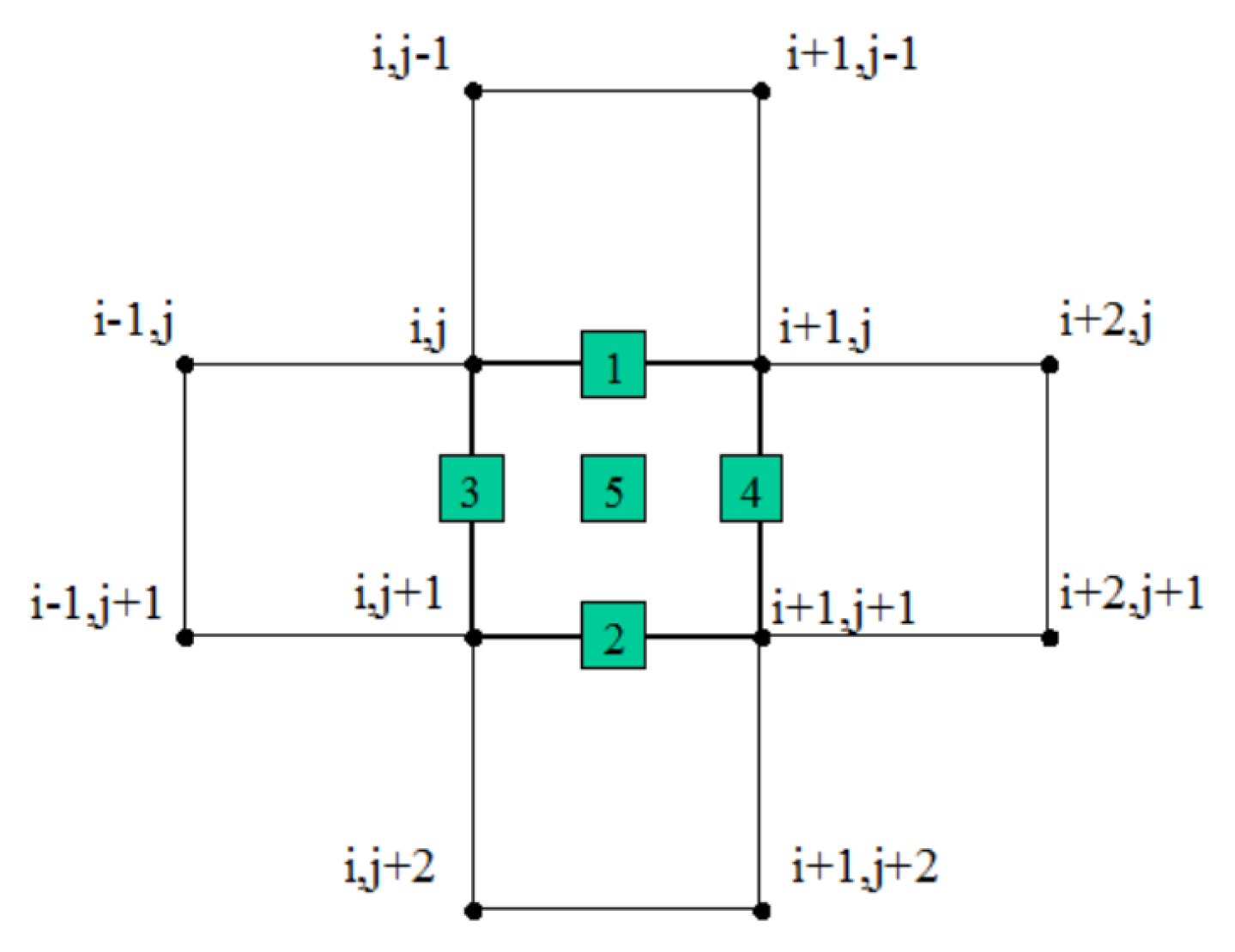
We easily define our prediction operator in $2D$ in the following way. Supposing the data at scale $f^L$ is already known, we compute the data at scale $f^{L+1}$ using the proposed $G_L^{L+1}$ one-dimensional prediction operator defined in Section 3. Since our one-dimensional prediction is local, it is the two-dimensional prediction, as well. In Figure 2, we can see the disposition of the considered cells in order to compute the proposed $2D$ prediction operator $G_L^{L+1}$.

If we suppose that we have the values $f_{i,j}^L,$ then we propose the following calculations to get the needed values $f_{2i+1,2j}^{L+1}$, $f_{2i+1,2j+2}^{L+1}$, $f_{2i,2j+1}^{L+1}$, $f_{2i+2,2j+1}^{L+1}$, $f_{2i+1,2j+1}^{L+1}:$

$$\begin{array}{ccc}\hfill & (1)\hfill & \frac{1}{2}(f_{i,j}^L+f_{i+1,j}^L)-\frac{h^2}{4}G{M}_k(D^{x,j}{f}_i^L,D^{x,j}{f}_{i+1}^L),\hfill \\ \hfill & (2)\hfill & \frac{1}{2}(f_{i,j+1}^L+f_{i+1,j+1}^L)-\frac{h^2}{4}G{M}_k(D^{x,j+1}{f}_i^L,D^{x,j+1}{f}_{i+1}^L),\hfill \\ \hfill & (3)\hfill & \frac{1}{2}(f_{i,j}^L+f_{i,j+1}^L)-\frac{h^2}{4}G{M}_k(D^{i,y}{f}_j^L,D^{i,y}{f}_{j+1}^L),\hfill \\ \hfill & (4)\hfill & \frac{1}{2}(f_{i+1,j}^L+f_{i+1,j+1}^L)-\frac{h^2}{4}G{M}_k(D^{i+1,y}{f}_j^L,D^{i+1,y}{f}_{j+1}^L),\hfill \end{array}$$

(9)

$$\begin{array}{ccc}& (5)& \frac{1}{4}((1)+(2)+(3)+(4)).\end{array}$$

(10)

Of course, the values at the positions $(2i,2j)$ are just projections from the coarser level, i.e., $f_{2i,2j}^{L+1}=f_{i,j}^L.$

Notice that, from the definition, we immediately get that the required properties for the prediction operator are satisfied, just by using Proposition 1. In fact, $\rho =\frac{2+\sqrt[k]{2}}{4}<1$ for $k>1,$$\delta =h^{2}D$, ${||\delta ||}_{\infty }=2$, $C=\frac{\sqrt[k]{2}}{4}.$

With all these ingredients, we can give now the following Theorem regarding the stability of the $2D$ multiresolution transform coming from the use of the $2D$ prediction operator associated to $G_L^{L+1}$ defined through the use of the Generalized means (8) for $k>1.$

Theorem 1.

The $2D$ non-separable multiresolution transform associated with the prediction operator $G_L^{L+1}$ related with the Generalized means $G{M}_k$ for $k>1$ satisfies

$$||f^L-g^L{||}_{\infty }\le \tilde{C}(||f^0-g^0{||}_{\infty }+\sum _{l=1}^L{||e(f)}^l-e{(g)}^l{||}_{\infty }),$$

where $\tilde{C}=1+\frac{{C||\delta ||}_{\infty }}{1-\rho }=\frac{4-\sqrt[k]{2}}{4-2\sqrt[k]{2}}.$ Therefore, we get the stability of the decoding multiresolution transformation.

The proof of this theorem is a particularization of a general proof for prediction operators that contract in one step that can be found in Reference [8].

A Specific Coding Algorithm Controlling the Committed Error

Given a prescribed tolerance $ϵ,$ using Theorem 1, one can control how to carry out the truncation of the details at each scale of the multiresolution pyramid in order to ensure this requirement, that is, having the final committed error bounded by the specified $ϵ$. In this case, one loses control of how much compression is attained in favor of controlling the final error at the decompression stage. We now give a slightly modified version of Algorithm 1 such that the total accumulated error is under control as explained above. Notice that, in order to decompress the signal, one just needs to follow the same decompression Algorithm 2 without any change applied to the truncated version of the multiresolution representation of the data $\tilde{\mu }(f^L).$ We use the following truncation operator $\tilde{e}=tr(e,\delta )$, defined as follows:

$$tr{(e,\delta )}_j:=\left\{\begin{array}{cc}{e}_j& \mathrm{if}|e_j|\ge \delta ,\\ 0& \mathrm{otherwise},\end{array}\right.$$

for all entries ${\tilde{e}}_j$ of the vector $\tilde{e}.$

5. Numerical Experiments

In this section, we offer some numerical tests to compare our proposed $2D$ non-separable multiresolution algorithm with other existing multiresolution transformations in the literature. At the same time, we will verify the numerical stability and the overall performance of the schemes. Let us consider a discrete uniform grid with $65\times 65$ points in the rectangle $[-5,5]\times [-5,5]$ and the function

$$f(x,y):=\left\{\begin{array}{cc}3\frac{cos(\frac{x^2+y^2}{3})}{3+x^2+y^2},\hfill & \mathrm{if}x\le \frac{1}{2}\hfill \\ 3\frac{cos(\frac{x^2+y^2}{3})}{3+x^2+y^2}+10,\hfill & \mathrm{otherwise}.\hfill \end{array}\right.$$

Since $f(x,y)$ is a discontinuous function with a jump along a curve (the straight line $x=\frac{1}{2}$), we can expect that nonlinear methods will work much better in this case than their linear counterparts, which are known to produce artificial maxima and minima around the jump discontinuity. These artificial maxima and minima are not reduced by taking smaller grid sizes when using linear methods. These undesirable features are widely known as Gibbs effects [14].

We consider the discretization of the function by point values $F=(f_{i,j})$ in the given rectangle. From these data, we will perform a multiresolution decomposition, we will keep a percentage of the details, and then we will decode the processed multiresolution version of the data to obtain an approximation to the original data. We take into account the following prediction operators:

• LAG stands for the tensor product multiresolution transform based on fourth order accurate Lagrange prediction operator. This transform is linear and, therefore, stable, but it does not adapt to discontinuities.
• ENO stands for the tensor product multiresolution transform based on fourth order accurate ENO prediction operator. This transform is nonlinear and obtains acceptable resolution of the edges when noise is not present, and the discontinuities are well defined. However, it presents stability problems, forcing to keep the majority of the details to get a appropriate performance.
• $G{M}_1$ stands for the proposed non-separable multiresolution scheme with $k=1.$
• $G{M}_2$ stands for the proposed non-separable multiresolution scheme with $k=2.$
• $G{M}_3$ stands for the proposed non-separable multiresolution scheme with $k=3.$

The last three considered multiresolution transforms $G{M}_1$, $G{M}_2$, $G{M}_3$ are nonlinear by definition and theoretically stable, as proven in Theorem 1.

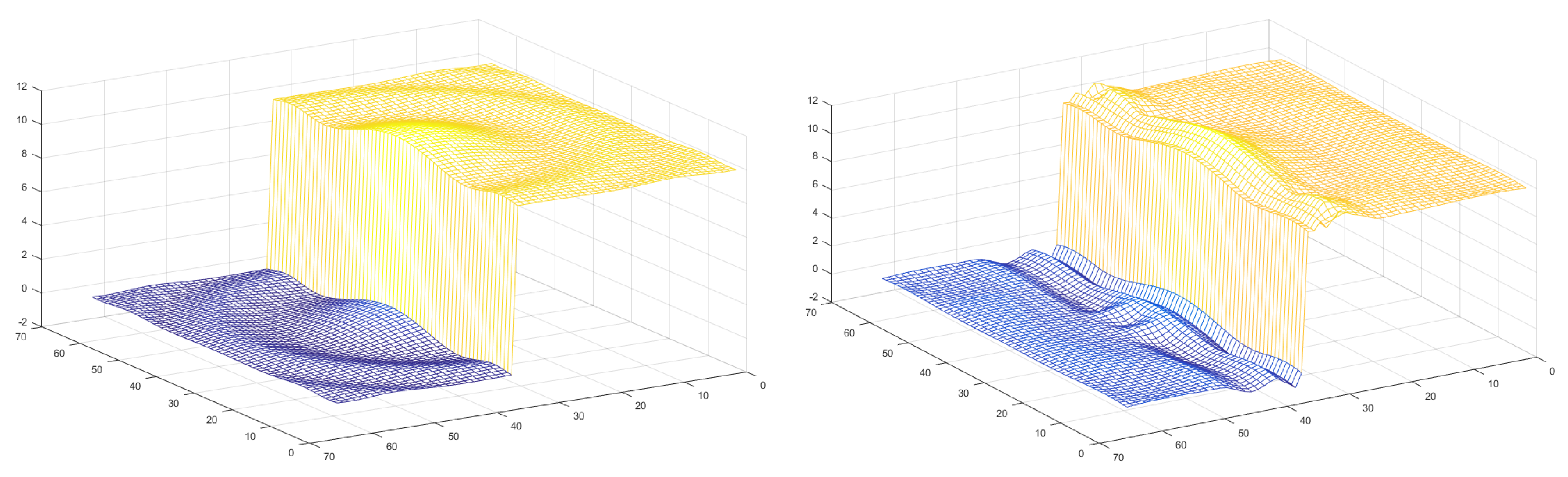
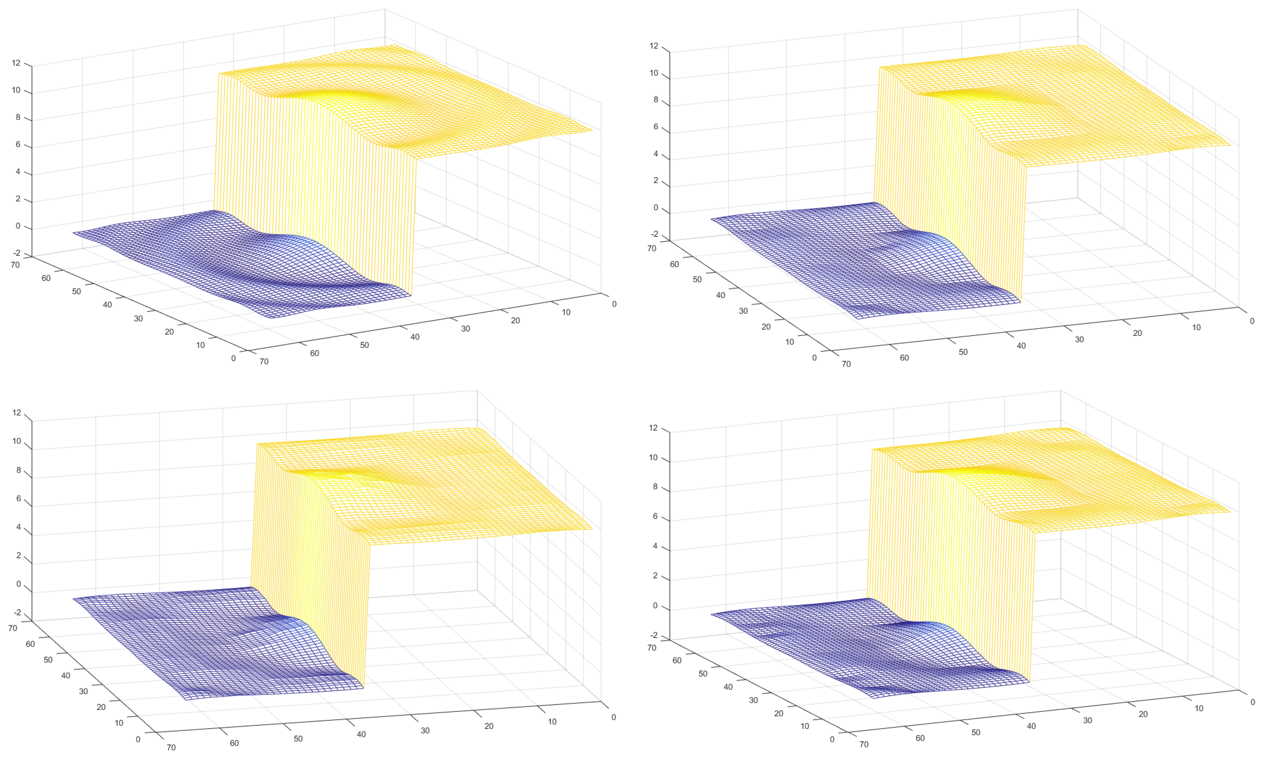
In our experiment, we have descended two scales in the multiresolution algorithm, and we have kept only $7\%$ of the details. In Figure 3, we see the original function to the top-left, and the obtained reconstruction using $LAG$ to the top-right, using $ENO$ to the bottom-left and using $G{M}_1$ to the bottom-right. It is immediate to see how the nonlinear scheme $G{M}_1$ performs better. Gibbs effects are observed in the reconstruction $LAG$. Stability problems are present for $ENO,$ which traduce in undesirable visual effects around the discontinuity. 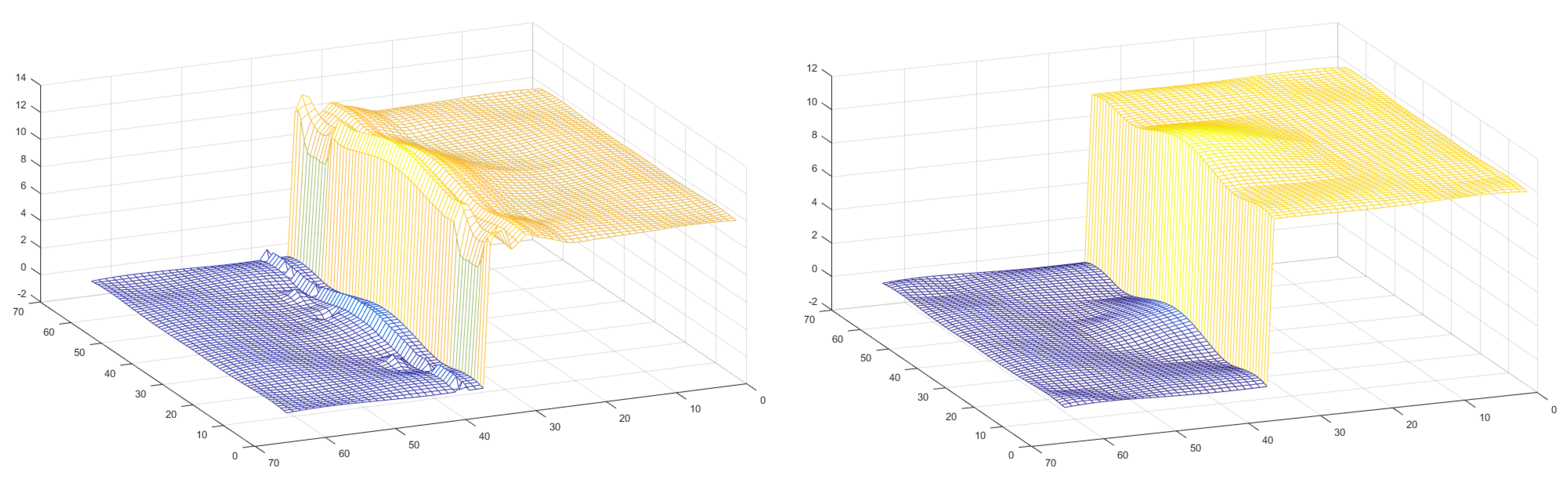In Figure 4, we see how the algorithms $G{M}_2$ and $G{M}_3$ improve progressively the accuracy in the definition of the discontinuity. This fact comes from property of Lemma 2. All these visual appreciations can be reinforced with the numerical results offered in

Table 1. Obtained quality after the compression (93%) and decompression process using 2 scales of different MR algorithms: LAG, ENO, $G{M}_1$, $G{M}_2$, $G{M}_3$ without error control strategies.

%COM	93%
Norm	$||\mathit{F}-\tilde{\mathit{F}}{||}_{\mathbf{1}}$	$||\mathit{F}-\tilde{\mathit{F}}{||}_{\mathbf{2}}$	$||\mathit{F}-\tilde{\mathit{F}}{||}_{\infty }$
LAG	$0.16049$	$0.07714$	$0.98302$
ENO	$0.17761$	$0.13827$	$2.07510$
$G{M}_1$	$0.05075$	$0.00436$	$0.18657$
$G{M}_2$	$0.05379$	$0.00453$	$0.18561$
$G{M}_3$	$0.05140$	$0.00429$	$0.17322$

. In particular, we clearly see the Gibbs effects of $LAG$, the instabilities of $ENO$, and the improvement of $G{M}_k$ with increasing k by paying attention to the fourth column, where the infinity norm of the errors between the original signal and the reconstructed signal are shown. All these computations and graphical representations were carried out using MATLAB under an Intel(R) Core(TM) i7-3770 @ $3.40$ GHz processor with $8.00$ Gb of RAM memory.

Remark 1.

This test could simulate the compression of real geographical data, elevations, or depths of difficult access areas, for instance, in oceanography. The presented methods are designed to work well, especially where cliffs and similar terrain irregularities are encountered.

6. Conclusions and Perspectives

We have defined a new nonlinear reconstruction operator adapted to singularities which is based on the Generalized means $G{M}_k$ for $k\ge 1.$ Using a non-separable strategy, we have defined new nonlinear non-separable $2D$ multiresolution schemes for which the stability is easy to prove (see Reference [8]). In fact, we give a specific stability result for all these presented schemes. The validity of the theoretical results has been tested in a numerical experiment, where one can observe certain improvements for k increasing. This improvement is in agreement with the better obtained theoretical bounds, since the larger k the lower $\sqrt[k]{2}.$ The overall performance of the schemes is quite acceptable, avoiding Gibbs effects and instabilities due to the presence of discontinuities in the original data.