Review of the Lineal Complexity Calculation through Binomial Decomposition-Based Algorithms

Abstract

The ubiquity of smart devices and IoT are the main forces behind the development of cryptographic primitives that preserve the security of this devices, with the resources constraints they face. In this sense, the development of lightweight cryptographic algorithms, where PRNGs are an essential part of them, provides security to all these interconnected devices. In this work, a family of sequence generators with hard characteristics to be analyzed by standard methods is described. Moreover, we introduce an innovative technique for sequence decomposition that allows one to extract useful information on the sequences under study. In addition, diverse algorithms to evaluate the strength of such binary sequences have been introduced and analyzed to show which performs better.

1. Introduction

Sensorization is only one of the latest trends which brings a net of communications around us, as Internet of Things (IoT), and it is said is one of main requirements for third technological revolution. Different critical sectors such as smart-grid, e-health or industrial automation will increase their dependence on this low-cost devices, and with the grow in dependence will also increase the security risks [1,2].

Ubiquitous devices such as IoT are characterized by their constraints on energy consumption, processing power, memory, and size, which makes harder to keep them secure. Combining their network dependability with their low security features, they became the perfect target for gaining control of the applications and systems behind them [3]. a good example where a vulnerable IoT sensor was used to gain control over the whole system can be found here [4].

Different approaches in research [5], 5G [6] or specific calls such as that of NIST for lightweight cryptography primitives [7], are addressing the security of IoT, taking into account the limited resources available on such devices. Lightweight cryptography, with stream ciphers as his core, are the keystones on which the different protocols of communication and orchestration are built [8].

In this work, first we will introduce Linear Feedback Shift Registers (LFSR), key components in stream ciphers, often used as Pseudo Random Number Generators (PRNG). Among the most recent PRNGs based on shift registers, we can list: the Grain-128AEAD [9] a stream cipher supporting authenticated encryption with associated data that includes both Linear and Nonlinear Shift Registers (LFSR and NFSR, respectively), the TinyJAMBU [9] a family of Lightweight Authenticated Encryption Algorithms whose keyed permutation is based on an 128-bit NLFSR or the Espresso [10] a PRNG for 5G wireless communication systems including a 256-bit LFSR and a 20-variable nonlinear output function. the two first generators are second-round candidates in the lightweight crypto standardization process launched by NIST.

Next, we will present the generalized shelf shrinking generator, a particular family of ciphers with strong cryptographic characteristics which remain strong to the standard Berlekamp-Massey Algorithm [11]. Then, we improved an innovative sequence decomposition introduced by Cardell et al. in [12] and will show how it can be used to analyze the properties of binary sequences. Finally, we will compare the different algorithms based on the sequence decomposition, including two novel algorithms based on the symmetry of the binomial sequences and on the B-representation of binary sequences, respectively.

The study of the generalized shelf shrinking generator is not a random choice. Indeed, it produces not only sequences that are hard to analyze by the Berlekamp-Massey algorithm, but also it has been implemented in hardware [13] along on RFID devices [14] and programmable logic devices [15], as a key stream generator. Studying the robustness of these sequences could prevent vulnerabilities on the IoT devices and the services built on them.

This work’s purpose is to effectively compare the binomial decomposition-based algorithms, showing their strengths and possible use-cases. the first contribution of this work is the experimental study of the number of binomial components in a binomial decomposition (parameter r), which allows us to study the complexity of the BD algorithm. In addition, we present the half-interval search algorithm. Despite it being based on our previous design of the folding algorithm [16], In this work we complete the available knowledge on such an algorithm providing a mathematical proof of its behaviour and correctness. the matrix binomial decomposition algorithm is another novelty of this article, which is based on a recent representation of the generalized self-shrunken sequences [17]. Finally, after completing the gaps on the algorithm definitions, the last contribution of our work is the comparison among all the previous algorithms and the discussion about their different use-cases. The paper is organized as follows. Section 2 includes a brief revision of LFSRs and sequence generators based on irregular decimation, a well-known kind of generators including the generalized self-shrinking generator. Section 3 describes the characteristics and generalities of the binomial sequences, binary sequences that constitute the foundations of the last algorithms above mentioned. Section 4 introduces and analyzes four algorithms to calculate the linear complexity of binary sequences: (a) the standard Berlekamp–Massey algorithm, (b) the binomial decomposition BS-algorithm, an improved version of the algorithm developed in [12], which analyzes different properties of the binary sequences, (c) the half-interval search algorithm, a novel proposal based on the symmetry of the binomial sequences and (d) the matrix binomial decomposition or m-BD algorithm based on the product of matrices. Section 5 includes the discussion and extensively comparison among the four previous algorithms, including experiments that test its performance. Finally, conclusions and future research are in Section 6.

2. Shift Registers and the Concept of Linear Complexity

Pseudo-random binary sequences have extensive applications in secure communications, e.g., wireless systems, cryptography, error-correcting codes or circuit testing. Commonly used structures for the generation of such sequences are the Linear Feedback Shift Registers (LFSRs) [18]. In fact, LFSRs are essential components in the design of many sequence generators found in the literature. Good reliability, high speed and easy implementation are some of their practical advantages, which justify a so wide and generalized use. From a theoretical point of view, LFSRs are mathematical models readily analyzable by means of algebraic methods [18].

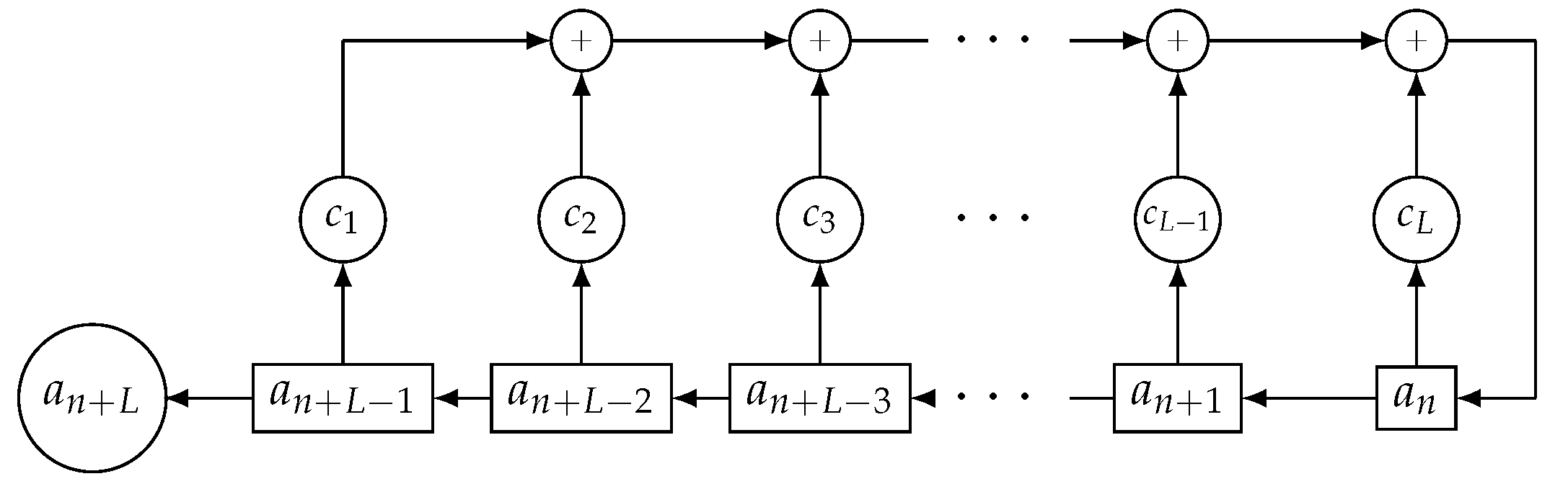
According to Figure 1, an LFSR is made up of the following components:

• L binary stages, which are interconnected and numbered $(0,1,2,\dots ,L-1)$ from left to right. Each stage stores a unique bit.
• The L-degree feedback or connection polynomial

  $$p(x)=x^L+c_1{x}^{L-1}+c_2{x}^{L-2}+\dots +c_{L-1}x+c_L$$

  with coefficients $c_i$ defined in the binary field $c_i\in {\mathbb{F}}_2$.
• A non-zero initial state (stage contents) at the initial instant.

In brief, LFSRs generate sequences by means of successive linear feedbacks and shifts.

The output sequence of an LFSR is a binary sequence $\{a_n\}$$(n=0,1,2,\cdots )$ with $a_n\in {\mathbb{F}}_2$. When the polynomial $p(x)$ is a primitive polynomial [18], then the output sequence is a PN-sequence (or Pseudo-Noise sequence); besides, a PN-sequence has length $l=2^L-1$ bits where $2^{L-1}$ of them are ones and $2^{L-1}-1$ are zeros.

The idea of pseudo-randomness in sequences of finite length implies the difficulty of predicting the subsequent digits of a sequence from the knowledge of the previous ones. a measure of unpredictability is the parameter linear complexity, notated $LC$. Roughly speaking, $LC$ is related with the amount of sequence we need to process in order to recover all the sequence. In terms of security, this amount has to be as large as possible; the recommended value is half the length of the sequence.

The concept of linear complexity of a sequence is closely related to LFSRs. the formal definition of $LC$ is now introduced:

Definition 1.

The linear complexity of a binary sequence $\{s_n\}$$(n=0,1,2,\cdots )$ with $s_n\in {\mathbb{F}}_2$ is the length of the shortest LFSR able to generate such a sequence.

By definition, the $LC$ of a PN-sequence generated by a LFSR with L stages is $LC=L$.

Although LFSRs are in themselves excellent generators of pseudo-random sequence, they are essentially linear structures. This is the reason any kind of non-linearity must be introduced in the process of generation. Non-linear filters, clock-controlled generators, combination generators or dynamic LFSR-based generators are just some of the habitual examples of sequence generators involving non-linearity, see [19,20] and the references cited therein. Particular attention deserves the irregular decimation of PN-sequences as an efficient technique to erase the linearity inherent to LFSRs [21,22]. Among the different examples of decimation-based generators we can enumerate: (1) the shrinking generator [23] with two LFSRs for a mutual decimation, (2) the self-shrinking generator [24] with just one LFSR that decimates itself and (3) the generalized self-shrinking generator [25] that outputs a family of pseudo-random sequences, the so-called generalized self-shrunken sequences (GSS-sequences). Different cryptanalytic attacks against the previous generators can be found in the literature [26,27,28,29,30].

In this work, we focus on binary sequences whose length is a power of 2, characteristic exhibited by many of the sequences from the previous generators.

An LFSR-Based Sequence Generator

A characteristic design of LFSR-based sequence generator is the generalized self-shrinking generator (GSSG). In fact, it is the most representative element in the class of decimation-based generators as well as a practical design with application in low-cost passive RFID tags, see [14].

A GSSG consists of:

(a)

A PN-sequences $\{a_n\}$ generated by an L-stage LFSR and a shifted version of such a sequence, notated $\{b_n\}$. Both sequences are related by the expression $\{b_n\}=\{a_{n+p}\}$, p being an integer. Thus, $\{b_n\}$ is nothing but the PN-sequence $\{a_n\}$ circularly rotated p positions with $(p=0,1,2\dots ,2^L-2)$.

(b)

A simple decimation rule defined as:

$$\left\{\begin{array}{c}\mathrm{If} a_n=1 \mathrm{then} b_n \mathrm{is} \mathrm{output},\hfill \\ \mathrm{If} a_n=0 \mathrm{then} b_n \mathrm{is} \mathrm{discarded} \mathrm{and} \mathrm{no} \mathrm{bit} \mathrm{is} \mathrm{output}.\hfill \end{array}\right.$$

For every p, a new sequence ${\{u_n\}}_p={\{u_0,u_1,u_2,\dots \}}_p$ is generated. Each sequence ${\{u_n\}}_p$ is called the generalized self-shrunken sequence associated with the rotation p. When p ranges in the interval $[0,1,\dots ,2^L-2]$, then we obtain all the elements of the family of GSS-sequences (in total $2^L-1$ elements) based on the PN-sequence $\{a_n\}$.

Some important facts essentially extracted from [25] are enumerated:

• All the generalized self-shrunken sequences are balanced apart from the identically 1 sequence [25] (Theorem 1).
• By construction, the family of generalized self-shrunken sequences consists of $2^L-1$ sequences of $2^{L-1}$ bits each of them. Thus, the length of any generalized sequence will be $2^{L-1}$ or divisors. At any rate, the length of these sequences will always be a power of 2.
• The family of generalized sequences plus the identically null sequence has structure of Abelian group where the group operation is the bit-wise sum mod 2. the neutral element is the identically null sequence and every sequence is its own inverse element [25] (Theorem 2).
• The sequence produced by the self-shrinking generator is a member of this family for $p=2^{L-1}$, see [22].

Moreover, we can add that the $LC$ of every GSS-sequence is upper-bounded by $2^{L-1}-(L-2)$ [31] (Theorem 2). A simple example of GSS-sequences is next introduced.

Example 1.

With a LFSR whose primitive polynomial is $p(x)=x^3+x+1$ and initial state $(1,0,1)$, we can generate the GSS-sequences depicted in

Table 1. Family of generalized sequences for $p(x)=x^3+x+1$.

p-Rotation	$\{{\mathit{b}}_{\mathit{n}}\}$ Sequences	GSS-Sequences
0	$\mathbf{1}$ 0 $\mathbf{1}$ $\mathbf{1}$ $\mathbf{1}$ 0 0	1111
1	$\mathbf{0}$ 1 $\mathbf{1}$ $\mathbf{1}$ $\mathbf{0}$ 0 1	0110
2	$\mathbf{1}$ 1 $\mathbf{1}$ $\mathbf{0}$ $\mathbf{0}$ 1 0	1100
3	$\mathbf{1}$ 1 $\mathbf{0}$ $\mathbf{0}$ $\mathbf{1}$ 0 1	1001
4	$\mathbf{1}$ 0 $\mathbf{0}$ $\mathbf{1}$ $\mathbf{0}$ 1 1	1010
5	$\mathbf{0}$ 0 $\mathbf{1}$ $\mathbf{0}$ $\mathbf{1}$ 1 1	0101
6	$\mathbf{0}$ 1 $\mathbf{0}$ $\mathbf{1}$ $\mathbf{1}$ 1 0	0011
PN-sequence	$\mathbf{1}$ 0 $\mathbf{1}$ $\mathbf{1}$ $\mathbf{1}$ 0 0

. Bits in bold in the sequences $\{b_n\}$ represent the digits of the corresponding GSS-sequence associated with the rotation p. the PN-sequence $\{a_n\}$ with length $l=2^3-1$ and ones in bold appears at the bottom of the table.

3. Binomial Sequences

A new representation of binary sequences in terms of the so-called binomial sequences is now introduced. Such a representation applies only to sequences whose length is a power of 2. Next, we analyze the representation of the GSS-sequences by means of binomial sequences.

3.1. Introduction to Binomial Sequences

The binomial number $\left(\genfrac{}{}{0pt}{}{n}{k}\right)$ ($n,k$ being non-negative integers) is the coefficient of the power $x^k$ in the expansion of the binomial power ${(1+x)}^n$. For $n\ge 0$, it is a well-known fact that $\left(\genfrac{}{}{0pt}{}{n}{0}\right)=1$ while $\left(\genfrac{}{}{0pt}{}{n}{k}\right)=0$ for all $k>n$.

From the binomial coefficients reduced modulo 2, the concept of binomial sequence is defined as follows:

Definition 2.

The k-th binomial sequence $\left\{\left(\genfrac{}{}{0pt}{}{n}{k}\right)\right\}$$(n=0,1,2,\dots )$ is a binary sequence whose elements are binomial coefficients $\left(\genfrac{}{}{0pt}{}{n}{k}\right)$ reduced modulo 2, i.e.,

$${\left\{\left(\genfrac{}{}{0pt}{}{n}{k}\right)\right\}}_{n\ge 0}={\left\{\left(\genfrac{}{}{0pt}{}{0}{k}\right),\left(\genfrac{}{}{0pt}{}{1}{k}\right),\left(\genfrac{}{}{0pt}{}{2}{k}\right),\dots \right\}}_{mod 2},$$

where k is called the index of the binomial sequence.

The k first terms of the binomial sequence are zeros while the term $\left(\genfrac{}{}{0pt}{}{k}{k}\right)$ corresponds to the first 1.

Table 2. Binomial sequences with their lengths $l_k$ and linear complexities $L{C}_k$.

Binom. Coeff.	Binomial Sequences $\{\left(\genfrac{}{}{0pt}{}{\mathit{n}}{\mathit{k}}\right)\}$	Length	Linear Complexity
$\left(\genfrac{}{}{0pt}{}{n}{0}\right)$	$\left\{1,1,1,1,1,1,1,1,\dots \right\}$	$l_0=1$	$L{C}_0=1$
$\left(\genfrac{}{}{0pt}{}{n}{1}\right)$	$\left\{0,1,0,1,0,1,0,1,\dots \right\}$	$l_1=2$	$L{C}_1=2$
$\left(\genfrac{}{}{0pt}{}{n}{2}\right)$	$\left\{0,0,1,1,0,0,1,1,\dots \right\}$	$l_2=4$	$L{C}_2=3$
$\left(\genfrac{}{}{0pt}{}{n}{3}\right)$	$\left\{0,0,0,1,0,0,0,1,\dots \right\}$	$l_3=4$	$L{C}_3=4$
$\left(\genfrac{}{}{0pt}{}{n}{4}\right)$	$\left\{0,0,0,0,1,1,1,1,\dots \right\}$	$l_4=8$	$L{C}_4=5$
$\left(\genfrac{}{}{0pt}{}{n}{5}\right)$	$\left\{0,0,0,0,0,1,0,1,\dots \right\}$	$l_5=8$	$L{C}_5=6$
$\left(\genfrac{}{}{0pt}{}{n}{6}\right)$	$\left\{0,0,0,0,0,0,1,1,\dots \right\}$	$l_6=8$	$L{C}_6=7$
$\left(\genfrac{}{}{0pt}{}{n}{7}\right)$	$\left\{0,0,0,0,0,0,0,1,\dots \right\}$	$l_7=8$	$L{C}_7=8$

shows the binomial sequences $\{\left(\genfrac{}{}{0pt}{}{n}{k}\right)\}$$(k=0,1,\dots ,7)$, with their lengths $l_k$ and linear complexities $L{C}_k$, see [32].

Different properties of the binomial sequences are next enumerated.

• Given the binomial sequence $\left\{\left(\genfrac{}{}{0pt}{}{n}{k}\right)\right\}$ with $k=2^m+i$ where m is a non-negative integer and the index i takes values in the interval $0\le i<2^m$, then we have that [12] (Proposition 3):

  (a)

  The binomial sequence $\{\left(\genfrac{}{}{0pt}{}{n}{k}\right)\}$ has length $l=2^{m+1}$.

  (b)

  The formation rule of this binomial sequence is:

  $${\left\{\left(\genfrac{}{}{0pt}{}{n}{2^m+i}\right)\right\}}_{0\le n<2^{m+1}}=\left\{\begin{array}{cc} 0 \hfill & \mathrm{if} 0\le n<2^m+i,\hfill \\ {\left(\genfrac{}{}{0pt}{}{n}{i}\right)}_{mod 2} \hfill & \mathrm{if} 2^m+i\le n<2^{m+1}.\hfill \end{array}\right.$$

• The linear complexity of the binomial sequence $\left\{\left(\genfrac{}{}{0pt}{}{n}{2^m+i}\right)\right\}$ with m and i defined as above is $LC=2^m+i+1$, see [12] (Theorem 13).
• Every binary sequence ${\{s_n\}}_{n\ge 0}$ whose length is a power of 2 can be written as linear combination of binomial sequences [12] (Theorem 2). This combination is called the Binomial Decomposition of ${\{s_n\}}_{n\ge 0}$. Such a decomposition allows us to analyze fundamental properties of the sequence, e.g., length and linear complexity.
• Given a sequence ${\{s_n\}}_{n\ge 0}$ with binomial decomposition $\{s_n\}={\sum }_{i=1}^r\left\{\left(\genfrac{}{}{0pt}{}{n}{k_i}\right)\right\}$, where $0\le k_1<k_2<\cdots <k_r$ are integer indices, then its linear complexity is given by $LC=k_r+1$, see [12] (Corollary 14).
• Given a sequence ${\{s_n\}}_{n\ge 0}$ with binomial decomposition $\{s_n\}={\sum }_{i=1}^r\left\{\left(\genfrac{}{}{0pt}{}{n}{k_i}\right)\right\}$, where $0\le k_1<k_2<\cdots <k_r$ are integer indices, then its length l is that of the binomial sequence $\left\{\left(\genfrac{}{}{0pt}{}{n}{k_r}\right)\right\}$, i.e., the length of the binomial sequence of maximum index in its binomial decomposition, see [32] (Theorem 1).

All these properties will be used in the algorithms that compute the $LC$ of every binary sequence ${\{s_n\}}_{n\ge 0}$.

In addition, the binomial sequences can be found in the diagonals of the Sierpinski’s triangle reduced modulo 2 [12] (Section 4) as well as in certain linear cellular automata (e.g., linear automata with rules 102 and 60) as it has been studied in [22] (Chapter 3). See the previous references for more details.

3.2. Binomial Decomposition of GSS-Sequences

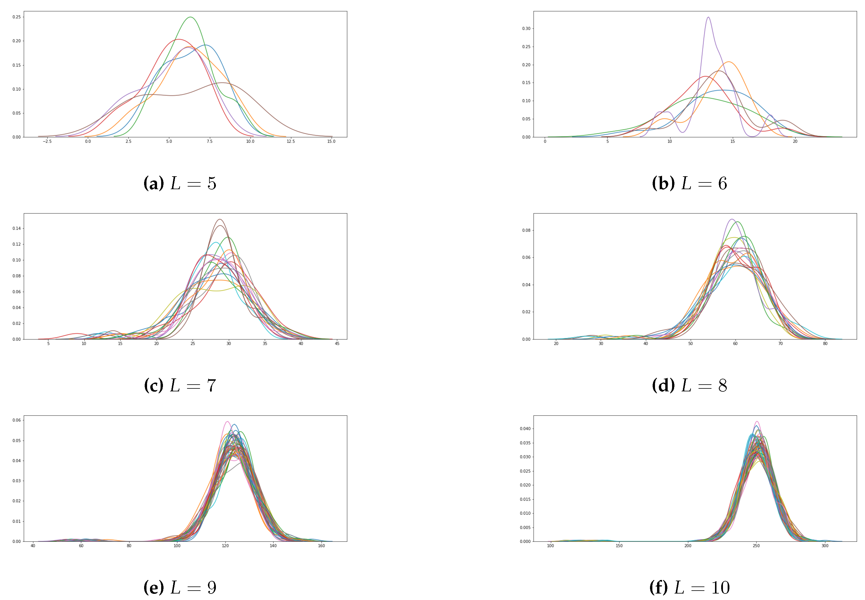
The number of binomial sequences, notated r, In the decomposition of any GSS-sequence has not been previously analyzed in the literature. the parameter is decisive in the comparison among the algorithms of Section 4, since the BD-algorithm complexity depends on the number of binomial sequences. To study the asymptotic behavior of this parameter, some experiments were carried out.

The analyzed sequences in such experiments were all the GSS-sequences coming from LFSRs with primitive feedback polynomials of degree L with L taking values in the interval $[5,10]$. More precisely, we have considered the 6 primitive polynomials of degree 5, the 6 primitive polynomials of degree 6, the 18 primitive polynomials of degree 7, the 16 primitive polynomials of degree 8, the 48 primitive polynomials of degree 9 and the 60 primitive polynomials of degree 10. For each one of these primitive polynomials, the $2^L-1$ GSS-sequences have been generated and decomposed in terms of their binomial sequences. On average, we observed several binomial sequences given by $2^{L-2}$, $\forall L\in [5,10]$.

The plots corresponding to the number of binomial sequences in the decomposition of all these GSS-sequences are depicted in Figure 2. For each chart, the x-axis represents the number of binomial sequences in a specific decomposition (parameter r) while the y-axis counts the number of times r occurs. For a given LFSR, each one of the colors represents all the sequences of the GSS-family generated by such an LFSR. In brief, For each value of L the chart represents the distribution of the parameter r for all the GSS-sequences generated by primitive polynomials of degree L.

The distribution of the number of binomial sequences in the GSS-sequences follows closely a normal distribution. Nevertheless, a smooth tail can be also noticed on the left of the figures, which means that for some GSS-sequences the density of binomial sequences will be lower.

The results of these experiments will be employed in some of the algorithms to compute the $LC$ described in next section.

4. Different Algorithms to Compute the Linear Complexity of a Sequence

In this section, we introduce different algorithms (both novel and already known algorithms) to compute the $LC$ of any binary sequence with length $l=2^m$, m being a non-negative integer. Analysis, foundations and characteristics of each algorithm are described in the subsequent sections.

Throughout the next sections, the following notation will be systematically used.

• For the sake of readability, In the sequel the binomial coefficient $\left(\genfrac{}{}{0pt}{}{n}{k}\right)$ just denotes the k-$th$ binomial sequence.
• The term ${\left(\genfrac{}{}{0pt}{}{n}{k}\right)}_{i,j}$ represents the sub-sequence of $\left(\genfrac{}{}{0pt}{}{n}{k}\right)$ between the i-$th$ and j-$th$ bits.
• The term ${\left(\genfrac{}{}{0pt}{}{n}{k}\right)}_j$ stands for the sub-sequence corresponding to the j first bits of $\left(\genfrac{}{}{0pt}{}{n}{k}\right)$.

4.1. Berlekamp-Massey Algorithm

The most general and well-known method of computing the linear complexity of binary sequences is the Berlekamp-Massey algorithm [11]. Such an algorithm can be applied to sequences of any length, not only to sequences whose length is a power of 2. For a fixed binary sequence, this algorithm processes bit-by-bit the successive digits until it finds the shortest LFSR able to generate the whole sequence. At each particular step, the Berlekamp-Massey algorithm computes the length and the feedback polynomial of the shortest LFSR that produces the sub-sequence analyzed up to that particular bit. Both LFSR length and feedback polynomial degree will always be greater than those of the previous step.

To get the final value of $LC$, this algorithm has to process several bits equal to twice the value of the linear complexity of the sequence under consideration. For sequences whose $LC$ is close to their length l, e.g., the GSS-sequences [22], the Berlekamp-Massey algorithm will process approximately $2\ast l$ bits of each sequence with a computational complexity of $O(l^2)$, see [33].

4.2. Binomial Decomposition Algorithm or BD-Algorithm

To compute the $LC$ of a given sequence, the BD-algorithm [12] provides one with a simple procedure to determine the binomial decomposition of such a sequence. the mathematical results enumerated in the Section 3.1 constitute the core of this algorithm. More precisely, two properties are taken into account:

• According to Item 3 (in Section 3.1), the sequence $seq$ of length $l=2^m$ can be decomposed into r binomial sequences of the form:

  $$seq=\left(\genfrac{}{}{0pt}{}{n}{k_1}\right)+\cdots +\left(\genfrac{}{}{0pt}{}{n}{k_r}\right).$$
• According to Item 4 (in Section 3.1), the lineal complexity of $seq$ is that of the binomial sequence of maximum index $\left(\genfrac{}{}{0pt}{}{n}{k_r}\right)$ in its binomial decomposition. Since the indices of the binomial sequences are written in increasing order, then $LC$ is computed by means of the following equation:

  $$LC=k_r+1.$$

  (1)

The result of the previous properties is the algorithm described in Algorithm 1. Indeed, it takes as input the sequence $seq$ and checks for the bits that equal 1. If $se{q}_i$ = 1, then it bit-wise sums the sequence $seq$ with the binomial sequence $\left(\genfrac{}{}{0pt}{}{n}{i}\right)$, so that $seq=seq+\left(\genfrac{}{}{0pt}{}{n}{i}\right)$. the procedure stops when all the binomial sequences in the decomposition have been determined or, equivalently, when the resulting sequence $seq$ is the identically null sequence. the algorithm outputs the binomial decomposition of the sequence under consideration as well as the value of its $LC$, via the Equation (1).

Algorithm 1 The BD-algorithm.

Require:$seq$: the sequence to be analyzed

$binom=[\varnothing ]$, $k_r=0$

for $i=0; i<length(seq); i$++ do

if $se{q}_i==1$ then

$seq+=\left(\genfrac{}{}{0pt}{}{n}{i}\right)$

$binom.add(i)$

$k_r=i$

end if

end for

return $binom$ and $LC=k_r+1$: binomial decomposition and $LC$ of $seq$.

A step-by-step application of Algorithm 1 to the binomial decomposition of $se{q}_{16}=\{0001110110001011\}$ with $l=2^4$ is depicted in

Table 3. A step-by-step application of the BD-algorithm to $se{q}_{16}$.

Step	Op.	Seq.	Bit Position
			0	4	8	12
1		$seq$	0 0 0 1	1 1 0 1	1 0 0 0	1 0 1 1
	+	$\left(\genfrac{}{}{0pt}{}{n}{3}\right)$	0 0 0 1	0 0 0 1	0 0 0 1	0 0 0 1
2	=	$seq$	0 0 0 0	1 1 0 0	1 0 0 1	1 0 1 0
	+	$\left(\genfrac{}{}{0pt}{}{n}{4}\right)$	0 0 0 0	1 1 1 1	0 0 0 0	1 1 1 1
3	=	$seq$	0 0 0 0	0 0 1 1	1 0 0 1	0 1 0 1
	+	$\left(\genfrac{}{}{0pt}{}{n}{6}\right)$	0 0 0 0	0 0 1 1	0 0 0 0	0 0 1 1
4	=	$seq$	0 0 0 0	0 0 0 0	1 0 0 1	0 1 1 0
	+	$\left(\genfrac{}{}{0pt}{}{n}{8}\right)$	0 0 0 0	0 0 0 0	1 1 1 1	1 1 1 1
5	=	$seq$	0 0 0 0	0 0 0 0	0 1 1 0	1 0 0 1
	+	$\left(\genfrac{}{}{0pt}{}{n}{9}\right)$	0 0 0 0	0 0 0 0	0 1 0 1	0 1 0 1
6	=	$seq$	0 0 0 0	0 0 0 0	0 0 1 1	1 1 0 0
	+	$\left(\genfrac{}{}{0pt}{}{n}{10}\right)$	0 0 0 0	0 0 0 0	0 0 1 1	0 0 1 1
7	=	$seq$	0 0 0 0	0 0 0 0	0 0 0 0	1 1 1 1
	+	$\left(\genfrac{}{}{0pt}{}{n}{12}\right)$	0 0 0 0	0 0 0 0	0 0 0 0	1 1 1 1
end	=	$seq$	0 0 0 0	0 0 0 0	0 0 0 0	0 0 0 0
$seq=\left(\genfrac{}{}{0pt}{}{n}{3}\right)+\left(\genfrac{}{}{0pt}{}{n}{4}\right)+\left(\genfrac{}{}{0pt}{}{n}{6}\right)+\left(\genfrac{}{}{0pt}{}{n}{8}\right)+\left(\genfrac{}{}{0pt}{}{n}{9}\right)+\left(\genfrac{}{}{0pt}{}{n}{10}\right)+\left(\genfrac{}{}{0pt}{}{n}{12}\right)$
$LC=k_r+1=12+1=13$

.

Recall that the BD-algorithm computes $LC$ after processing 13 bits of $se{q}_{16}$ while the Berlekamp-Massey algorithm needs $2\ast 13=26$ bits. In fact, the BD-algorithm performs the bit-wise sum of two sequences of l bits, i.e., l operations, For each binomial sequence that appears in the binomial decomposition. Thus, its computational complexity is $O(r\ast l)$, where r is the number of binomial sequences in the decomposition of the analyzed sequence with $r\ll l$.

Next, we show how the BD-algorithm can be improved and its complexity reduced.

Improvement of the BD-Algorithm

If we avoid the sum of the sub-sequences identically null, then the performance of this algorithm clearly improved. Due to the properties of the binomial coefficients described in Section 3.1, we know that $\left(\genfrac{}{}{0pt}{}{n}{k}\right)=0$ for all $n<k$. At the same time, notice that at the i-$th$ step of the algorithm the $k_i$ first terms of $seq$ are zeros.

Therefore, combining these two facts the number of operations is substantially reduced. When the first 1 in the i-$th$ position of $seq$ is detected, then the algorithm bit-wise sums both sequences exclusively between the i-$th$ and $(l-1)$-$th$ bits, i.e., ($se{q}_{i,l-1}+{\left(\genfrac{}{}{0pt}{}{n}{i}\right)}_{i,l-1}$), as the headers of both sequences (until the $(i-1)$-$th$ bit) are zeros.

In this way, the number of additions at each step is incrementally reduced:

$$\sum _{i=1}^r(l-k_i)<r\ast l.$$

Moreover, For sequences whose $LC$ is upper bounded the algorithm performance can be even improved. In fact, In that case we do not need to check any other bit after the index corresponding to this upper bound. For example, every sequence produced by a generalized self-shrinking generator with LFSR of length L has a $LC$ upper bounded by $L{C}_{max}=2^{L-1}-(L-2)$, [31]. In that case, the maximum index $k_{max}$ in its binomial decomposition is $k_{max}=l-logl$, $l=2^{L-1}$ being the sequence length. Hence, the final number of operations is again reduced to:

$$\sum _{i=1}^r(k_{max}-k_i)<\sum _{i=1}^r(l-k_i)<r\ast l.$$

The code of Algorithm 1 is just upgraded by converting the bit-wise sum of both sequences into the expression $seq=se{q}_{i,k_{max}}+{\left(\genfrac{}{}{0pt}{}{n}{i}\right)}_{i,k_{max}}$, with $k_{max}$ defined as before.

In brief, For this family of sequences the BD-algorithm requires $l-logl$ bits of each sequence to compute its $LC$ with a computational complexity less than $O(r\ast l)$.

4.3. Half-Interval Search Algorithm

In this subsection a novel algorithm to compute the $LC$, the so-called half-interval search algorithm, is described. Such an algorithm takes full advantage of the binomial sequence symmetry. a preliminary version of this algorithm by the same authors was introduced in [16,34]. First of all, we study the symmetry properties of the Binomial sequences.

4.3.1. Symmetry of the Binomial Sequences

In fact, the symmetry of these sequences gives rise to the following results.

Theorem 1.

Let ${\left(\genfrac{}{}{0pt}{}{n}{k}\right)}_l$ denote the l first bits of the binomial sequence $\left(\genfrac{}{}{0pt}{}{n}{k}\right)$ with $l=2^m$, m being a positive integer. Such a sub-sequence can be divided into two new sub-sequences of length $\frac{l}{2}$:

$${\left(\genfrac{}{}{0pt}{}{n}{k}\right)}_l=\left({\left(\genfrac{}{}{0pt}{}{n}{k}\right)}_{0,\frac{l}{2}-1},{\left(\genfrac{}{}{0pt}{}{n}{k}\right)}_{\frac{l}{2},l-1}\right),$$

(2)

then, two different configurations may appear:

• If k the index of the binomial sequence is $k<\frac{l}{2}$, then the two sub-sequences in Equation (2) are equal.
• If k the index of the binomial sequence is $k\ge \frac{l}{2}$, then the two sub-sequences in Equation (2) are written as:

  $${\left(\genfrac{}{}{0pt}{}{n}{k}\right)}_l=\left(zero{s}_{\frac{l}{2}},{\left(\genfrac{}{}{0pt}{}{n}{i}\right)}_{\frac{l}{2}}\right),$$

  (3)

  where $zero{s}_{\frac{l}{2}}$ represents the sub-sequence identically null of length $\frac{l}{2}$ and i is an integer satisfying $0\le i<2^{m-1}$.

Proof. 

Both cases are proved separately.

• Since $k<\frac{l}{2}$, then k can be written as $k=2^j+i$, where j and i are non-negative integers such that $j<m-1$ and $0\le i<2^j$. According to Item 1(a) in Section 3.1, the binomial sequence $\left(\genfrac{}{}{0pt}{}{n}{k}\right)=\left(\genfrac{}{}{0pt}{}{n}{2^j+i}\right)$ has length $\tilde{l}=2^{j+1}$ where the maximum length is ${\tilde{l}}_{max}=2^{m-1}$ when $j=m-2$ and the minimum length ${\tilde{l}}_{min}=2^0$ when $j=0$. At any rate, $\tilde{l}$ is a power of 2 as well as $\tilde{l}<2^m$ and, therefore, the first and second sub-sequences in Equation (2) are equal.
• Since $k\ge \frac{l}{2}=2^{m-1}$, then k can be written as $k=2^{m-1}+i$ with $0\le i<2^{m-1}$. According to Item 1(a) in Section 3.1, the binomial sequence $\left(\genfrac{}{}{0pt}{}{n}{k}\right)=\left(\genfrac{}{}{0pt}{}{n}{2^{m-1}+i}\right)$ has length $\tilde{l}=l=2^m$. Moreover, according to Item 1(b) in Section 3.1

  $${\left(\genfrac{}{}{0pt}{}{n}{k}\right)}_{\frac{l}{2},l-1}={\left(\genfrac{}{}{0pt}{}{n}{2^{m-1}+i}\right)}_{\frac{l}{2},l-1}={\left(\genfrac{}{}{0pt}{}{n}{i}\right)}_{\frac{l}{2}}.$$
  Thus, the sub-sequence ${\left(\genfrac{}{}{0pt}{}{n}{k}\right)}_l$ satisfies the Equation (3) as well as the $\frac{l}{2}$ first terms are zeros.

   □

In

Table 4. Theorem 1 applied to the binomial decomposition of $se{q}_{16}$.

seq	0 0 0 1	1 1 0 1	1 0 0 0	1 0 1 1
${\left(\genfrac{}{}{0pt}{}{n}{3}\right)}_l=({\left(\genfrac{}{}{0pt}{}{n}{3}\right)}_{\frac{l}{2}},{\left(\genfrac{}{}{0pt}{}{n}{3}\right)}_{\frac{l}{2}})$	0 0 0 1	0 0 0 1	0 0 0 1	0 0 0 1
${\left(\genfrac{}{}{0pt}{}{n}{4}\right)}_l=({\left(\genfrac{}{}{0pt}{}{n}{4}\right)}_{\frac{l}{2}},{\left(\genfrac{}{}{0pt}{}{n}{4}\right)}_{\frac{l}{2}})$	0 0 0 0	1 1 1 1	0 0 0 0	1 1 1 1
${\left(\genfrac{}{}{0pt}{}{n}{6}\right)}_l=({\left(\genfrac{}{}{0pt}{}{n}{6}\right)}_{\frac{l}{2}},{\left(\genfrac{}{}{0pt}{}{n}{6}\right)}_{\frac{l}{2}})$	0 0 0 0	0 0 1 1	0 0 0 0	0 0 1 1
${\left(\genfrac{}{}{0pt}{}{n}{8}\right)}_l=(zero{s}_{\frac{l}{2}},{\left(\genfrac{}{}{0pt}{}{n}{0}\right)}_{\frac{l}{2}})$	0 0 0 0	0 0 0 0	1 1 1 1	1 1 1 1
${\left(\genfrac{}{}{0pt}{}{n}{9}\right)}_l=(zero{s}_{\frac{l}{2}},{\left(\genfrac{}{}{0pt}{}{n}{1}\right)}_{\frac{l}{2}})$	0 0 0 0	0 0 0 0	0 1 0 1	0 1 0 1
${\left(\genfrac{}{}{0pt}{}{n}{10}\right)}_l=(zero{s}_{\frac{l}{2}},{\left(\genfrac{}{}{0pt}{}{n}{2}\right)}_{\frac{l}{2}})$	0 0 0 0	0 0 0 0	0 0 1 1	0 0 1 1
${\left(\genfrac{}{}{0pt}{}{n}{12}\right)}_l=(zero{s}_{\frac{l}{2}},{\left(\genfrac{}{}{0pt}{}{n}{4}\right)}_{\frac{l}{2}})$	0 0 0 0	0 0 0 0	0 0 0 0	1 1 1 1
$se{q}_{16}=\left(\genfrac{}{}{0pt}{}{n}{3}\right)+\left(\genfrac{}{}{0pt}{}{n}{4}\right)+\left(\genfrac{}{}{0pt}{}{n}{6}\right)+\left(\genfrac{}{}{0pt}{}{n}{8}\right)+\left(\genfrac{}{}{0pt}{}{n}{9}\right)+\left(\genfrac{}{}{0pt}{}{n}{10}\right)+\left(\genfrac{}{}{0pt}{}{n}{12}\right)$

, where $\frac{l}{2}=8$, the binomial sequences $\left(\genfrac{}{}{0pt}{}{n}{3}\right),\left(\genfrac{}{}{0pt}{}{n}{4}\right)$ and $\left(\genfrac{}{}{0pt}{}{n}{6}\right)$ correspond to the condition (1) in Theorem 1, where the eight first bits are repeated, while the binomial sequences $\left(\genfrac{}{}{0pt}{}{n}{8}\right),\left(\genfrac{}{}{0pt}{}{n}{9}\right),\left(\genfrac{}{}{0pt}{}{n}{10}\right)$ and $\left(\genfrac{}{}{0pt}{}{n}{12}\right)$ correspond to the condition (2) in the same theorem with $k\ge 8$.

Next result introduces an interesting characteristic of the sub-sequence ${\left(\genfrac{}{}{0pt}{}{n}{k}\right)}_{\frac{l}{2},l-1}$, which can be converted into another binomial sequence.

Proposition 1.

The sub-sequence ${\left(\genfrac{}{}{0pt}{}{n}{k}\right)}_{\frac{l}{2},l-1}$ that is the second sub-sequence of ${\left(\genfrac{}{}{0pt}{}{n}{k}\right)}_l$ in Equation (2) with $k\ge \frac{l}{2}$ can be written as:

$${\left(\genfrac{}{}{0pt}{}{n}{k}\right)}_{\frac{l}{2},l-1}={\left(\genfrac{}{}{0pt}{}{n}{k-\frac{l}{2}}\right)}_{\frac{l}{2}}.$$

Proof. 

According to the previous properties of the binomial sequences, we write:

$${\left(\genfrac{}{}{0pt}{}{n}{k}\right)}_{\frac{l}{2},l-1}={\left(\genfrac{}{}{0pt}{}{n}{2^{m-1}+i}\right)}_{\frac{l}{2},l-1}={\left(\genfrac{}{}{0pt}{}{n}{i}\right)}_{\frac{l}{2}}={\left(\genfrac{}{}{0pt}{}{n}{k-2^{m-1}}\right)}_{\frac{l}{2}}={\left(\genfrac{}{}{0pt}{}{n}{k-\frac{l}{2}}\right)}_{\frac{l}{2}}.$$

□

This will be the notation used in the sequel.

The sub-sequences ${\left(\genfrac{}{}{0pt}{}{n}{k}\right)}_l$ can be classified into two disjoint sets depending on the value of the index k, as explained in Algorithm 2. In the first case, only the first half of the sub-sequence must be computed $(0\le n<\frac{l}{2})$ as the second half is exactly the same. In the second case, it is precisely the second half of the sub-sequence which has to be computed $(\frac{l}{2}\le n<l)$, since the $\frac{l}{2}$ first bits are zeros.

Algorithm 2 Classification of the Binomial sequences.

Given the sub-sequence ${\left(\genfrac{}{}{0pt}{}{n}{k}\right)}_l$:

if $k<\frac{l}{2}$ then

${\left(\genfrac{}{}{0pt}{}{n}{k}\right)}_l:=({\left(\genfrac{}{}{0pt}{}{n}{k}\right)}_{\frac{l}{2}},{\left(\genfrac{}{}{0pt}{}{n}{k}\right)}_{\frac{l}{2}})$

else

${\left(\genfrac{}{}{0pt}{}{n}{k}\right)}_l:=(zero{s}_{\frac{l}{2}},{\left(\genfrac{}{}{0pt}{}{n}{k-\frac{l}{2}}\right)}_{\frac{l}{2}})$

end if

According to the previous classification, a matrix representation of the binomial decomposition is now introduced:

$$\left(\begin{array}{c}\left(\genfrac{}{}{0pt}{}{n}{k_1}\right)\\ ⋮\\ \left(\genfrac{}{}{0pt}{}{n}{k_r}\right)\end{array}\right)={\left(\begin{array}{c}\begin{array}{c}\left(\genfrac{}{}{0pt}{}{n}{k_1}\right)\\ ⋮\\ \left(\genfrac{}{}{0pt}{}{n}{k_{i-1}}\right)\\ \left(\genfrac{}{}{0pt}{}{n}{k_i}\right)\\ ⋮\\ \left(\genfrac{}{}{0pt}{}{n}{k_r}\right)\end{array}\end{array}\right)}_{k_{i-1}<\frac{l}{2}\le k_i}=\left(\begin{array}{c}\begin{array}{cc}{\left(\genfrac{}{}{0pt}{}{n}{k_1}\right)}_{\frac{l}{2}}& {\left(\genfrac{}{}{0pt}{}{n}{k_1}\right)}_{\frac{l}{2}}\\ ⋮& ⋮\\ {\left(\genfrac{}{}{0pt}{}{n}{k_{i-1}}\right)}_{\frac{l}{2}}& {\left(\genfrac{}{}{0pt}{}{n}{k_{i-1}}\right)}_{\frac{l}{2}}\\ zero{s}_{\frac{l}{2}}& {\left(\genfrac{}{}{0pt}{}{n}{k_i-\frac{l}{2}}\right)}_{\frac{l}{2}}\\ ⋮& ⋮\\ zero{s}_{\frac{l}{2}}& {\left(\genfrac{}{}{0pt}{}{n}{k_r-\frac{l}{2}}\right)}_{\frac{l}{2}}\end{array}\end{array}\right)=\left(\begin{array}{c}\begin{array}{cc}{M}_0& M_1\\ M_2& M_3\end{array}\end{array}\right).$$

(4)

The different sub-matrices of the matrix representation in (4) are described as follows:

• $M_0$ and $M_1$ are $((i-1)\times \frac{l}{2})$ sub-matrices that, according to Theorem 1, satisfy the equality $M_0=M_1$.
• $M_2$ is the $((r-i+1)\times \frac{l}{2})$ identically null sub-matrix.
• $M_3$ is the $((r-i+1)\times \frac{l}{2})$ sub-matrix representing the decomposition of a new sequence of length $\frac{l}{2}$ coming from the bit-wise sum of the two halves of $seq$. Therefore, from $M_3$ the matrix representation can be extended recursively.

$$\left(\begin{array}{c}\begin{array}{cc}{M}_0& M_1\\ M_2& M_3\end{array}\end{array}\right)=\left(\begin{array}{c}\begin{array}{cc}{M}_0& M_1\\ M_2& \begin{array}{cc}{M}_{3,0}& M_{3,1}\\ M_{3,2}& M_{3,3}\end{array}\end{array}\end{array}\right)=\left(\begin{array}{c}\begin{array}{cc}{M}_0& M_1\\ M_2& \begin{array}{cc}{M}_{3,0}& M_{3,1}\\ M_{3,2}& \begin{array}{cc}{M}_{3,3,0}& M_{3,3,1}\\ M_{3,3,2}& M_{3,3,3}\end{array}\end{array}\end{array}\end{array}\right)=\dots$$

(5)

In fact, take $M_3$ and repeat the same process until the length of the resulting sequence equals 1 and, consequently, the sequence cannot be divided anymore.

Thus, the half-interval search algorithm takes fully advantage of the symmetry properties of the binomial sequences and reduces recursively the length of the sequence to be analyzed, see Equation (5).

A numerical example of the matrix representation is next introduced.

Example 2.

For the sequence $se{q}_{16}=\{0001110110001011\}$, the matrix representation of its binomial decomposition is:

$$\left(\begin{array}{c}\left(\genfrac{}{}{0pt}{}{n}{3}\right)\\ \left(\genfrac{}{}{0pt}{}{n}{4}\right)\\ \left(\genfrac{}{}{0pt}{}{n}{6}\right)\\ \left(\genfrac{}{}{0pt}{}{n}{8}\right)\\ \left(\genfrac{}{}{0pt}{}{n}{9}\right)\\ \left(\genfrac{}{}{0pt}{}{n}{10}\right)\\ \left(\genfrac{}{}{0pt}{}{n}{12}\right)\end{array}\right)=\left(\begin{array}{c}\begin{array}{cccc}0001& 0001& 0001& 0001\\ 0000& 1111& 0000& 1111\\ 0000& 0011& 0000& 0011\\ 0000& 0000& 1111& 1111\\ 0000& 0000& 0101& 0101\\ 0000& 0000& 0011& 0011\\ 0000& 0000& 0000& 1111\end{array}\end{array}\right)=\left(\begin{array}{c}\begin{array}{cc}{M}_0& M_1\\ M_2& M_3\end{array}\end{array}\right),$$

where

$$M_3=\left(\begin{array}{cc}{M}_{3,0}& M_{3,1}\\ M_{3,2}& M_{3,3}\end{array}\right)=\left(\begin{array}{c}\begin{array}{cc}1111& 1111\\ 0101& 0101\\ 0011& 0011\\ 0000& 1111\end{array}\end{array}\right),$$

and

$$M_{3,3}=\left(\begin{array}{cc}{M}_{3,3,0}& M_{3,3,1}\\ M_{3,3,2}& M_{3,3,3}\end{array}\right)=\left(\begin{array}{c}\begin{array}{cc}11& 11\\ \varnothing & \varnothing \end{array}\end{array}\right).$$

When the two halves of $seq$ are bit-wise summed, then the binomial sequences $\left(\genfrac{}{}{0pt}{}{n}{3}\right)$, $\left(\genfrac{}{}{0pt}{}{n}{4}\right)$ and $\left(\genfrac{}{}{0pt}{}{n}{6}\right)$ with repeated sub-sequences are cancelled. Thus, we have a new $seq$ of length $\frac{l}{2}=8$ including the binomial sequences $\left(\genfrac{}{}{0pt}{}{n}{8}\right)$, $\left(\genfrac{}{}{0pt}{}{n}{9}\right)$, $\left(\genfrac{}{}{0pt}{}{n}{10}\right)$ and $\left(\genfrac{}{}{0pt}{}{n}{12}\right)$. When the two halves of the resulting $seq$ are bit-wise summed again, then we have a new $seq$ of length $\frac{l}{4}=4$ and the binomial sequences $\left(\genfrac{}{}{0pt}{}{n}{8}\right)$, $\left(\genfrac{}{}{0pt}{}{n}{9}\right)$ and $\left(\genfrac{}{}{0pt}{}{n}{10}\right)$ with repeated sub-sequences are cancelled. The only resulting binomial sequence is $\left(\genfrac{}{}{0pt}{}{n}{12}\right)$ what means that $LC=12+1$.

4.3.2. Description of the Half-Interval Search Algorithm

From the symmetry properties of the binomial sequences, the half-interval search algorithm locates the binomial sequence of maximum index to compute the $LC$. At each step, it bit-wise sums both halves of the sequence. If the result is different from zero, then it performs the same procedure with the resulting sequence. Otherwise, it takes half the sequence obtained in the previous step to apply the same procedure. When only one bit is left the Algorithm stops.

The pseudo-code of the algorithm, for a given binary sequence of length $l=2^m$ can be found in Algorithm 3.

Algorithm 3 The half-interval search Algorithm

Require:$seq$: sequence to be analyzed

$k=0$

while $length(seq)>1$ do

$l=length(seq)$

sum = $se{q}_{0,\frac{l}{2}-1}$ + $se{q}_{\frac{l}{2},l-1}$

if $sum\ne 0_{\frac{l}{2}}$ then

$seq=sum$

$k+=\frac{l}{2}$

else

$seq=se{q}_{0,\frac{l}{2}-1}$

end if

end while

return k: maximum index k and $LC$ of $seq$.

At every step, the algorithm reduces by 2 the length of $seq$. The total number of steps is $logl$ and the total number of operations for a sequence $seq$ with length $l=2^m$ is:

$$\frac{l}{2}+\frac{l}{4}+\frac{l}{8}+\frac{l}{16}+\cdots =\sum _{i=1}^{logl}\frac{l}{2^i}\approx l$$

Next, an example of how the half-interval algorithm works is introduced.

Example 3.

Taking the sequence of the previous sub-sections we have:

Input: $se{q}_{16}$ = 00011101 10001011

• Step 1: $\begin{array}{cc}\begin{array}{}\\ \\ sum=\end{array}& \begin{array}{ccc}& 0001& 1101\\ +& 1000& 1011\\ & 1001& 0110\end{array}\end{array}$

As $sum$ = $1001 0110\ne zero{s}_8$, then $seq$ = $sum$ = $1001 0110$ and k = 8.

At this step, the binomial sequences $\left(\genfrac{}{}{0pt}{}{n}{3}\right)$, $\left(\genfrac{}{}{0pt}{}{n}{4}\right)$ and $\left(\genfrac{}{}{0pt}{}{n}{6}\right)$ are cancelled.

• Step 2: $\begin{array}{cc}\begin{array}{}\\ \\ sum=\end{array}& \begin{array}{ccc}& 10& 01\\ +& 01& 10\\ & 11& 11\end{array}\end{array}$

As $sum$ = $11 11\ne zero{s}_4$, then $seq$ = $sum$ = $11 11$ and k = $8+4=12$.

At this step, the binomial sequences $\left(\genfrac{}{}{0pt}{}{n}{8}\right)$, $\left(\genfrac{}{}{0pt}{}{n}{9}\right)$ and $\left(\genfrac{}{}{0pt}{}{n}{10}\right)$ are cancelled.

• Step 3: $\begin{array}{cc}\begin{array}{}\\ \\ sum=\end{array}& \begin{array}{ccc}& 1& 1\\ +& 1& 1\\ & 0& 0\end{array}\end{array}$

As $sum=zero{s}_2$, then $seq$ = $1 1$.

At this step, there is no binomial sequence cancellation and the remaining binomial sequence is $\left(\genfrac{}{}{0pt}{}{n}{12}\right)$.

• Step 4: $\begin{array}{cc}\begin{array}{}\\ \\ sum=\end{array}& \begin{array}{cc}& 1\\ +& 1\\ & 0\end{array}\end{array}$

As $sum=0$, then $seq$ = 1.

At this step, $length(seq)=1$ and the algorithm stops.

• Output: the maximum binomial sequence $\left(\genfrac{}{}{0pt}{}{n}{12}\right)\Rightarrow LC=k+1=12+1=13$.

4.4. Matrix Binomial Decomposition or m-BD Algorithm

This algorithm is based on the B-representation (or Binomial representation) [17] of a binary sequence ${\{s_n\}}_{n\ge 0}$ with length $l=2^m$, m being a non-negative integer. Via the B-representation, the parameter $LC$ of such a sequence is analyzed and computed.

We have seen that every sequence $\{s_n\}$ with length $l=2^m$ can be written in terms of its binomial decomposition as:

$$\{s_n\}=\sum _{i=0}^{l-1}{c}_i \left(\genfrac{}{}{0pt}{}{n}{i}\right),$$

(6)

where $c_i$$(0\le i<l)$ are coefficients defined in the binary field ${\mathbb{F}}_2$ and $\left(\genfrac{}{}{0pt}{}{n}{i}\right)$$(0\le i<l)$ the corresponding binomial sequences. the greatest value of i, notated $i_{max}$, for which $c_{i_{max}}\ne 0$ while $c_i=0$ for $i_{max}<i<l$, determines the value of the $LC$ via the Equation (1), i.e.,

$$LC=i_{max}+1.$$

(7)

Recall that the maximum linear complexity of ${\{s_n\}}_{n\ge 0}$ with length $l=2^m$ will be $L{C}_{max}=2^m$ when $c_{2^m-1}=1$ while the minimum complexity of this kind of sequences will be $L{C}_{min}=1$ when $c_0=1$ and $c_i=0$ for $\forall i$ in the interval $0<i<l$.

The B-representation provides one with a matrix method of computing the binary coefficients $c_i$. In fact, it defines a binary matrix, the so-called binomial matrix, constructed in a similar way to the construction of a binary Hadamard matrix.

In fact, consider $H_0=[1]$ the binomial matrix for $m=0$, i.e., a $(2^0\times 2^0)$ matrix with a unique entry. Next, we construct the binomial matrix for $m=1$ as follows:

$$H_1=\left[\begin{array}{cc}{H}_0& H_0\\ 0& H_0\end{array}\right]=\left[\begin{array}{cc}1& 1\\ 0& 1\end{array}\right],$$

where $H_1$ is a binary $(2^1\times 2^1)$ matrix. Proceeding in the same way, we obtain the binomial matrix for m as

$$H_m=\left[\begin{array}{cc}{H}_{m-1}& H_{m-1}\\ 0_{m-1}& H_{m-1}\end{array}\right],$$

where $H_{m-1}$ is the binomial matrix of size $(2^{m-1}\times 2^{m-1})$ as well as $0_{m-1}$ is the identically null matrix of the same size. Moreover, the matrix $H_m$ can be written in terms of its columns as $H_m=({\tilde{h}}_0,{\tilde{h}}_1,\dots ,{\tilde{h}}_{2^m-1})$.

As ${\{s_n\}}_{n\ge 0}$ is a binary sequence of length $l=2^m$ and given the $(2^m\times 2^m)$ binomial matrix $H_m$, we compute the vector $\mathit{c}$ whose $2^m$ components are the coefficients $c_i$ by means of the equation (see [17] (Section 3.2)):

$$\mathit{c}=[s_0,s_1,\dots ,s_{2^m-1}]·H_m={[c_0,c_1,\dots ,c_{2^m-1}]}_{mod 2},$$

(8)

that is, the sequence $\{s_n\}$ is multiplied by the successive columns ${\tilde{h}}_i$$(0\le i<2^m)$ of the binomial matrix and the resulting products reduced mod 2.

Let us see an illustrative example.

Example 4.

Let $se{q}_{16}=\{0001110110001011\}$ be a sequence of length $2^4$, so we must construct the binomial matrix for $m=4$, i.e.,

$$H_4=\left[\begin{array}{cccccccccccccccc}1& 1& 1& 1& 1& 1& 1& 1& 1& 1& 1& 1& 1& 1& 1& 1\\ 0& 1& 0& 1& 0& 1& 0& 1& 0& 1& 0& 1& 0& 1& 0& 1\\ 0& 0& 1& 1& 0& 0& 1& 1& 0& 0& 1& 1& 0& 0& 1& 1\\ 0& 0& 0& 1& 0& 0& 0& 1& 0& 0& 0& 1& 0& 0& 0& 1\\ 0& 0& 0& 0& 1& 1& 1& 1& 0& 0& 0& 0& 1& 1& 1& 1\\ 0& 0& 0& 0& 0& 1& 0& 1& 0& 0& 0& 0& 0& 1& 0& 1\\ 0& 0& 0& 0& 0& 0& 1& 1& 0& 0& 0& 0& 0& 0& 1& 1\\ 0& 0& 0& 0& 0& 0& 0& 1& 0& 0& 0& 0& 0& 0& 0& 1\\ 0& 0& 0& 0& 0& 0& 0& 0& 1& 1& 1& 1& 1& 1& 1& 1\\ 0& 0& 0& 0& 0& 0& 0& 0& 0& 1& 0& 1& 0& 1& 0& 1\\ 0& 0& 0& 0& 0& 0& 0& 1& 0& 0& 0& 0& 0& 0& 0& 1\\ 0& 0& 0& 0& 0& 0& 0& 0& 0& 0& 1& 1& 0& 0& 1& 1\\ 0& 0& 0& 0& 0& 0& 0& 0& 0& 0& 0& 1& 0& 0& 0& 1\\ 0& 0& 0& 0& 0& 0& 0& 0& 0& 0& 0& 0& 1& 1& 1& 1\\ 0& 0& 0& 0& 0& 0& 0& 0& 0& 0& 0& 0& 0& 1& 0& 1\\ 0& 0& 0& 0& 0& 0& 0& 0& 0& 0& 0& 0& 0& 0& 1& 1\\ 0& 0& 0& 0& 0& 0& 0& 0& 0& 0& 0& 0& 0& 0& 0& 1\end{array}\right].$$

From Equation (8), we have that

$$\mathit{c}=[s_0, s_1, s_2,\dots ,s_{15}]\hspace{1em}{H}_4=[0 0 0 1 1 0 1 0 1 1 1 0 1 0 0 0 ].$$

Therefore, the vector$\mathit{c}=[c_0,\dots ,c_{15}]$corresponding to the sequenceseq₁₆will havec₃ = c₄ = c₆ = c₈ = c₉ = c₁₀ = c₁₂ = 1 while the remaining components equal zero. The coefficients c_i = 1 correspond to the binomial sequences $\left(\genfrac{}{}{0pt}{}{n}{i}\right)$ that appear in the binomial decomposition of seq₁₆.

In that case, the value of $i_{max}=12$, or equivalently $c_{i_{max}}=c_{12}=1$ and the $LC$ of $se{q}_{16}$ is $LC=13$ as expected.

By construction, the binomial matrix is an upper triangular matrix closely related with the binomial sequences.

Remark 1.

The columns of the binomial matrix (read from right to left) correspond to the successive binomial sequences starting at the first 1. Thus, the binary vector $\mathit{c}$ in Equation (8) is just the product of the sequence $\{s_n\}$, written as a vector of $2^m$ components $[s_0,s_1,\dots ,s_{2^m-1}]$, multiplied by the $2^m$ first binomial sequences $\left(\genfrac{}{}{0pt}{}{n}{i}\right)$ with $0\le i<2^m$ and $n\ge i$.

4.4.1. Description of the m-BD Algorithm

To compute the $LC$ of the sequence under consideration, the m-BD algorithm checks the successive coefficients $c_i$ calculated in (8) starting at $c_{2^m-1}$ and proceeding in decreasing order until the first coefficient $c_i=1$ is found. In that case, $i_{max}=i$ and the $LC$ is easily computed by means of the Equation (7).

The final pseudo-code of the algorithm, for a given binary sequence of length $l=2^m$ can be found in Algorithm 4.

Algorithm 4 The m-BD Algorithm

Require:$seq=[s_0,s_1,\dots ,s_{2^m-1}]$ and the binomial matrix $H_m=({\tilde{h}}_0,{\tilde{h}}_1,\dots ,{\tilde{h}}_{2^m-1})$

$i=2^m-1$

$i_{max}=0$

while $i>0$ do

$c_i=[s_0,s_1,\dots ,s_{2^m-1}]·{\tilde{h}}_i$

if $c_i==0$ then

$i--$

else

$i_{max}=i$

$i=0$

end if

end while

return $LC=i_{max}+1$: Linear complexity of $seq$.

At the same time, the computation of the coefficients $c_i$ in the Equation (8) allows us to characterize the binary sequences $\{s_n\}$ with maximum and quasi-maximum linear complexity.

4.4.2. Sequences with Maximum $LC$:

The characterization of binary sequences ${\{s_n\}}_{n\ge 0}$ with maximum linear complexity is described in the next result.

Theorem 2.

Let ${\{s_n\}}_{n\ge 0}$ be a binary sequence with length $l=2^m$, m being a non-negative integer. Such a sequence will have maximum linear complexity $L{C}_{max}=2^m$ if and only if the sequence $\{s_n\}$ has an odd number of ones.

Proof. (⇒)

Maximum linear complexity implies that $c_{i_{max}}=c_{2^m-1}=1$, but $c_{2^m-1}$ is the product mod 2 of the sequence $[s_0,s_1,\dots ,s_{2^m-1}]$ by the last column ${\tilde{h}}_{2^m-1}$ of the binomial matrix (the identically 1 column), thus

$$c_{2^m-1}=\sum _{i=0}^{l-1}{s}_i.$$

(9)

Hence, $c_{2^m-1}=1$ when the number of summands equal to 1 in Equation (9) is an odd number.

(⇐) If the number of terms $s_i=1$ in the sequence $\{s_n\}$ is an odd number, then by Equation (9) the coefficient $c_{2^m-1}=1$. Consequently, $\{s_n\}$ will exhibit maximum linear complexity of value $L{C}_{max}=2^m$. □

Two corollaries follow directly from the previous theorem.

Corollary 1.

A binary sequence ${\{s_n\}}_{n\ge 0}$ with length $l=2^m$ and an even number of ones will never attain the maximum linear complexity $L{C}_{max}=2^m$ as $c_{2^m-1}=0$.

Corollary 2.

The linear complexity of every balanced binary sequence ${\{s_n\}}_{n\ge 0}$ with length $l=2^m$ is upper bounded by $LC<2^m$.

Recall that, although balancedness is a suitable property for cryptographic sequences, a balanced sequence will never attain the maximum linear complexity.

4.4.3. Sequences with Quasi-Maximum $LC$

The characterization of binary sequences ${\{s_n\}}_{n\ge 0}$ with quasi-maximum linear complexity, i.e., $LC=L{C}_{max}-1$, is described in the next result.

Theorem 3.

Let ${\{s_n\}}_{n\ge 0}$ be a binary sequence with length $l=2^m$, m being a non-negative integer. Such a sequence will have quasi-maximum linear complexity of value $L{C}_{q-max}=2^m-1$ if and only if $\{s_n\}$ satisfies the following conditions:

• The sequence $\{s_n\}$ has an even number of ones.
• It satisfies the equality:

  $$\sum _{i=0}^{l/2-1}{s}_{2·i}=1.$$

Proof. (⇒)

• $\{s_n\}$ must have an even number of ones, otherwise by Theorem 2 the sequence would have maximum linear complexity.
• Quasi-maximum linear complexity implies that $c_{2^m-2}=1$, but $c_{2^m-2}$ is the product mod 2 of the sequence $[s_0,s_1,\dots ,s_{2^m-1}]$ multiplied by the column ${\tilde{h}}_{2^m-2}$ in the binomial matrix (the $1 0 1 0\dots 1 0$ column), thus

  $$c_{2^m-2}=\sum _{i=0}^{l/2-1}{s}_{2·i}.$$
  Hence, $c_{2^m-2}=1$ when the number of terms $(s_{2·i})$ (terms with even indices) equal to 1 is an odd number.

• (⇐)

• If the sequence $\{s_n\}$ has an even number of ones, then $c_{2^m-1}=0$.
• If $\{s_n\}$ satisfies the equality

  $$\sum _{i=0}^{l/2-1}{s}_{2·i}=1,$$

  then $c_{2^m-2}=1.$

Thus, $c_{2^m-1}=0$ and $c_{2^m-2}=1$ jointly imply quasi-maximum linear complexity of value $L{C}_{q-max}=2^m-1$. □

5. Algorithm Comparison

All the algorithms explained in the previous section can be used to calculate the linear complexity of a given sequence with length a power of two. In this section, they will be compared in different ways. The schedule is as follows:

First of all, the different computational features of these algorithms are discussed. Next, we describe the experiments we carried out to compare the actual performance of such algorithms. Finally, we consider diverse scenarios apart from $LC$ calculation where each algorithm might be conveniently applied.

5.1. Algorithm Analysis

In Section 4, different algorithms for the computation of the linear complexity were presented (Berlekamp-Massey, BD, half-interval search and m-BD algorithms). Now, we will discuss the computational complexity and sequence length requirements for each one of them as shown in

Table 5. Algorithm comparison.

Algorithms	Length Required	Complexity	Seq. Restrictions
Berlekamp-Massey algorithm	$2\ast l$	O($l^2$)	None
BD-algorithm	$l-logl$	O($r·l$)	Length power of 2
Half-interval search algorithm	$l-logl$	O(l)	Length power of 2
m-BD algorithm	l	O($l^2$) - $\Omega$(l)	Length power of 2

.

The length requirements (twice the length of the studied sequence) and complexity O($l^2$) of the Berlekamp-Massey algorithm were already studied in the literature [11,33]. It is the only algorithm, among the considered algorithms, which can be applied to every sequence of any length, compared with the binomial decomposition methods that require a sequence of length a power of two.

Concerning the BD-algorithm, in order to calculate the linear complexity it needs at least $l-logl$ bits of the original sequence and it runs with a computational complexity of O($r·l$), l being the length of the sequence and r the number of binomial components in its decomposition. Although the parameter r has not been rigorously analyzed, in Figure 2 an experimental analysis of r was carried out for different GSS-sequences. The results show that such a parameter follows a normal distribution as well as it increases with the length of the sequence.

On the other hand, the half-interval search algorithm does not depend neither on the parameter r nor on the decomposition of the sequence. In fact, this algorithm just requires the same number of bits as that of the BD-algorithm, but it works in a binary search fashion. Consequently, its complexity is linear in the length of the sequence, which means the best performance among all the algorithms that can calculate $LC$.

The main difference between BD and half-interval search algorithms is that the latter does not depend on the number of binomial sequences in its binomial decomposition. That means that its performance will be better than that of the BD-algorithm, in particular when the length of the sequence increases and so does the value of the parameter r.

Finally, the m-BD algorithm computes the successive products between two binary vectors until it gets the value of $LC$. Nevertheless, the worst case would occur whether it needed to check all the columns of the binomial matrix. That is the reason we included in Table 5 both worst and best cases of computational complexity.

Although the Berlekamp-Massey algorithm is able to calculate the linear complexity of any sequence, it is not the best choice for particular sequences as the GSS-sequences with O($l^2$). It is under such circumstances when the binomial decomposition algorithms can be really useful.

5.2. Experimental Results

To support the understanding of these algorithms and test them, we ran all the algorithms described in the previous section.

The setup of the experiments is as follows: we used Jupyter Labs as a running environment in a Windows 10 machine with Intel Core i7-1065G7 as CPU. The algorithms were implemented in Python 3. They ran to calculate the $LC$ for the same sequences several times in order to get the performance metric of such algorithms.

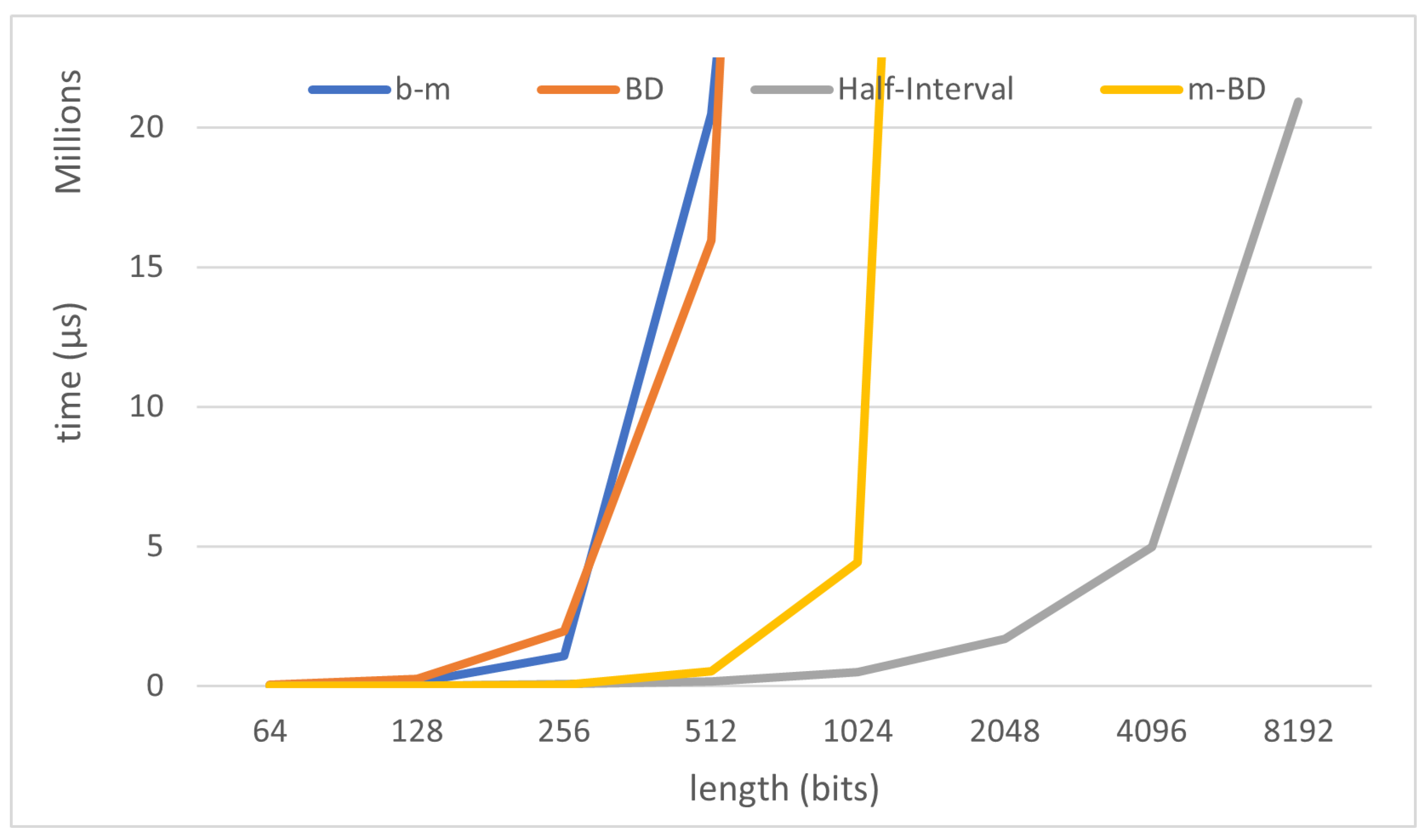
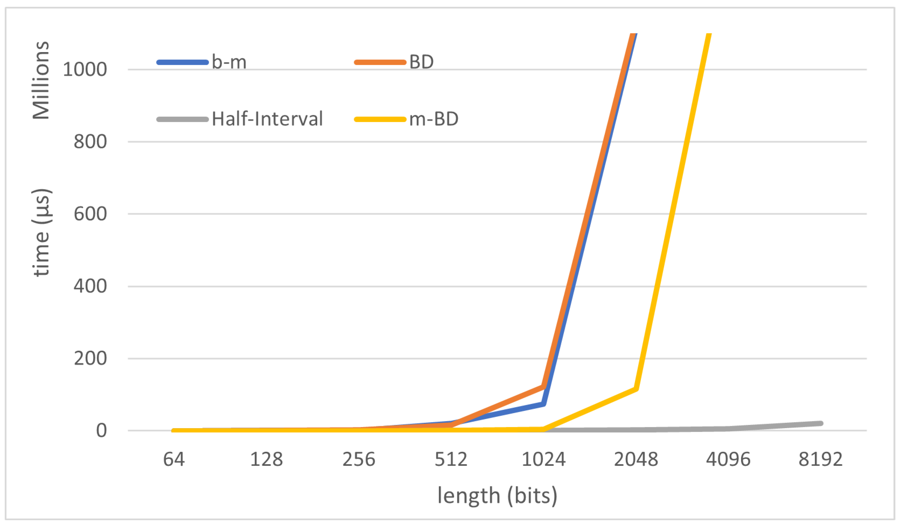
The results of the experiments can be seen in Figure 3 and Figure 4. Indeed, in Figure 3 where all algorithms are compared, we can see how as far as the length of the sequence increases, both the half-interval algorithm and the matrix binomial decomposition algorithm improve the performance exhibited by the Berlekamp-Massey algorithm. This proves that the binomial decomposition technique can be useful and a good alternative in the study of sequences that are particularly hard to be analyzed by the Berlekamp-Massey algorithm.

About the Berlekamp-Massey and the Binomial Decomposition algorithm, there is a bounce in their performance depending on the length of the sequences of the experiment. According to the study of the BD complexity, it is known that its performance depends on the parameter r, or in other words, it depends on the number of binomial sequences in the decomposition for each sequence. After the preliminary study on the parameter r, seen in Figure 2, the parameter r is expected to behave in a normal distribution fashion. Altogether this means that the BD algorithm can slightly change its performance depending on the r value of the sequences it is studying.

In addition, the theoretical improvement of the half-interval algorithm studied in the previous section is confirmed. The huge performance gap between Berlekamp-Massey algorithm, BD-algorithm, m-BD and the half-interval search algorithm can be seen in Figure 3 and Figure 5. Recall that this gap is particularly remarkable when the length of the sequence studied increases. For that reason we included Figure 3, scaled for a better comparison with the half-interval results (the best performant algorithm), and Figure 5, for a better comparison with m-BD (a novel contribution of this article).

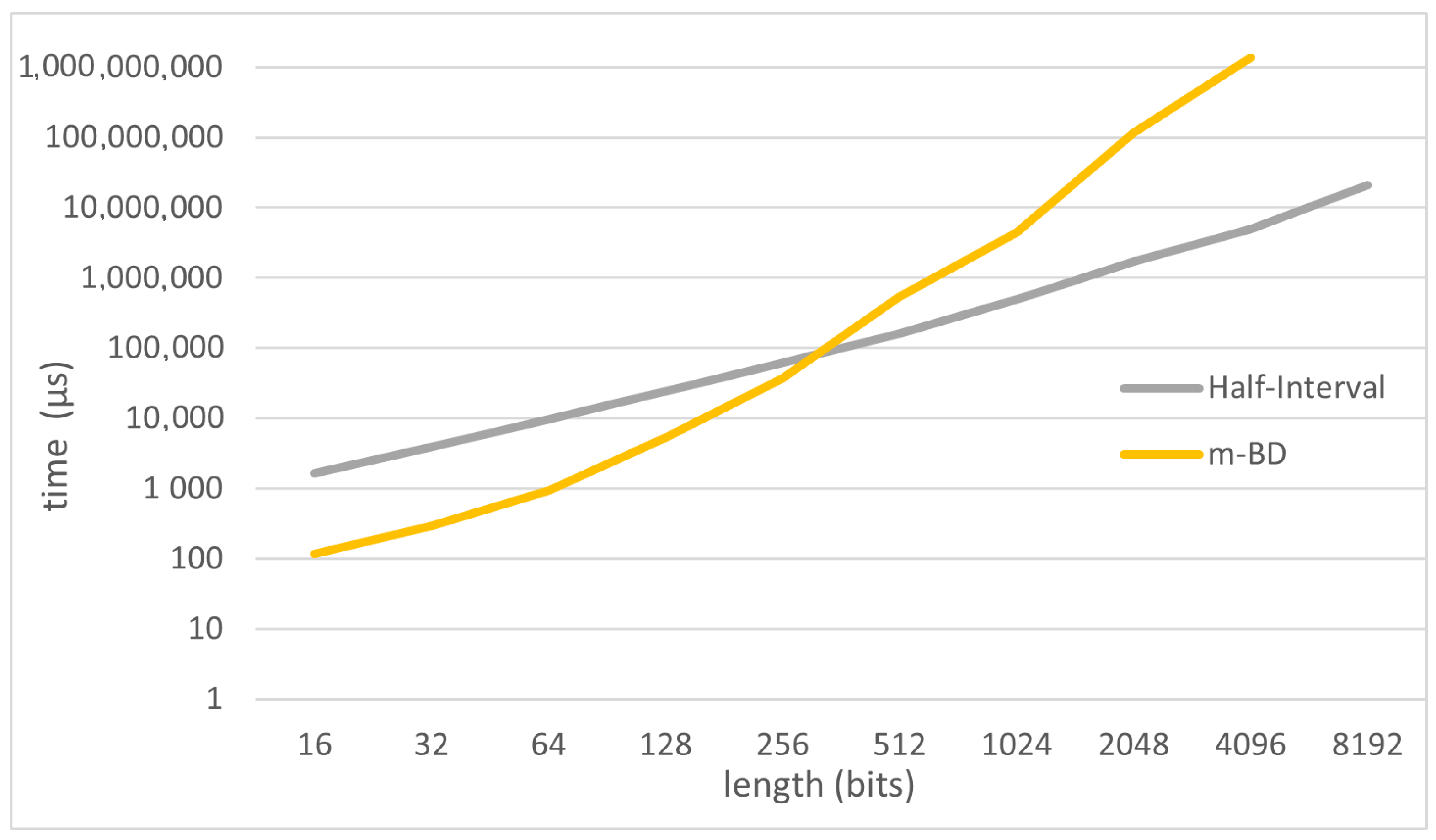
Furthermore, we wanted to compare the half-interval algorithm with the new m-BD algorithm, which has not been previously studied neither its performance is known. In Figure 4, a logarithmic scaled graph is depicted. We see how the half-interval search algorithm outperforms the m-BD algorithm provided that the length of the sequence studied is increased. This behaviour seems to reveal that the increment in the sequence length makes worse the m-BD algorithm performance, since m-BD requires more tries to calculate the $LC$.

Although it is not the purpose of this work, it is worth noticing that the half-interval search algorithm can be parallelized in the computation of $LC$ while the BD-algorithm performs the computation in a sequential way.

Another point that was not covered in the experiments is how the m-BD algorithm can take profit of some optimizations in the computation of matrix operations, which explain its great speed when the sequences are not too long. In addition, it could be enhanced while running in environments specially designed for it such as MATLAB.

5.3. Different Use-Cases

After the analysis and the experiments to test the performance of the algorithms, it is also worth exploring different application scenarios, not only the linear complexity calculation. All the algorithms that use the binomial decomposition calculate the $LC$ with the maximum binomial component.

A different case for these algorithms could be the study in depth of other types of binary sequences. In fact, having their full decomposition can help to analyze more parameters related to the security of the sequences, e.g., to calculate the density of components in the decomposition or the balancedness of such sequences. It is in this case where the BD-algorithm outperforms the others, since the way it calculates the $LC$ is by means of the computation of all the binomial components.

Another interesting use-case for these algorithms is, for instance, processing a large amount of sequences in order to discern as fast as possible which ones have better/worse security. In that case, the m-BD algorithm is the best one, because it can determine whether the highest binomial component is present in the binomial decomposition previously to complete the $LC$ calculation. So the m-BD algorithm may not be the fastest algorithm to calculate the $LC$ of a particular sequence but it may be used to quickly detect which sequence has a $LC$ lower than the others.

Finally, the m-BD algorithm could be of great use if the range of the linear complexity is known. In that case, this parameter would avoid unnecessary tries of the algorithm, which otherwise will profit from the matrix optimizations that modern libraries support.

6. Conclusions

In this work, different algorithms to compute the linear complexity of binary sequences were introduced and analyzed. In general, they exhibit better performances than the well-known Berlekamp-Massey algorithm when applied to sequences suitable for cryptography.

Concerning the half-interval search algorithm presented in this article, it shows excellent results in both computational complexity and amount of sequence required. It was also tested in comparison with other algorithms by applying it to GSS-sequences, showing an improved performance when the length of the sequences increases.

The matrix binomial decomposition algorithm showed a good performance with short sequences. Nevertheless, its main characteristic, i.e., the way in which it identifies the binomial components of a sequence, can be useful in other scenarios apart from the $LC$ calculation, e.g., to discern between a large amount of sequences which ones have a better complexity than the others.

Moreover, the binomial decomposition of binary sequences seems to be an innovative technique to extract information from a given sequence. In particular, the fractal character of the binomial sequences can be employed to calculate diverse parameters of a sequence without knowing the whole sequence.

In brief, the analysis of these algorithms is quite useful to find weaknesses in this type of binary sequences. Indeed, detecting such weaknesses in a cipher with practical applications could compromise the corresponding IoT device and, consequently, the services that rely on it.

References

- Chin, W.L.; Li, W.; Chen, H.H. Energy big data security threats in IoT-based smart grid communications. IEEE Commun. Mag. 2017, 55, 70–75. [Google Scholar] [CrossRef]
- Meyer, D.; Haase, J.; Eckert, M.; Klauer, B. New attack vectors for building automation and IoT. In Proceedings of the IECON 2017-43rd Annual Conference of the IEEE Industrial Electronics Society, Beijing, China, 29 October–1 November 2017; pp. 8126–8131. [Google Scholar]
- Gallegos-Segovia, P.L.; Bravo-Torres, J.F.; Argudo-Parra, J.J.; Sacoto-Cabrera, E.J.; Larios-Rosillo, V.M. Internet of things as an attack vector to critical infrastructures of cities. In Proceedings of the 2017 International Caribbean Conference on Devices, Circuits and Systems (ICCDCS), Cozumel, Mexico, 5–7 June 2017; pp. 117–120. [Google Scholar]
- Rouf, I. Security and Privacy Vulnerabilities of In-Car Wireless Networks: A Tire Pressure Monitoring System Case Study. In Proceedings of the USENIX Security Symposium, Washington, DC, USA, 11–13 August 2010; Volume 10. [Google Scholar]
- Cynthia, J.; Sultana, H.P.; Saroja, M.; Senthil, J. Security protocols for IoT. In Ubiquitous Computing and Computing Security of IoT; Springer: Berlin/Heidelberg, Germany, 2019; pp. 1–28. [Google Scholar]
- Mavromoustakis, C.X.; Mastorakis, G.; Batalla, J.M. Internet of Things (IoT) in 5G mobile technologies; Springer: Berlin/Heidelberg, Germany, 2016; Volume 8. [Google Scholar]
- NIST Lightweight Cryptography Project. Available online: https://csrc.nist.gov/Projects/Lightweight-Cryptography (accessed on 15 February 2021).
- McGinthy, J.M. Solutions for Internet of Things Security Challenges: Trust and Authentication. Ph.D. Thesis, Virginia Tech, Blacksburg, VI, USA, 2019. [Google Scholar]
- NIST Lightweight Cryptography Project Round 2 Candidates. Available online: https://csrc.nist.gov/Projects/lightweight-cryptography/round-2-candidates. (accessed on 15 February 2021).
- Dubrova, E.; Hell, M. Espresso: A stream cipher for 5G wireless communication systems. Cryptogr. Commun. 2017, 9, 273–289. [Google Scholar] [CrossRef] [Green Version]
- Massey, J. Shift-register synthesis and BCH decoding. IEEE Trans. Inf. Theory 1969, 15, 122–127. [Google Scholar] [CrossRef] [Green Version]
- Cardell, S.D.; Fúster-Sabater, A. Binomial Representation of Cryptographic Binary Sequences and Its Relation to Cellular Automata. Complexity 2019. [Google Scholar] [CrossRef] [Green Version]
- Chang, K.Y.; Lee, M.K.; Lee, H.R.; Hong, D.W.; Kang, J.S.; Cho, H.S.; Chung, K.I. Method and Apparatus for Generating Keystream. US Patent 7,587,046, 8 September 2009. [Google Scholar]
- Kang, Y.S.; Kim, H.W.; Chung, K.I. Apparatus and Method for Protecting RFID Data. US Patent 8,386,794, 17 February 2013. [Google Scholar]
- Falk, R.; Merli, D. Programmable Logic Device, Key Generation Circuit and Method for Providing Security Information. EP Patent 3146520, 11 May 2016. [Google Scholar]
- Martin-Navarro, J.L.; Fúster-Sabater, A. Folding-BSD Algorithm for Binary Sequence Decomposition. Computers 2020, 9, 100. [Google Scholar] [CrossRef]
- Cardell, S.D.; Climent, J.J.; Fúster-Sabater, A.; Requena, V. Representations of Generalized Self-Shrunken Sequences. Mathematics 2020, 8, 1006. [Google Scholar] [CrossRef]
- Golomb, S.W. Shift Register Sequences; Aegean Park Press: Walnut Creek, CA, USA, 1967. [Google Scholar]
- Menezes, A.J.; van Oorschot, P.C.; Vanstone, S.A. Handbook of Applied Cryptography; CRC Press: Boca Raton, FL, USA, 1996. [Google Scholar]
- Paar, C.; Pelzl, J. Understanding Cryptography; Springer: Berlin, Germany, 2010. [Google Scholar]
- Cardell, S.D.; Fúster-Sabater, A. The t-Modified self-shrinking generator. In International Conference on Computational Science (ICCS 2018); Springer: Berlin/Heidelberg, Germany, 2018; pp. 653–663. [Google Scholar]
- Cardell, S.D.; Fúster-Sabater, A. Cryptography with Shrinking Generators: Fundamentals and Applications of Keystream Sequence Generators Based on Irregular Decimation; Series: Briefs in Mathematics; Springer: Berlin/Heidelberg, Germany, 2019. [Google Scholar]
- Coppersmith, D.; Krawczyk, H.; Mansour, Y. The shrinking generator. In Annual International Cryptology Conference; Springer: Berlin/Heidelberg, Germany, 1993; pp. 22–39. [Google Scholar]
- Meier, W.; Staffelbach, O. The self-shrinking generator. In Communications and Cryptography; Springer: Berlin/Heidelberg, Germany, 1994; pp. 287–295. [Google Scholar]
- Hu, Y.; Xiao, G. Generalized self-shrinking generator. IEEE Trans. Inf. Theory 2004, 50, 714–719. [Google Scholar] [CrossRef]
- Mihaljevic, M.J. A faster cryptanalysis of the self-shrinking generator. In Proceedings of the Information Security and Privacy, First Australasian Conference, ACISP’96, Wollongong, Australia, 24–26 June 1996; Lecture Notes in Computer Science. Springer: Berlin/Heidelberg, Germany, 1996; Volume 1172, pp. 182–189. [Google Scholar] [CrossRef]
- Simpson, L.; Golic, J.D.; Dawson, E. A Probabilistic Correlation Attack on the Shrinking Generator. In Proceedings of the Information Security and Privacy, Third Australasian Conference, ACISP’98, Brisbane, Australia, 13–15 July 1998; Lecture Notes in Computer Science. Springer: Berlin/Heidelberg, Germany, 1998; Volume 1438, pp. 147–158. [Google Scholar] [CrossRef]
- Caballero, P.; Fúster-Sabater, A.; Pazo, M.E. New Attack Strategy for the Shrinking Generator. J. Res. Pract. Inf. Technol. 2009, 23, 171–180. [Google Scholar]
- Fúster-Sabater, A.; Pazo, M.E.; Caballero, P. A Simple Linearization of the Self-Shrinking Generator by Means of Linear Cellular Automata. Neural Netw. 2010, 23, 461–464. [Google Scholar] [CrossRef]
- Cardell, S.D.; Fúster-Sabater, A.; Ranea, A.H. Linearity in decimation-based generators: An improved cryptanalysis on the shrinking generator. Open Math. 2018, 16, 646–655. [Google Scholar] [CrossRef]
- Fúster-Sabater, A.; Cardell, S.D. Linear complexity of generalized sequences by comparison of PN-sequences. Rev. De La Real Acad. De Cienc. Exactas, Físicas Y Naturales. Ser. A. Matemáticas 2020, 114, 79. [Google Scholar] [CrossRef]
- Fúster-Sabater, A. Generation of cryptographic sequences by means of difference equations. Appl. Math. Inform. Sci. 2014, 8, 475–484. [Google Scholar] [CrossRef]
- Cusick, T.W.; Stanica, P. Cryptographic Boolean Functions and Applications; Academic Press: Cambridge, MA, USA, 2017. [Google Scholar]
- Martin-Navarro, J.L.; Fúster-Sabater, A. Folding-BSD Algorithm for Binary Sequence Decomposition. In International Conference on Computational Science and Its Applications (ICCSA 2020); Springer: Berlin/Heidelberg, Germany, 2020; pp. 345–359. [Google Scholar]