
Robust Stabilization of Interval Plants with Uncertain Time-Delay Using the Value Set Concept

 , , ,
, , ,  and
and 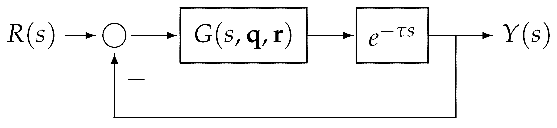
Abstract
:1. Introduction
2. Preliminaries and Problem Statement
2.1. Time-Delay Systems
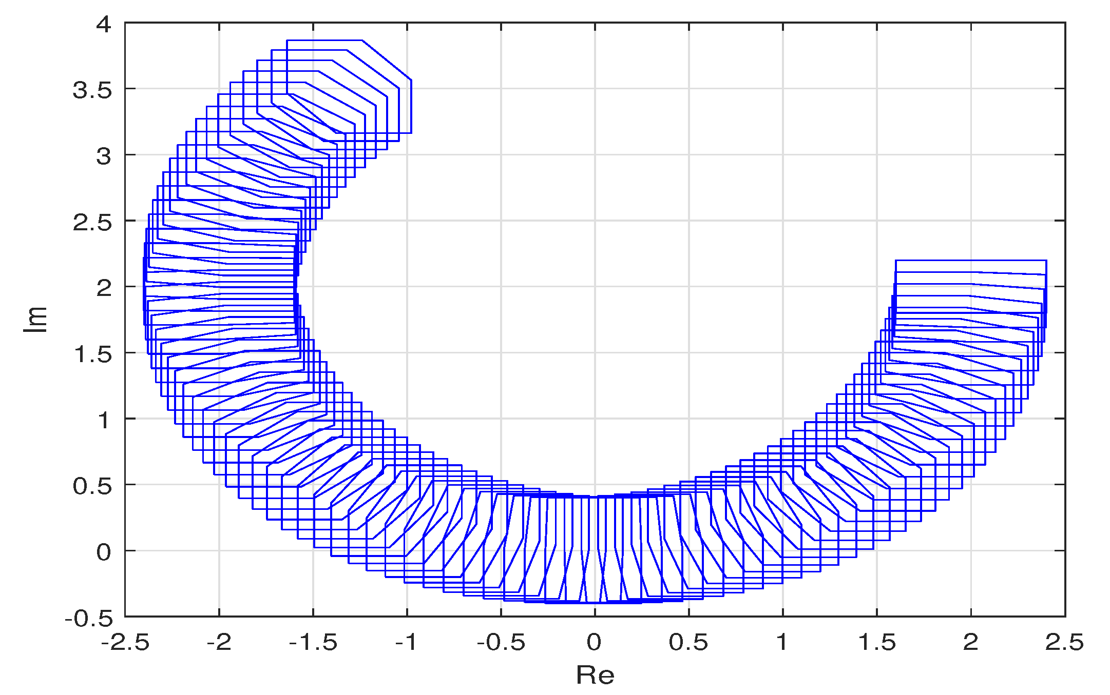
2.2. The Value Set
- Set as the corresponding value set associated with . is determined by the rotation radians clockwise about the origin of :Therefore, .
- Let be a nonnegative integer such that . If is not a multiple of , then is a polygon (parallelogram, hexagon, or octagon) with vertices inwhere, for , and , withOtherwise, is a rectangle with vertices in , . Here, the integer-valued function is defined as the remainder of m divided by 4.
- The geometric centers of , , and areandrespectively. Furthermore, the orbit of is an arc of a circle centered at with a radius equal to when τ increases, where stands for the modulus of the complex number z.
2.3. Orthogonal Polynomials on the Real Line
- if with , then and
- if with and , then .
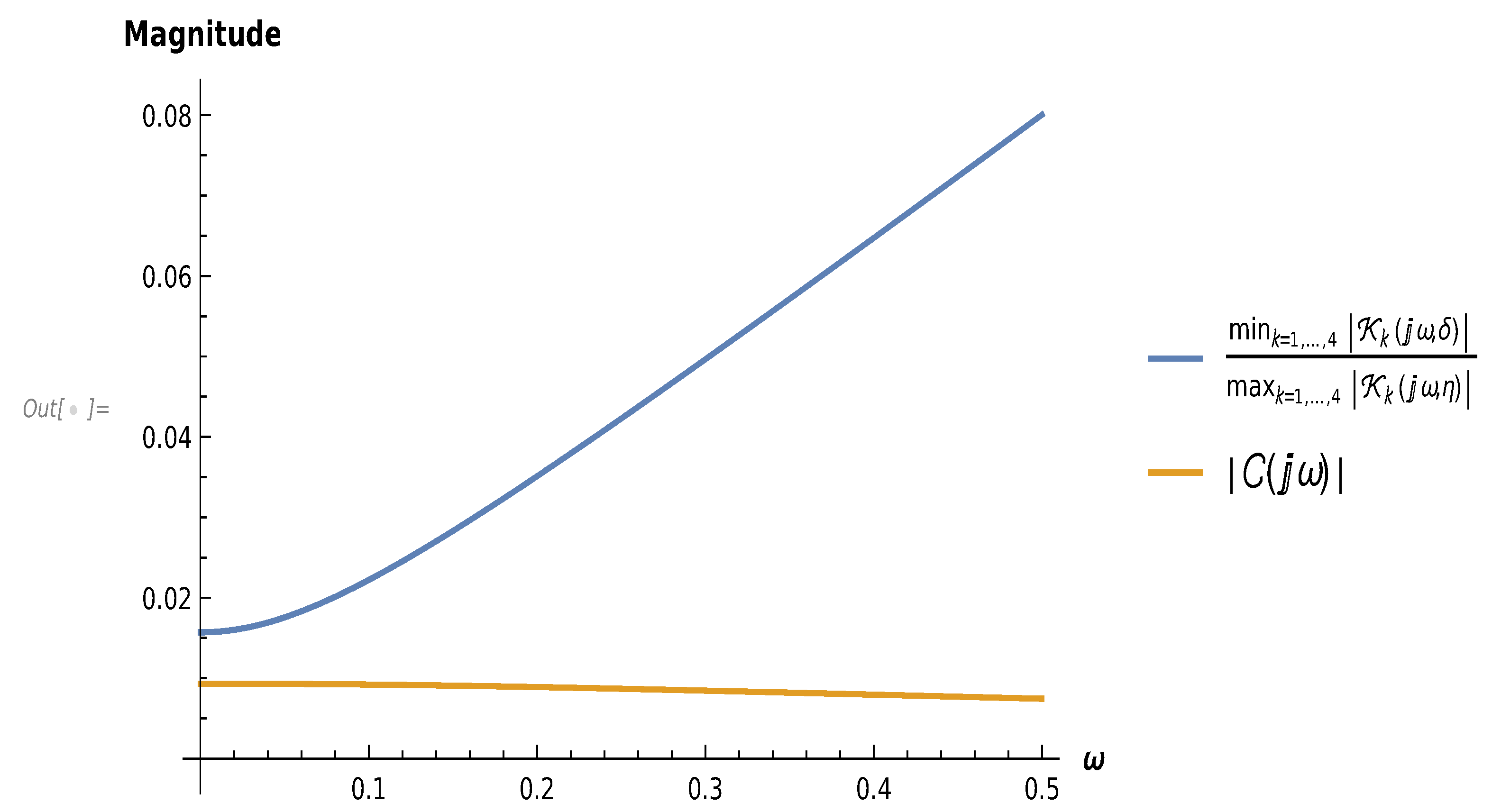
3. Results
- the orbits of each vertex of correspond to circular arcs centred on the vertices of with a radius equal to the modulus of every vertex of when τ increases, and
- for all , where .
- if , where and , and
- if .
3.1. Robust Stabilization of Interval Plants with a Time Delay
3.2. Compensators Associated with Modified Classical Weights
| Algorithm 1: Algorithm to select using modified classical orthogonal polynomials. |
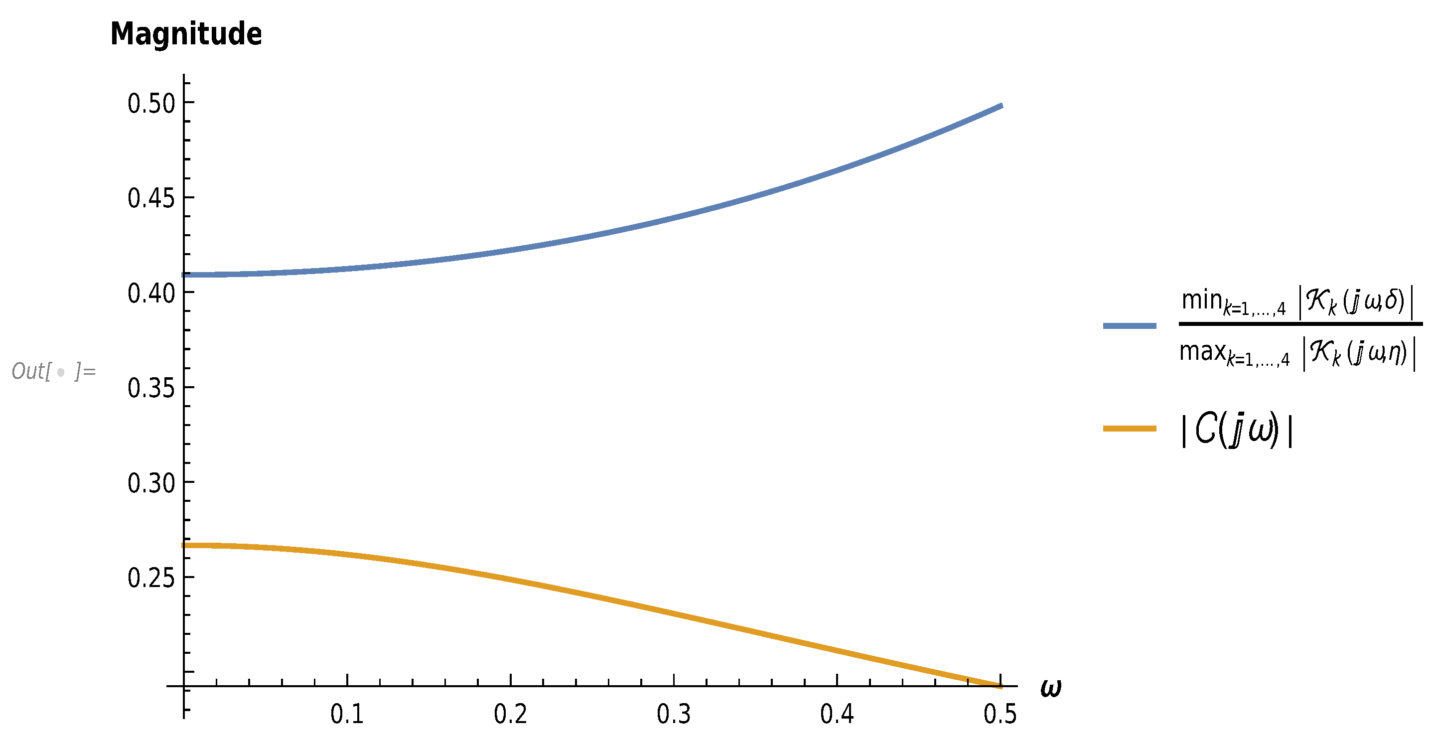
| Input: Any strictly proper interval plant satisfying the hypotheses of Theorem 2 and any positive integer m. Output: A strictly proper compensator with degree m such that the feedback structure shown in Figure 3 is robustly stable for all . Find such that for every ; find such that for every ; in the Laguerre case, select such that , where . In the Jacobi case, select , and such that , where ; compute and by using (6) and (7) (or (8) and (9)), respectively, with the selected values of and t (or , , and t); do . |
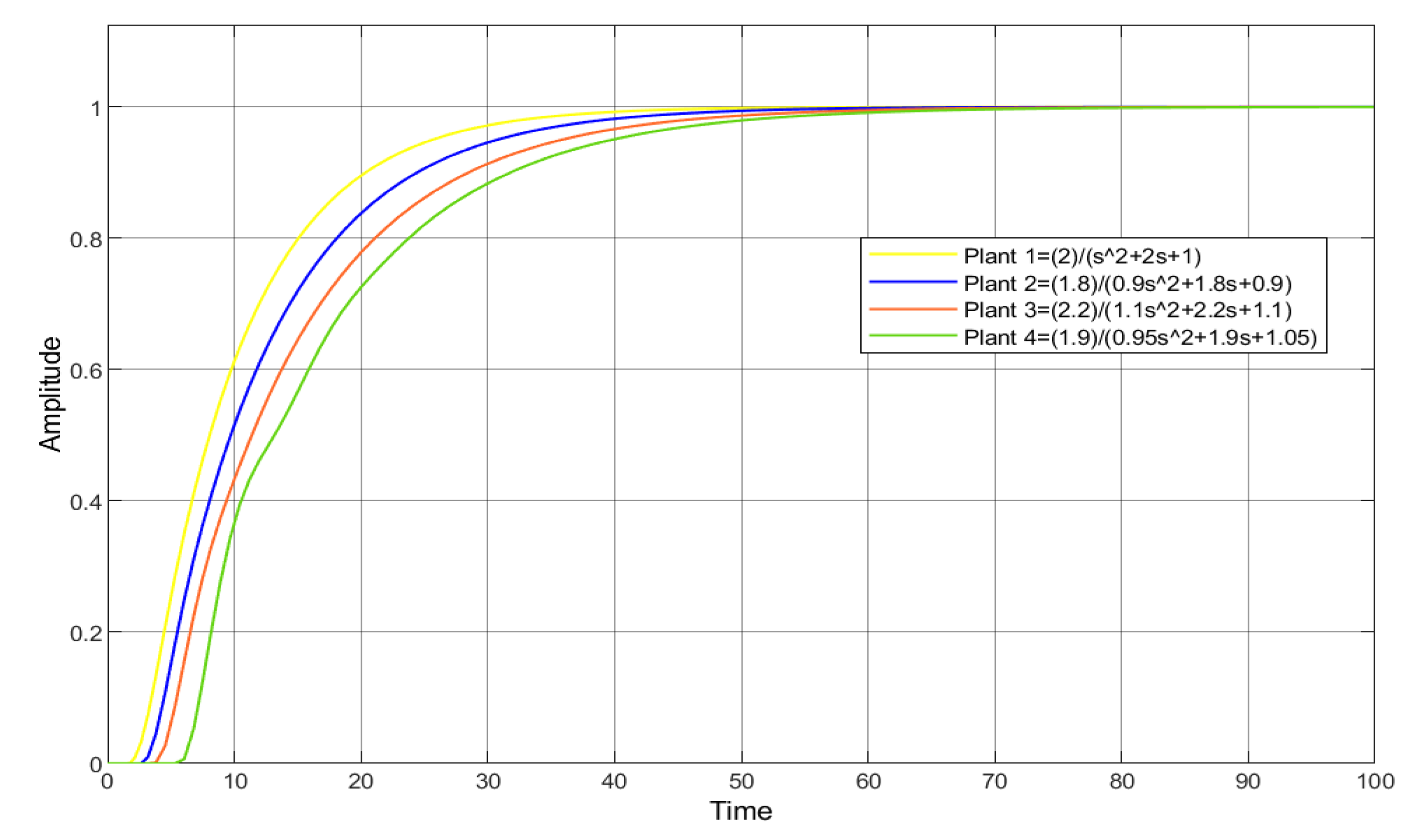
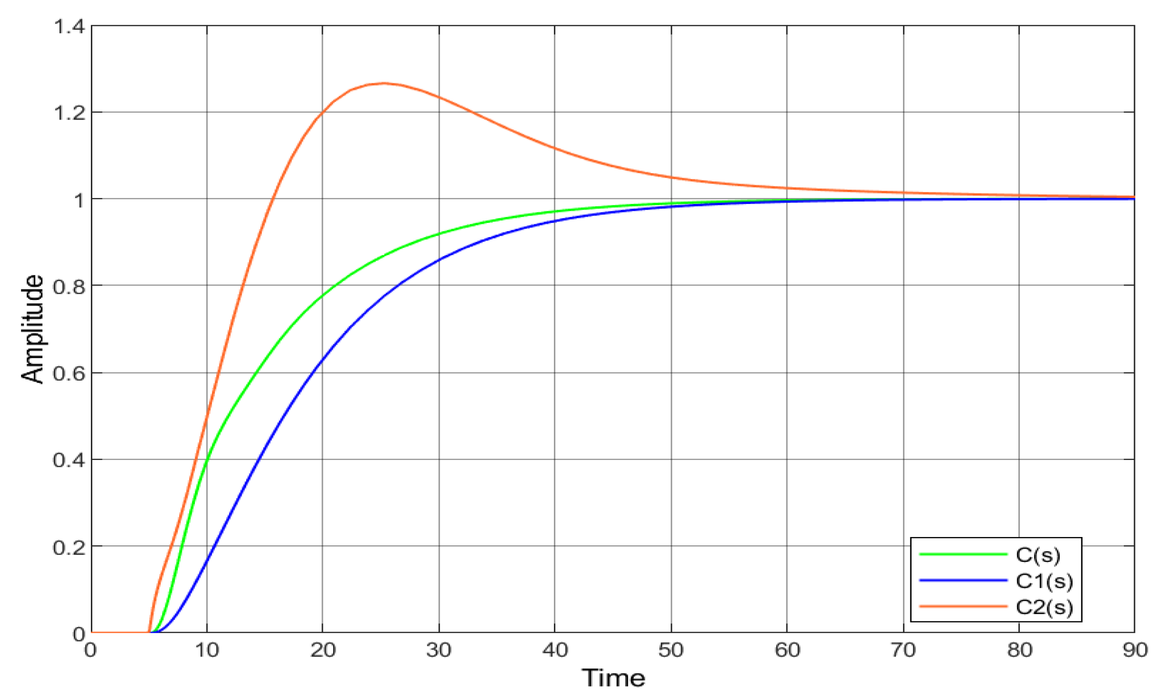
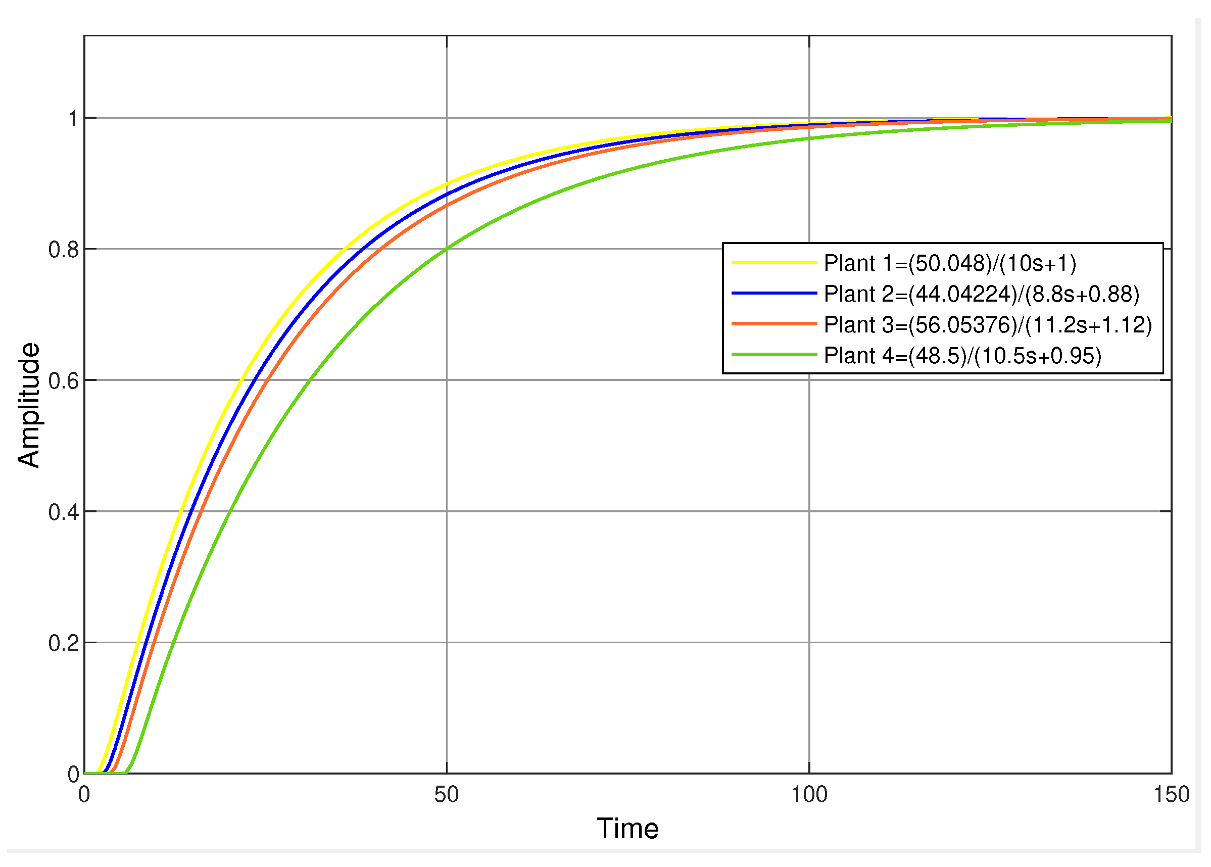
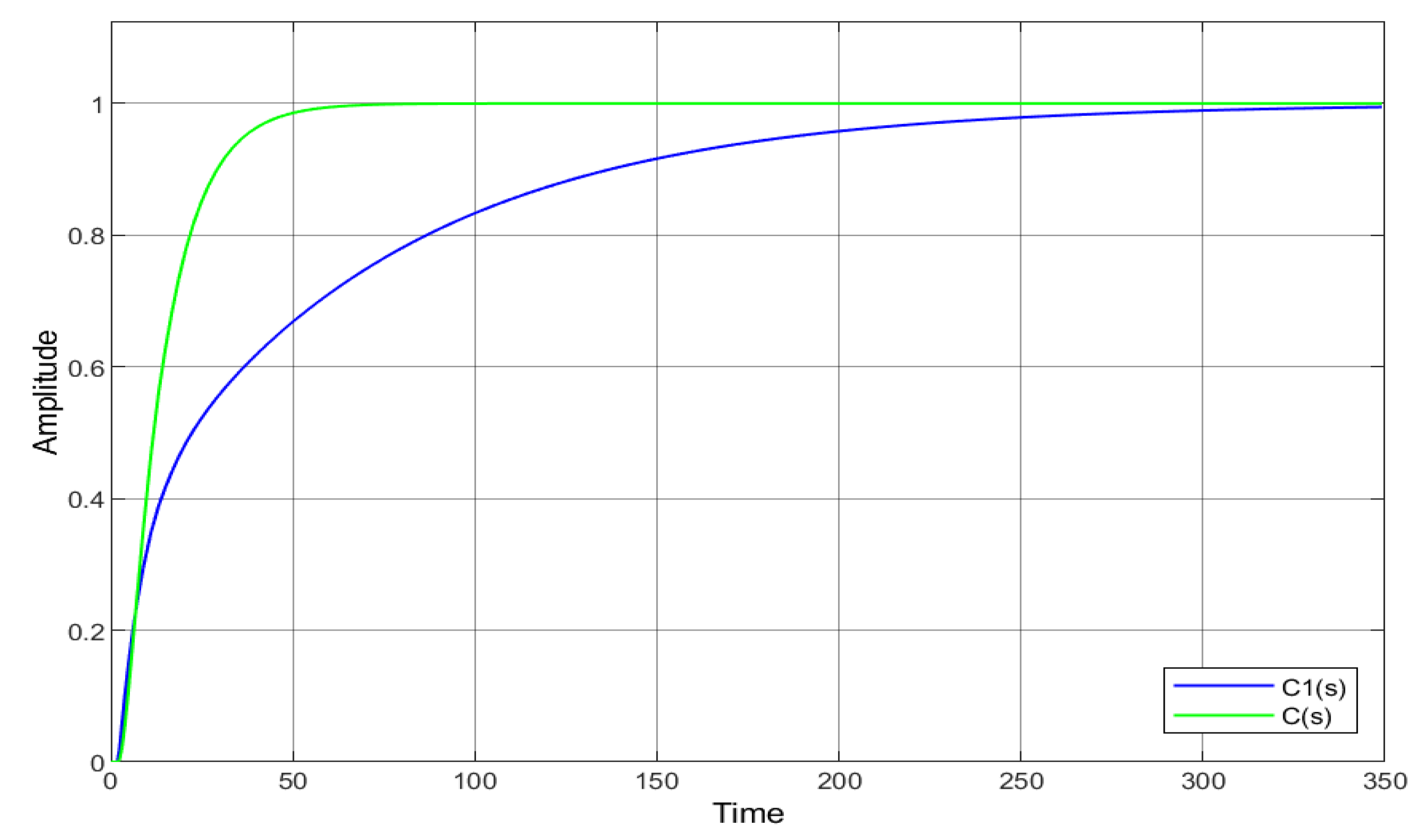
3.3. Simulation Results
- Find the reference value associated with the given plant, and propose a or a according to step 3 of Algorithm 1.
- Apply the designed controller to the examples, and validate the methodology through simulations.
4. Conclusions
5. New Directions
- The families of compensators considered in Algorithm 1 are constructed using some classical weights, given by Proposition 2. In order to obtain other families of compensators, we propose introducing some perturbations on the coefficients of the recurrence relation that orthogonal polynomials satisfy (see, for instance, [40]).
- In addition, it is possible to consider, in our problem, another type of parametric uncertainty structure such as affine linear, multilinear, and polynomic uncertainties (see [5]).
Author Contributions
Funding
Institutional Review Board Statement
Informed Consent Statement
Data Availability Statement
Acknowledgments
Conflicts of Interest
References
- Malek-Zavarei, M.; Jamshidi, M. Time-Delay Systems: Analysis, Optimization and Applications; North-Holland: Amsterdam, The Netherlands, 1987. [Google Scholar]
- Gu, K.; Niculescu, S. Survey on Recent Results in the Stability and Control of Time-Delay Systems. ASME J. Dyn. Syst. Meas. Control 2003, 125, 158–165. [Google Scholar] [CrossRef]
- Green, M.; Limebeer, D.J.N. Linear Robust Control; Prentice Hall: New York, NY, USA, 1995. [Google Scholar]
- Ackermann, J. Robust Control; Springer: London, UK, 1993. [Google Scholar]
- Barmish, B.R. New Tools for Robustness of Linear Systems; Macmillan Publishing Co.: New York, NY, USA, 1994. [Google Scholar]
- Wu, M.; He, Y.; She, J. Stability Analysis and Robust Control of Time Delay Systems; Springer: Beijing, China, 2010. [Google Scholar]
- Kharitonov, V.L. Robust Stability Analysis of Time Delay Systems: A Survey. IFAC Proc. Vol. 1998, 31, 1–12. [Google Scholar] [CrossRef]
- Papachristodoulou, A.; Peet, M.; Lall, S. Constructing Lyapunov-Krasovskii Functionals For Linear Time Delay Systems. In Proceedings of the 2005, American Control Conference, Portland, OR, USA, 8–10 June 2005; Volume 4, pp. 2845–2850. [Google Scholar]
- Seuret, A. Lyapunov-Krasovskii Functionals Parameterized with polynomials. IFAC Proc. Vol. 2009, 42, 214–219. [Google Scholar] [CrossRef] [Green Version]
- Duan, W.; Li, Y.; Chen, J. An enhanced stability criterion for linear time-delayed systems via new Lyapunov—Krasovskii functionals. Adv. Differ. Equ. 2020, 21. [Google Scholar] [CrossRef]
- Kharitonov, V.L. Asymptotic Stability of an Equilibrium Point Position of a Family of Systems of Linear Differential Equations. Plenum Publ. Corp. 1979, 1483–1485. [Google Scholar]
- Bartlett, A.C.; Hollot, C.V.; Lin, H. Root locations of an entire polytope of polynomials: It suffices to check the edges. Math. Control. Signals Sist. 1988, 1, 61–71. [Google Scholar] [CrossRef]
- Kalinina, E. Stability and D-stability of the family of real polynomials. Linear Algebra Appl. 2013, 438, 2635–2650. [Google Scholar] [CrossRef]
- Romero, G.; Zamora, P.; Díaz, I.; Pérez, I.; Lara, D. New Results to Verify the Robust Stability Property of Interval Plants with Time Delay. IFAC Proc. Vol. 2012, 45, 7–12. [Google Scholar] [CrossRef]
- Aguirre, B.; Villafuerte, R.; Luviano, A.; Loredo, C.; Díaz, E. A Panoramic Sketch about the Robust Stability of Time-Delay Systems and Its Applications. Complexity 2020, 2020, 1–26. [Google Scholar] [CrossRef]
- Manitius, A.; Olbrot, A. Finite Spectrum Assignment Problem for Systems with Delays. IEEE Trans. Autom. Control 1979, 24, 541–552. [Google Scholar] [CrossRef]
- Niculescu, S.L.; Dion, J.M.; Dugard, L. Robust stabilization for uncertain time-delay systems containing saturating actuators. IEEE Trans. Autom. Control 1996, 41, 742–747. [Google Scholar] [CrossRef]
- Mondie, S.; Michiels, W. Finite Spectrum Assignment of Unstable Time Delay Systems with a Safe Implementation. IEEE Trans. Autom. Control 2003, 48, 2207–2212. [Google Scholar] [CrossRef]
- Barmish, B.R.; Hollot, C.V.; Kraus, F.J.; Tempo, R. Extreme point results for robust stabilization of interval plants with first-order compensators. IEEE Trans. Autom. Control 1992, 37, 707–714. [Google Scholar] [CrossRef]
- Kharitonov, V.L.; Fu, M. Robust Synthesis of Time-Delay Systems. In Proceedings of the 32nd IEEE Conference on Decision and Control, San Antonio, TX, USA, 15–17 December 1993; pp. 326–327. [Google Scholar]
- Gao, Z. Robust stabilization of interval fractional-order plants with one time-delay by fractional-order controllers. J. Frankl. Inst. 2017, 354, 767–786. [Google Scholar] [CrossRef]
- Zheng, S.; Li, W. Robust stabilization of fractional-order plant with general interval uncertainties based on a graphical method. Int. J. Robust Nonlinear Control 2017, 28, 1672–1692. [Google Scholar] [CrossRef]
- Patre, B.M.; Deore, P.J. Robust stability and performance of interval process plant with interval time delay. Trans. Inst. Meas. Control 2011, 34, 627–634. [Google Scholar] [CrossRef]
- Matusu, R.; Senol, B.; Pekar, L. Robust PI Control of Interval Plants With Gain and Phase Margin Specifications: Application to a Continuous Stirred Tank Reactor. IEEE Access 2020, 8, 145372–145380. [Google Scholar] [CrossRef]
- Dasgupta, S. Kharitonov’s Theorem Revisited. Syst. Control Lett. 1988, 11, 381–384. [Google Scholar] [CrossRef]
- Romero, G.; Collado, J. Robust Stability of Interval Plants with Perturbed Time Delay. In Proceedings of the 1995 American Control Conference (ACC’95), Seattle, WA, USA, 21–23 June 1995; Volume 10, pp. 326–327. [Google Scholar]
- Chihara, T.S. An Introduction to Orthogonal Polynomials; Mathematics and its Applications Series 13; Gordon and Breach: New York, NY, USA, 1978. [Google Scholar]
- Ismail, M.E.H. Classical and Quantum Orthogonal Polynomials in One Variable. In Encyclopedia of Mathematics and Its Applications; Cambridge University Press: Cambridge/London, UK, 2005; Volume 98. [Google Scholar]
- Van Assche, W. Orthogonal polynomials, associated polynomials and functions of the second kind. J. Comput. Appl. Math. 1991, 37, 237–249. [Google Scholar] [CrossRef] [Green Version]
- Bochner, M. Über Sturm—Liouvillesche polynomsysteme. Math. Zeit. 1929, 29, 730–736. [Google Scholar] [CrossRef]
- Branquinho, A.; Marcellán, F.; Petronilho, J. Classical orthogonal polynomials: A functional approach. Acta Appl. Math. 1994, 34, 283–303. [Google Scholar]
- Szegö, G. Orthogonal Polynomials, 4th ed.; American Mathematical Society Colloquium Publications Series; American Mathematical Society: Providence, RI, USA, 1975; Volume 23. [Google Scholar]
- Arceo, A.; Garza, L.E.; Romero, G. Robust stability of hurwitz polynomials associated with modified classical weights. Mathematics 2019, 7, 818. [Google Scholar] [CrossRef] [Green Version]
- Andrews, G.; Askey, R.; Roy, R. Special Functions. In Encyclopedia of Mathematics and its Applications; Cambridge University Press: Cambridge/London, UK, 1999. [Google Scholar]
- Webster, R. Convexity, 3rd ed.; Oxford University Press: New York, NY, USA, 1994. [Google Scholar]
- Dlapa, M. Parametric uncertainties and time delay robust control design toolbox. IFAC-Papers Online 2015, 48, 296–301. [Google Scholar] [CrossRef]
- Romero, G.; Garcia, L.; Perez, I.; Dominguez, R.; Panduro, M.; Mendez, A. Robust Stability of the Hot-Dip Galvanizing Control Systems. Int. J. Autom. Control 2007, 1, 220–232. [Google Scholar] [CrossRef]
- Åström, K.J.; Wittenmark, B. Computer-Controller Systems: Theory and Design. In Prentice Hall Information and System Sciences, 3rd ed.; Prentice Hall Inc.: Upper Saddle River, NJ, USA, 1997. [Google Scholar]
- Chen, C.-T. Linear Systems: Theory and Design. In Electrical and Computer Engineering, 3rd ed.; Oxford University Press Inc.: New York, NY, USA, 1999. [Google Scholar]
- Marcellán, F.; Dehesa, J.S.; Ronveaux, A. On orthogonal polynomials with perturbed recurrence relations. J. Comput. Appl. Math. 1990, 30, 203–212. [Google Scholar] [CrossRef] [Green Version]


Publisher’s Note: MDPI stays neutral with regard to jurisdictional claims in published maps and institutional affiliations. |
© 2021 by the authors. Licensee MDPI, Basel, Switzerland. This article is an open access article distributed under the terms and conditions of the Creative Commons Attribution (CC BY) license (http://creativecommons.org/licenses/by/4.0/).
Share and Cite
Zamora, P.; Arceo, A.; Martínez, N.; Romero, G.; Garza, L.E. Robust Stabilization of Interval Plants with Uncertain Time-Delay Using the Value Set Concept. Mathematics 2021, 9, 429. https://doi.org/10.3390/math9040429
Zamora P, Arceo A, Martínez N, Romero G, Garza LE. Robust Stabilization of Interval Plants with Uncertain Time-Delay Using the Value Set Concept. Mathematics. 2021; 9(4):429. https://doi.org/10.3390/math9040429
Chicago/Turabian StyleZamora, Pedro, Alejandro Arceo, Noé Martínez, Gerardo Romero, and Luis E. Garza. 2021. "Robust Stabilization of Interval Plants with Uncertain Time-Delay Using the Value Set Concept" Mathematics 9, no. 4: 429. https://doi.org/10.3390/math9040429