1. Introduction
The functioning of Coriolis vibratory gyroscopes (CVG) is based on the effect of the precession of elastic waves excited in axisymmetric shells [
1,
2,
3]. Taking into account the fact that the main part of the vibration energy of the elastic shell corresponds to the region adjacent to its edge, the ring-shaped model is the basic one for studying the dynamics of the CVG of any configuration.
It is especially simple to analyze the dynamics of a ring-shaped CVG resonator in the case of a constant angular rate. With certain dependencies, by reducing to the known second-order differential equations with variable coefficients, the solutions of the equations of dynamics can also be found analytically [
4]. However, firstly, the form of these solutions can be quite cumbersome (expressed in terms of special functions). Secondly, not every law of rotation of the base allows one to obtain well-studied analytically differential equations. In particular, this applies to such practically important cases when the analytical dependence changes smoothly or abruptly with time, as well as if it is specified not in analytical but in tabular form.
Therefore, the numerical methods of solution are the most universal [
5]. One of the most significant drawbacks of numerical methods is the need to find a compromise between the speed and accuracy of difference schemes. It is not possible to obtain a solution at some time moment without evaluation of the solutions at all previous time grid knots. To construct a continuous solution by the discrete set of values, additional approximation is required. Finally, it is almost impossible to get physical interpretation of the numerical solutions obtained by means of the finite difference method.
To preserve the advantages of analytical methods, which make it possible to quickly calculate the parameters of motion at any predetermined moment of time according to given initial conditions, and at the same time use the universality of numerical methods, the following numerical–analytical approach is proposed in this work. Its essence lies in the piecewise approximation of an arbitrary dependence with the subsequent exact solution of problems on each elementary segment. In this case, it is enough just to calculate the values of the linear displacement and acceleration of the points of the ring at the end of a subinterval, which are at the same time the initial conditions for the subsequent segment. In this paper, we first consider the simplest piecewise constant approximation of the angular rate. Then we move on to consider the piecewise linear approximation of an arbitrary angular rate, based on the analytical solution for a linear angular velocity on each subinterval, taking into account situations requiring the use of asymptotic expansions. The latter are important in the case of high-intensity dynamics of CVG [
6,
7]. In the experimental section, we compare both types of solution and show the benefits of the piecewise linear approximation.
2. Statement of the Problem
Unlike the variety of microelectromechanical systems (MEMS) designs based on lumped masses for sensing Coriolis acceleration [
3], the ring-shaped CVG [
8,
9,
10], as well as the hemispherical resonator gyroscope (HRG) [
2] or the cylindrical resonator gyroscope (CRG) [
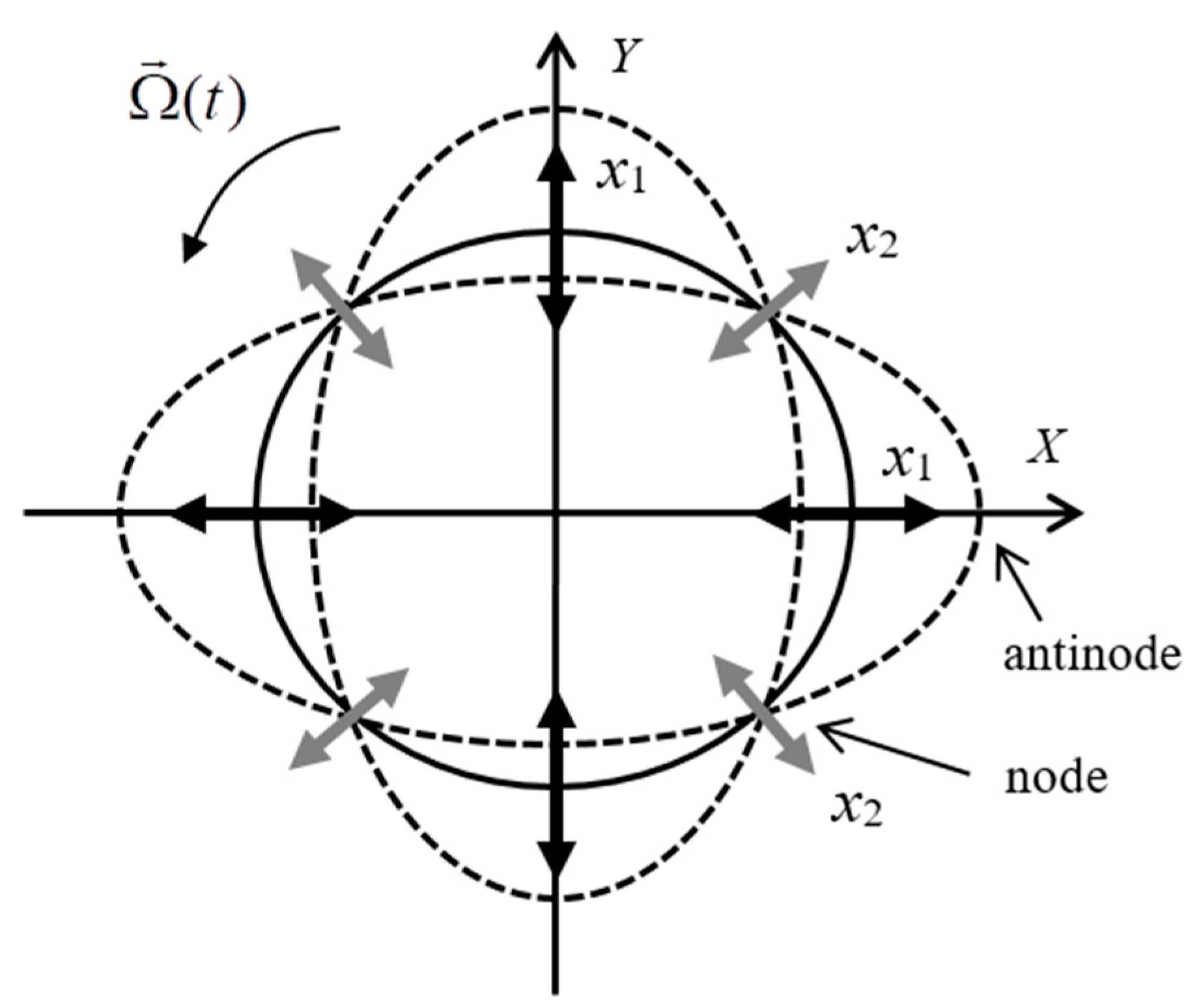
11], are examples of devices using sensitive elements with distributed masses. An in-plane standing wave is excited in an elastic ring-shaped resonator oscillating along axes
X and
Y with primary displacement
(
Figure 1). In the absence of external rotation applied to the resonator, the primary wave has four nodes with zero ring displacement, which are located at 45 deg between axes
X and
Y. After applying a rotation
around the sensitive axis, perpendicular to the plane of the ring, the primary wave begins to move around the ring due to the effect of the Coriolis inertia forces. As a result of this movement, secondary oscillations appear at the node points, thus making it possible to measure external angular rate projection to the sensitivity axis
. This phenomenon of standing wave inertia in rotating axisymmetrical solid bodies was first observed by G. Bryan [
12] and sometimes is called the Bryan effect.
In dimensionless form, the system of motion equations for free oscillations of such perfect ring-shaped CVG without dissipation can be written as [
3]
where
and
are the primary and secondary displacements;
is the natural frequency;
is the angular rate projection; and
is the CVG’s coupling factor (the Bryan coefficient) corresponding to the excited mode of oscillations.
To obtain the unique solution to Equation (1), the initial conditions at time moment
must be given:
Unlike a number of other works, in Equation (1) we do not assume that and/or . Instead, we will solve Equation (1) taking into account both the centrifugal forces corresponding to terms and the variable angular rate .
In the matrix form, Equation (1) can be written as
where
According to [
13], we introduce a variable phase
and change the variables as
or
Obviously,
and
where
I is the identity matrix.
Substituting Equation (8) in Equation (3), after left multiplication by matrix
, we get
Assuming
we obtain the system of ordinary differential equations (ODEs)
which can be solved independently for each scalar function
.
In previous works, researchers usually supposed that
and neglect the second term in square brackets in Equation (11) even if the angular rate is not constant [
3]. In this case, the solution of Equation (11) is simple and obtained in the form of trigonometric functions. However, if we need to study high-intensive dynamic processes with variable angular rates [
5,
6], we cannot omit the term
and must solve ODE (11) with a variable coefficient.
Considering that
initial conditions for the new variables will take the form
In particular, for the most important second form of in-plane oscillations with four nodes and four antinodes (
Figure 1), the angle between the axes of secondary displacements,
and
, is equal to
, and we have
,
.
Each ODE of system (11) takes the form
It should be noted that for the HRG, CRG, or other CVG models it is possible to obtain movement equations analogous to Equation (11), but with corresponding coefficients before the term .
The ODE (14) can be easily solved exactly for the case of a constant angular rate. If the angular rate is variable, it is possible to make its rough piecewise constant (stepwise) approximation with recurrent redefinition of initial conditions (13). This idea is explained in the next section.
3. Stepwise Approximation
In the case of
, Equation (14) has two linearly independent solutions
The variable phase (10) is equal to
The solution to Equation (14) has the form
with undetermined coefficients
found from initial conditions (13).
Let the angular rate
be defined on interval
. Introduce the uniform mesh
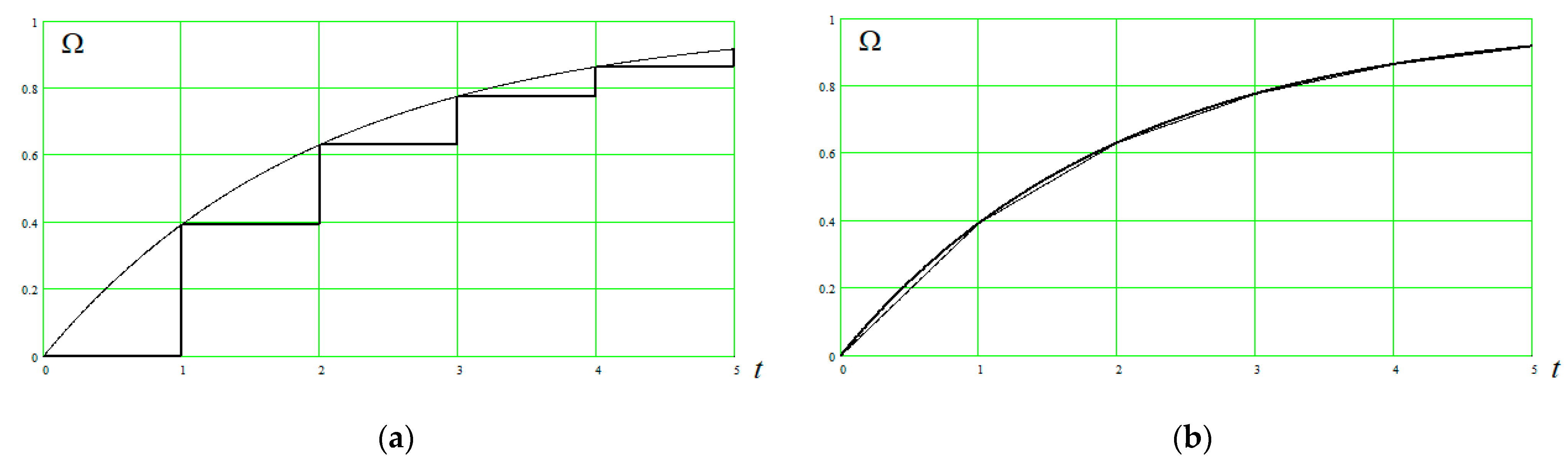
The stepwise approximation of
is expressed in the following way:
where
are the zero-order B-splines [
14].
On each interval
, we have
The general algorithm is to recursively obtain a solution of ODE (14) with constant angular rate (21) on each of subintervals . On the start subinterval , the initial conditions (13) are used, and to determine the initial conditions on each subinterval , , it is necessary to use the values calculated on the previous subinterval .
Instead of coefficients in Equation (19), one can take other values providing slightly better accuracy in different metrics, for example, . However, the order of approximation accuracy here remains the same, i.e., .
4. Piecewise Linear Approximation
Unfortunately, the stepwise approximation (19) having the 1st order of accuracy with respect to the time step h is not sufficient for precise and fast measurements. Therefore, the high-order representations of should be used, for example, the piecewise linear approximation having the 2nd order of accuracy with respect to h.
The main difficulty in using the piecewise linear approximation is in the fact that in previous works researchers did not study analytically the case of linear angular rate. In addition to the trivial case of the constant angular rate considered in
Section 3, one can also find the analytical solutions for the cases of angular rate changing according to the parabolic law (in the form of the Bessel functions) and the harmonic and poly-harmonic laws (in the form of Mathieu functions) [
4].
In this regard, we will further consider in more detail the solution for the case of a linear angular rate
Substituting Equation (22) in Equation (14), we obtain
Using a linear change of variable, we reduce Equation (23) to the standard form of the Weber equation for parabolic cylinder functions with respect to the new variable
[
15]:
where
Even and odd linearly independent solutions to Equation (24) have the form
where
At large times (
) or at small angular rate values (
), it is necessary to keep a sufficiently large number of terms of strongly oscillating infinite power series (25). In this regard, a variety of asymptotic representations should be used. In most cases of practical importance, the Darwin expansions [
15] are suitable fast enough representations. For example, if
is large and negative and
is moderate, we can take
where
Some of the first coefficients
are given by
The variable phase (10) is equal to
Now we apply the piecewise linear approximation of arbitrary
on the regular mesh (18):
where the linear B-splines are [
13]
It can be seen that for
where
The common piecewise linear approximation algorithm is analogous to that for the stepwise approximation considered in
Section 3.
Obviously, if the dependence of the angular rate is initially piecewise linear, then it is possible to obtain an exact solution through the Weber functions by appropriately choosing a non-uniform approximation grid. In this case, on subintervals
with
, we use the simplest analytical solutions (17) expressed in terms of trigonometric functions (15) and on subintervals with nonzero angular acceleration we apply the representation (17) expressed, depending on the sign of the acceleration and its absolute value as well as the length of the time interval, in terms of power series (25), Darwin expansions (26), or other asymptotic expansions [
15].
5. Numerical Experiment
As an example we will find the solution to Equation (1) on interval
, with an angular rate increasing according to the law [
7]:
We take the following boundary conditions (2):
Two types of approximations on the grid with
(grid width
) are shown on
Figure 2.
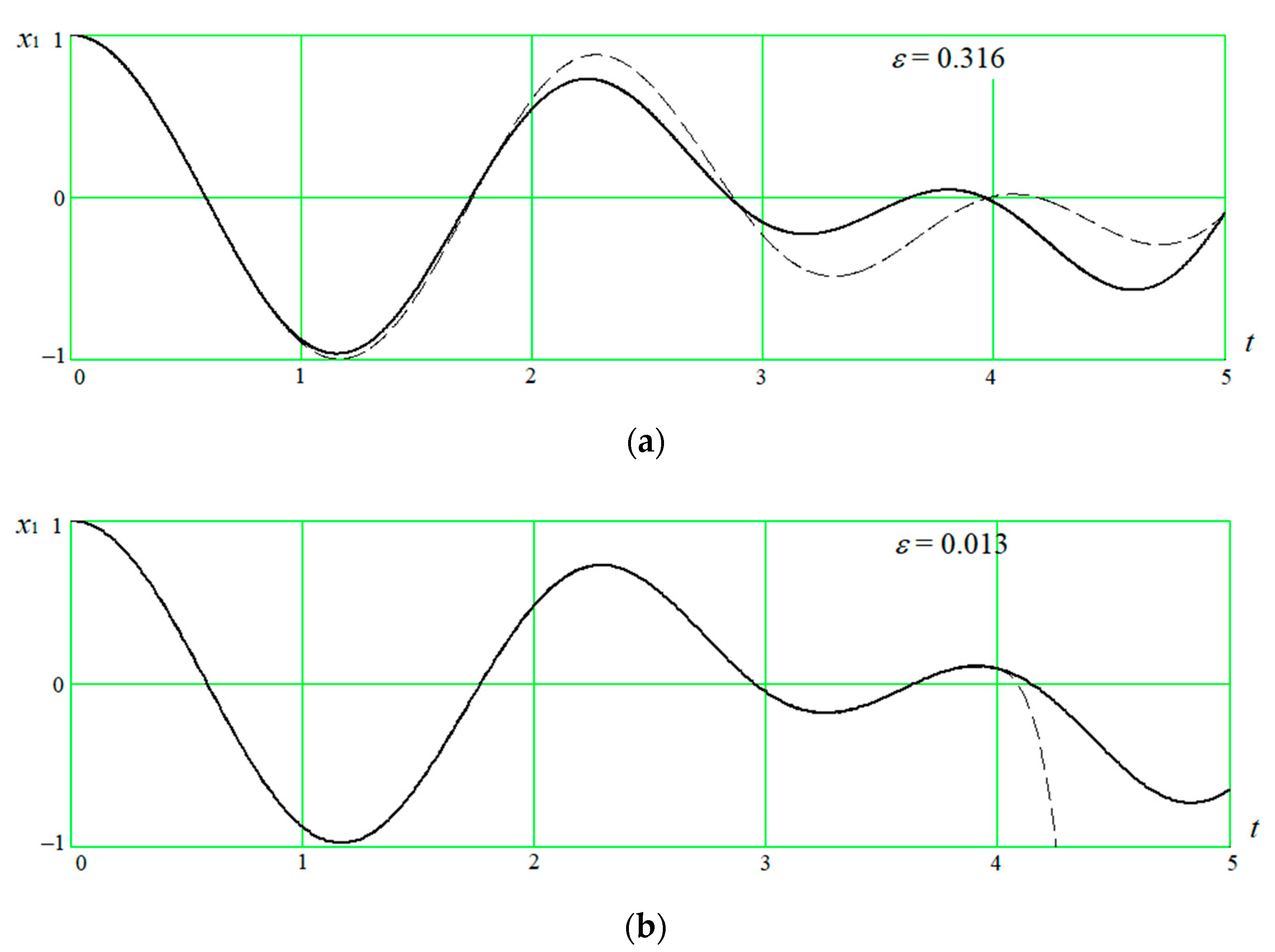
On
Figure 3 the dynamics of the primary displacement
is shown, evaluated by different approaches. The results were compared with solution
(bold line) obtained by the high-order finite-difference procedure on the dense grid with width
[
7]. Relative errors were computed according to the formula
It is seen that the piecewise linear approximation with Darwin representation provides much better accuracy () in comparison with the stepwise representation (). In turn, it should be noted that the piecewise representation in the form of power series (25) is accurate only on relatively short time intervals and demonstrates instability at . Moreover, the latter approach is also much more computationally expensive (the number of terms in time series was 40) in comparison with the Darwin asymptotic expressions (26).
This example demonstrates the benefits of the novel approach based on linear piecewise approximation of an angular rate in comparison with rough method of stepwise approximation. We must mention that although analytical solutions obtained earlier for angular rates changing according to parabolic and harmonic laws [
4] can also be applied for constructing the solution for arbitrary angular rate profiles, they require the use of more complicated approximation tools: parabolic B-splines and Fourier series, respectively. In the latter case it is difficult to approximate the non-smooth angular rate dynamics due to the necessity to take a large number of terms and the Gibbs effect. Taking these considerations into account we can conclude that the best way to arbitrary CVG’s dynamics simulation is the combination of both approaches proposed in our work (stepwise and linear piecewise), depending on the behavior of the angular rate.


