High-Performance Tracking for Piezoelectric Actuators Using Super-Twisting Algorithm Based on Artificial Neural Networks

Abstract

Piezoelectric actuators (PEA) are frequently employed in applications where nano-Micr-odisplacement is required because of their high-precision performance. However, the positioning is affected substantially by the hysteresis which resembles in an nonlinear effect. In addition, hysteresis mathematical models own deficiencies that can influence on the reference following performance. The objective of this study was to enhance the tracking accuracy of a commercial PEA stack actuator with the implementation of a novel approach which consists in the use of a Super-Twisting Algorithm (STA) combined with artificial neural networks (ANN). A Lyapunov stability proof is bestowed to explain the theoretical solution. Experimental results of the proposed method were compared with a proportional-integral-derivative (PID) controller. The outcomes in a real PEA reported that the novel structure is stable as it was proved theoretically, and the experiments provided a significant error reduction in contrast with the PID.

1. Introduction

In the early 1970s, the high accuracy positioning was constrained only at academic domains; however, as a result of advanced fabrication methods, the beginning of the current century leads the possibility of bringing micro-actuators in industrial environments [1]. Piezoelectric actuators (PEAs) are suitable candidates when there is an application that needs for nano-microdisplacement combined with precision as requirements [2]. Additionally, these systems provide accuracy and mechanical capabilities due to their high stiffness [3]. The blend is produced with the advantage of their size, which is an asset for the downsizing trend in actuators today. Due to these benefits, the applications are broad which includes energy harvesting [4], active vibration [5], motor design [6], etc. Furthermore, in recent years, the PEA has been a research aim for medical uses, such as drug delivery systems [7], micro grippers [8], spinal injection device [9], and orthodontic treatment [10].

The performance of these actuators downgrades due undesirable effects present in piezoelectric materials where the common ones are creep [11], vibration dynamics [12], and hysteresis. The latter is one of the most important and studied since the error can be up to 22% [13], which is a significant value when high precision is required in guidance systems. Furthermore, this phenomenon cannot be disregarded since not only affects a desired position but also it can yield the system to the instability [14].

The hysteresis is reflected as nonlinearity where the present input depends on the past values and usually is also defined as an effect that appears as a combination of mechanical strain and electric field [15,16]. Figure 1 is a figurative description at a material level when an electric field is applied through a piezoelectric material. In a neutral state without any electric action, the poles are in a arbitrary direction but when it gets exited, the poles begin to be aligned with the field, and an elongation is produced which is associated with the ferroelectric effect [17]. When the electric field decreases its value, the poles intention is to be back to their initial direction but with a certain difference compared to the one when the electric field started to increase its value and this produces the hysteresis [18].

According to Reference [19], there are two paths for hysteresis reduction: in terms of the raw matter, the piezoelectric material can be conceived up to an atomic level, which represents a complex task; at a practical level, a control strategy can be designed to drive the position to the desired one by controlling the voltage input signal.

As a first approach, linear controllers can be a suitable option to control the trajectory. In the early 1980s, authors of Reference [20] suggested to implement linear strategies to diminish hysteresis from PEAs. Although proportional-integral-derivative (PID) is a classic and simple integration tool for most applications, widely attractive works have been done in recent years [21,22,23]. Other PID variants had shown the inclusion of feedback linearization [24], grey relational [25], semiautomatic tuning [26], fractional PID [27], or gain-scheduling in a fuzzy-PID structure [28]. Besides, other authors had employed linear quadratic regulator for similar actuator in terms of structural control [29]. However, the hysteresis is a strong nonlinear effect where common structures need to have an advance design so as to diminish [30]. Moreover, with critical uncertainties, like modeling and external loads, these linear approaches are limited in a certain bandwidth [31].

The significant presence of nonlinearities in PEAs aims to implement controllers which can deal with these features. Feedback linearization with uncertainties control has been employed recently with the addition of a Bouc-Wen (BW) model for hysteresis where the researchers achieved good accuracy although the BW is limited for asymmetric hysteresis response [32,33]. An advance approach has equally been used with model predictive control based on an adaptive algorithm that was tested in a real system that provided an error of around 1%, which is an acceptable although tests were performed with low amplitude signals [34]. Robust controllers had also been investigated with adequate results; authors from Reference [35] implemented a robust control with its stability analysis of a scheme based on inverse models that produced decent outcomes as an error around 0.5 μm. In addition, other robust techniques as sliding mode control (SMC) had captured the interest due to its capability to reject the uncertainties [36,37]. Several approaches of first order SMC had been designed and used for PEAs, even though the chattering is an important drawback [38,39,40].

In recent years, many methods have been designed to overcome the chattering phenomenon [41,42,43,44]. Thus, the authors of References [41,42] implemented the boundary layer technique which changes the discontinuous term of SMC by a smooth approximation when the states are about to reach the limits of a defined bound; however, the main drawback of this method is the decline of anti-disturbance capabilities [45]. In Reference [43], a multi-surfaces SMC for approximation of unknown perturbations was proposed; despite the novelty of the framework, only simulation results were presented, and the algorithm has a broad number of gains for tuning. Integral Sliding Mode Control (ISMC) represents another employed structure for static-error reduction as it was developed in Reference [44]; nevertheless, when a saturation function is used, the practicality is reduced because the boundaries are complex to obtain and the control accuracy is diminished [46].

Another advanced method for chattering reduction is High Order Sliding Mode Control (HOSMC) that was introduced by Reference [47], which intention is to influence the high order derivatives of the system for the chattering alleviation. This technique is well known for its usage in Maximum Power Point Tracking (MPPT) control [48,49], active vehicle suspension [50], but it is also employed for high performance guidance in aircrafts [51] as in PEAs [52,53,54]. The Super-Twisting Algorithm (STA) belongs to the group of HOSMC and it is well known for its robustness and chattering decrease due to the inclusion of an integral term [55]. Although the implementation of STA is simple, as any other SMC controller, it has a discontinuous and a continuous term; traditionally, for the design of the latter mentioned, the model knowledge is required to construct the control law [56]. However, the hysteresis models have certain drawbacks which can produce difficulties for implementations and design [57].

There are two different approaches for hysteresis modeling: mathematical- and physics-based [58]. The first kind contemplates the most used ones, like Preisach, Prandtl- Ishlinksii, and Krasnosel’skii-Pokrovkii models [59,60,61], which are based on hysteron operators. This function has the capability to depend on current and past inputs so as to reflect the hysteresis effect [62]. Although these frameworks can be adopted as observers with reasonable accuracy, the inverse calculation for feed-forward control can result intricate [63]. Despite its complexity, recent cutting edge uni-axial phenomenological models have been developed which are rate and material independent and they only require a history variable [64,65]. The physics-based ones are known as the Domain Wall and the Jiles-Atherton model; these are acknowledged for their description of hysteresis present in magnetic materials and might be unsuitable since they are material-dependent models [58].

Despite the fact that an SMC drawback is the model-based approach, it was described due to the inaccuracies that these yields, and this research was based on a neuronal STA or Super-Twisting (ST)-artificial neural networks (ANN) since the usage of ANNs can reduce these effects [66,67]. A shallow introduction about the background of research done by the scientific community in ANNs for nonlinear mapping is presented in the following sections. A PID was used for results comparison as it has been commonly utilized for these correlations in literature [68,69,70].

The following paper is organized as follows: Section 2 shows and describes the commercial hardware used, a shallow explanation about the hysteresis mechanics and the signals adopted for hysteresis extraction, as well as tracking reference; furthermore, the mechanics of the ST-ANN is explained with a subsection for the discontinuous terms as for the ANN. Additionally, a Lyapunov analysis was provided to prove the stability of the system with this novel controller. Finally, Section 3 shows the performance in real time of the ANN used with the following results and contrasts between the PID and the ST-ANN.

2. Materials and Methods

2.1. Hardware Description

This research was based on commercial hardware from Thorlabs where the PEA used was a PK4FYC2, which is a stack actuator that consists of numerous piezoelectric chips stuck with epoxy and glass beads. The displacement is in a micrometric scale; hence, four strain gauges with a Wheatstone bridge arrangement provide the elongation by resistance change. The voltage input available of the PEA is in a range of 0–150 VCC, where, at its top value, it provides 38.5 μm. According to the manufacturer, the maximum error is 15% that is related to the hysteresis which can be reduced by employing a PID controller in feedback control structure. Further technical specifications are summarized in

Table 1. Piezoelectric actuator (PEA) specifications.

	Values	Units
Nominal Displacement	38.5	μm
Actuator Dimensions	7.3 × 7.3 × 36	mm
Force at maximum displacement	400	N
Blocking force	1000	N
Resonant frequency	34	kHz

.

The 0–150 VCC was generated by a single channel driver cube Thorlabs KPZ101 recommended for the PEA used, and it is flexible for a broad range of actuators. This device allows a convenient way of operation based on open loop mode without the necessity of using a peripheral computer. Additionally, it is also capable to work in close loop with an external signal of 0–10 VCC, and the device extends proportionally in 0–150 VCC to the PEA up to a maximum allowed bandwidth of 1 kHz.

Since the measurement is based on a Wheatstone bridge, the elongation is a resistance change which can be difficult to read due to the minor values; thus, the manufacturer recommended to use the pre-amplifier AMP002. This device is operated to extend the small differences on a 0–2 VCC signal that is fed into a cube reader Thorlabs KSG101. This instrument provides the PEA extension in an embedded LED viewer and an output signal between 0–10 VCC.

As previously presented, the driving and measurement signals consisted in 0–10 VCC; thus, a dSpace DS1104 board was used for acquisition and control. This hardware also has the ability to operate in Real-Time Interface (RTI) so as to reduce the compilation time for driving algorithms and it allows the user to generate real time control tuning. This board was connected through a Peripheral Component Interconnect (PCI) bus in a Dell Precision Workstation T3500 with an Intel 64 2.4 GHz microprocessor and 18 Gb of available memory.

The control architecture was exclusively designed in Simulink by Mathworks and implemented through dSpace RTI. The architecture was designed with flexibility for real-time which allowed gain tuning and performance metric calculation. The visualized data in real time was acquired and recorded in ControlDesk. The information gathered was processed and visualized in MATLAB by Mathworks. The sampling time for all the experiments was established at 1kHz since it suits the relation between data acquisition and hardware physical limitation. A schematic description of the flow between the hardware and the software is shown in Figure 2.

2.2. Hysteresis and References Used

Typically, triangular and sine waves are managed for PEA actuators [71,72]. Certainly, the sine represents a soft signal which generates an ellipse kind hysteresis graph where the alternative option provides a sharp form due to the slope changes at the maximum driving voltage. In this research, both signals were used for reference following although the hysteresis was envisioned through a triangle wave. This complex signal includes high-frequency harmonics, striking slope changes and it is well used in industry, like for atomic force microscopes [73]. Therefore, the tracking control performance needs to be robust enough. The amplitude selected was 145 V to avoid over-voltage issues and increase its life-span; the triangle period was set in 4 s.

The mechanics of the hysteresis curve of the PEA employed is shown in Figure 3, which was produced by using 2 triangle cycles with the previously described features where the maximum hysteresis achieved was 4.47 μm at 37.7 V. The sequence starts at the initial point (1) which is also known as the initial point since it is where the PEA undertakes its operation; thus, a first ascending curve climbs until (2), which is the upper target point at the maximum voltage (145 VCC). Thereafter, the fall is through an asymmetric path along the first descending curve until (3), the lower converging point. This last-mentioned particular point tends to be a convergence mark for all the following cycles except the first one. Subsequently, the second operative cycle roses the second ascending curve till (2) again; thus, the upper target point is also another convergence point. The final driving for the two cycles input voltage ends at (4), which is equivalent with (3).

Since the PEA was operated at 0–145 VCC, this voltage range had to be transformed into a displacement reference. A proportional relation is deficient since the point (1) is merely for the first cycle; thus, a linear transformation can be trace between (4) and (2) with a linear Equation (1), where the slope m is among the two converging points and c corresponds to the vertical offset at (3).

$$Displacement[\mathsf{\mu }\mathrm{m}]=m·Voltage[\mathrm{V}]+c.$$

(1)

2.3. Control Design and Performance Metrics Used

In this research, two control architectures were implemented in experiments to verify and compare their performance. A schematic view of these structures is shown in Figure 4, which will be explained in further details in the following sections. The controllers possess certain degrees of freedom which are related to constants; the tuning of these values was executed through Integral of the Absolute Error (IAE) reduction which has the expression of the first term in Equation (2) with the intention of reducing the error to zero. The parameter N is an observation data length time for the calculation, where, in this case, it was chosen to be equivalent to the period of the triangle signal used.

Although the IAE indicates the guidance performance, which is one of the essential goals of this research, other metrics were used so as to reflect the improvements as authors from Reference [73] did in their work: the root-mean-square error (RMSE) and the relative root-mean-square-error (RRMSE). The second and third term from Equation (2) are the numerical definitions where $e_i$ and $r_i$ are the error and the reference in the i-th sample, respectively.

$$\left\{\begin{array}{c}IAE={\displaystyle \sum _{i=1}^N}\left|e_i\right|\Delta t\hfill \\ \\ RMSE=\sqrt{\frac{1}{N}{\displaystyle \sum _{i=1}^N}{(e_i)}^2}\hfill \\ \\ RRMSE=\sqrt{{\displaystyle \sum _{i=1}^N}{(e_i)}^2/{\displaystyle \sum _{i=1}^N}(r_i)}x100\%\hfill \end{array}\right..$$

(2)

2.4. PID Control

Although a PID is a classic tool, it is still a competitive continuous controller today [74]. The expression is divided in three parts: a proportional, an integral and a derivative; each term corresponds, respectively, to speed response, steady-state error reduction, and dynamics improvement [75]. Although there are several techniques for tuning, such as Ziegler-Nichols, as a conventional option, the method of $min\left\{IAE\right\}$ was unified for both control strategies. The structure defined by Equation (3) was built in Simulink and integrated in the DS1104, where $e(k)$ is the error, Δt is the sampling time, and the gains $K_p$, $K_i$, and $K_d$ correspond to the proportional, integral, and derivative term, respectively, were tuned based on IAE reduction in real time.

$$u(k)=K_{p}e(k)+K_i{\displaystyle \sum _{i=1}^k}e(i)\Delta t+\frac{K_d[e(k)-e(k-1)]}{\Delta t}.$$

(3)

2.5. Super Twisting Algorithm Based on ANNs

The main aim of this research is to provide a suited control law for the PEA, so it could track the required references with fast correction and error reduction. STAs are known for their performance and robustness in guidance accuracy, as well as chattering attenuation, in comparison with first order SMCs, as it was analyzed in Section 1. The control law is established as Equations (4)–(6) show, where $u_{sw}$ is a continuous and discontinuous composition whose intention is to compensate uncertainties and dynamics that $u_{ann}$ is unable to reduce. The surface S was assumed as Equation (7), where the error is $x-x_{ref}$, such that x is the measured PEA displacement, and $x_{ref}$ is the reference. Regarding the uncertainties and external disturbances, during the experiments, several features were observed, such as temperature [66,76], which affected the strain-gauge measurement, sensor noise, and other dynamics unconcerned. The constants $K_1$ and $K_2$ are design parameters which were tuned by IAE reduction in real time, taking into account the boundaries of the stability proof of Section 2.5.

$$u_{sw}=u_1+u_2,$$

(4)

$$u_1=-K_1·{\left|S\right|}^{\frac{1}{2}}·sign(S),$$

(5)

$${\dot{u}}_2=-K_2·sign(S),$$

(6)

$$S=\dot{e}+\lambda e.$$

(7)

Neural Network Compensation Detailed

As previously mentioned in Section 1, most of the PEA models have difficulties to map the dynamics of the systems even due to asymmetric effects or complex model implementation which can result in a high computational requirement. Hence, due to these drawbacks, the linearity and hysteresis dynamics are compensated by an ANN contemplated in a voltage term as $u_{ann}$.

An ANN consists of an algorithmic configuration that has a minimum of three mathematical connected layers known as input, hidden, and output [77]. This biological concept is adopted from the brain neurons which can recognize, learn , and change based on previous actions (also called neuroplasticity) [78]. Thus, these properties based on the mathematical formulation can lead the ability to perform approximations of nonlinear dynamic systems [79,80]. Recently, these type of system identification technique was implemented, like Time Delay Neural Network (TDNN), which has shown good results in fitting performance [81,82].

In this research, the architecture used for dynamic mapping was a Layer Recurrent Neural Network (LRNN), which is a shallow type with a recurrent inner connection and correlated with a tap delay; this feature allows the usage of previous states and present inputs to produce outputs within hidden states [83]. These ANNs kinds were proved to be efficient for modeling and mapping hysteresis phenomenon [84]. In the following analysis, tests were performed employing the Deep Learning Toolbox of MATLAB 2020a (which was compatible with the version used of dSpace); thus, the implementation allows only shallow ANNs for code generation in Simulink [85].

The LRNN structure (shown in Figure 5) consists of a three nodes as conventional ANN but with an outstanding feature of the hidden layer where a recurrent connection is used with the other layers and acts as a feed-forward over the block. The mechanics of this layer are as follows: at each time-step, the reference is processed at the input through an associated weight $W_1$, the output of the hidden layer $r(t)$ recurs by a specified delay n and a weight $W_i$; finally, a bias vector $b_i$ is added to the operation. The whole sum goes through an activation function that defines the behavior of the weight associated to the neuron [86]. In this case, the activation function is $tansig$ which has limits between −1 and 1 and achieves the output $r(t)$. The mathematical expression is in Equations (8) and (9).

$$r(t)=tansig[W_1\left(x(t)\right)+b_i+w(r(t-n))],$$

(8)

$$tansig(x)=\frac{2}{1+e^{-2x}}-1.$$

(9)

The operation coming from the hidden layer is then passed as an input in the output layer which has a simple development. The variable $r(t)$ is weighted by $W_j$ and a bias $b_j$ is added to be the input of a linear transfer function or also known as $purelin$ (defined in Equation (11)). The output of the entire ANN drives $u_{ann}$ as mathematically is shown in Equation (10).

$$u_{ann}=purelin[W_j(r(t))+b_j],$$

(10)

$$purelin(x)=x.$$

(11)

The previous operations have associated weights which were obtained through training algorithms that are calculated based on input and output data from the real device. The MATLAB Deep Learning Toolbox advice to use “Levenberg-Marquardt” algorithm as default for the ANN training; however, the obtained data had noise, and the ANN could yield to a low mapping performance. The authors of Reference [87] suggested using the Bayesian regularization, which is an appropriate training algorithm since it also endorses over-fitting prevention. An iteration in the training consists in Equation (12), where the vector $Wb$ contains the current weights and bias, $g_k$ is the current gradient, and $\alpha$ is the learning rate. Further details in depth of the Bayesian regularization are developed in Reference [88].

$$W{b}_{k+1}=W{b}_k-\alpha g_k.$$

(12)

The performance of the training algorithm was measured by the mean squared error (MSE), which is defined by Equation (13), where $T_i$ is the target output and $U_i$ is the ANN prediction. In the following sections, the LRNN accuracy is proven according to input/output information related to the triangle reference signal due to its complexity compared to a sine wave.

$$MSE=\frac{1}{N}{\displaystyle \sum _{i=1}^N}{(T_i-U_i)}^2.$$

(13)

2.6. Stability Proof

Previous to a formal demonstration, the PEA is assumed as a second order mechanical system as defined in Equation (14).

$$m\ddot{x}+b\dot{x}+kx+d{f}_h(x)=du+P.$$

(14)

The expression is defined with m, b, k, x, d, u, h, and P, which are the mass, damping constant, stiffness constant, position, piezoelectric coefficient, input voltage, hysteresis, and overall perturbations (uncertainties, unmodeled dynamics, etc.), respectively. The term $f_h(x)$ represents the hysteresis which depends on the position x. On the other hand, the piezoelectric coefficient d is defined as the product between the stiffness and the utmost displacement divided by the maximum driving voltage.

The mechanical values, such as m, b, k, were obtained with the same data employed for the ANN. The software used was the Parameter Estimator Toolbox from Simulink based on a nonlinear least squared with the algorithm Trust-Region-Reflective. The summarize is enlisted in

Table 2. Mechanical properties for the PEA.

	Values	Units
Mass (m)	0.431	Kg
Damping (b)	1340	N·s/m
Stiffness (k)	81263	N/m

.

Consider a control signal defined as in the following Equation (15).

$$u=u_{ann}+u_{sw},$$

(15)

such that:

$$\left\{\begin{array}{c}{u}_{ann}=u_{linear}+f_{ann}(x),\hfill \\ \\ u_{sw}=-K_1{\left|S\right|}^{\frac{1}{2}}sign(S)-K_2\int sign(S)dt\hfill \end{array}\right..$$

(16)

In previous sections, the $u_{ann}$ was obtained from ANN approximation; moreover, the objective of this term is to compensate the linearity and the hysteresis through a voltage. Additionally, the $u_{sw}$ was previously defined as the STA correction in Equation (4), and the intention is to reduce the errors, perturbations and unknown dynamics. This description is summarized in Equation (16).

The $u_{linear}$ can be defined as a linear mechanical system without perturbations or hysteresis, as in Equation (17). Therefore, by replacing the latter into Equation (16), it can be obtained from Equation (18).

$$u_{linear}=\frac{1}{d}\left(m{\ddot{x}}_{ref}+b{\dot{x}}_{ref}+k{x}_{ref}\right),$$

(17)

$$u_{ann}=\frac{1}{d}\left(m{\ddot{x}}_{ref}+b{\dot{x}}_{ref}+k{x}_{ref}\right)+f_{ann}(x).$$

(18)

With the substitution of Equation (18) and the second part of Equation (16), a control signal can be achieved as it was defined in Equation (15). Thus, when u is gathered, it can be replaced in Equation (14) to obtain the following Equation (19).

$$m\ddot{x}+b\dot{x}+kx+d{f}_h(x)=m{\ddot{x}}_{ref}+b{\dot{x}}_{ref}+k{x}_{ref}+d{f}_{ann}(x)+d{u}_{sw}+P.$$

(19)

This expression can be simplified because the error was defined as $e=x-x_{ref}$. Since the ANN will never provide a perfect fitting, then we define $f_{ann}(x)-f_h(x)={ϵ}_{ann}$ as an associated error of approximation. Hence, the preceding expression is redefined as Equation (20).

$$m\ddot{e}+b\dot{e}+ke=d{ϵ}_{ann}+P+d{u}_{sw}.$$

(20)

Subsequently, the equation can be solved to obtain the second derivative of the error as in Equation (21).

$$\ddot{e}=-\frac{b}{m}\dot{e}-\frac{k}{m}e+\frac{d}{m}{ϵ}_{ann}+\frac{P}{m}+\frac{d}{m}{u}_{sw}.$$

(21)

Therefore, if the surface defined in Equation (7) is derived, Equation (22) is obtained. Thus, the second derivative from Equation (21) can be replaced to reach Equation (23).

$$\dot{S}=\ddot{e}+\lambda \dot{e},$$

(22)

$$\dot{S}=-\frac{b}{m}\dot{e}-\frac{k}{m}e+\frac{d}{m}{ϵ}_{ann}+\frac{P}{m}+\frac{d}{m}{u}_{sw}+\lambda \dot{e}=\frac{d}{m}{u}_{sw}+\rho ,$$

(23)

where:

$$\rho =-\frac{b}{m}\dot{e}-\frac{k}{m}e+\frac{d}{m}{ϵ}_{ann}+\frac{P}{m}+\lambda \dot{e}.$$

(24)

In this expression, it is perceived that the intention of the STA is to reduce the errors and its derivatives, as well as the perturbations and approximation differences, that the ANN could not accomplish. A further development of the expression from Equation (23) can yield to the following re-arrangement.

$$\left\{\begin{array}{c}\dot{S}={\displaystyle \frac{d}{m}}\left(u_1+u_2\right)+\rho =-{\theta }_1{\left|S\right|}^{\frac{1}{2}}sign(S)+u_2+\rho \hfill \\ \\ {\dot{u}}_2=-{\theta }_{2}sign(S)\hfill \end{array}\right.,$$

(25)

where

$$\left\{\begin{array}{c}{\theta }_1={\displaystyle \frac{K_{1}d}{m}}\hfill \\ \\ {\theta }_2={\displaystyle \frac{K_{2}d}{m}}\hfill \end{array}\right..$$

(26)

A vector transformation can be assumed based on References [70,89,90,91], with its following derivative in Equations (27) and (28).

$$\beta ={\left[\begin{array}{cc}{\left|S\right|}^{\frac{1}{2}}sign(S)& u_2\end{array}\right]}^T,$$

(27)

$$\dot{\beta }=\frac{1}{|{\beta }_1|}{\left[\begin{array}{cc}\frac{1}{2}(-{\theta }_1{\beta }_1+{\beta }_2+\rho )& -{\theta }_2{\beta }_1\end{array}\right]}^T,$$

(28)

such that:

$${\beta }_1={\left|S\right|}^{\frac{1}{2}}sign(S).$$

The time derivative from Equation (28) can be also be expressed in the following, Equation (29).

$$\dot{\beta }=\frac{1}{|{\beta }_1|}(A\beta +\sigma ),$$

(29)

where:

$$A=\left[\begin{array}{cc}-\frac{1}{2}{\theta }_1& \frac{1}{2}\\ -{\theta }_2& 0\end{array}\right]\mathrm{and}\sigma =\left[\begin{array}{c}\frac{1}{2}\rho \\ 0\end{array}\right].$$

According to the author of Reference [92], a “practical” approach for the management of $\rho$ can be defined as Equation (30). It should be noted that this fact does not limit the applicability of this control scheme as in a real system as the term $\rho$ will have a superior bound. The mechanism for this statement is through the multiplication of a constant $\gamma \in R^{+}$.

$$\left|\rho \right|\le {\gamma \left|s\right|}^{\frac{1}{2}}.$$

(30)

Hence, the Lyapunov stability proof establishes that a dynamical system is asymptotically stable if there exists a definite Lyapunov function V(S), such that V: $R^n\to R$ so that $V(\beta )>0$, $V(\infty )=\infty$, $V(0)=0$ & $\dot{V}(\beta )<0,\forall \beta \ne 0$ [93,94,95]. Thus, the Lyapunov function chosen is Equation (31); the correspondent time derivative is defined in Equation (32).

$$V(\zeta )={\zeta }^{T}D\zeta ,$$

(31)

$$D=\frac{1}{2}\left[\begin{array}{cc}4{\theta }_2+{\theta }_1^2& -{\theta }_1\\ -{\theta }_1& 2\end{array}\right],$$

$$\dot{V}(\beta )=\frac{1}{|{\beta }_1|}{\beta }^T\left(A^{T}D+DA\right)\beta +\frac{2}{|{\beta }_1|}{\beta }^{T}D\sigma .$$

(32)

As previously explained, for this demonstration, the term $\rho$ is bounded; therefore, we define the constrained statement from Equation (33).

$$\rho ={\gamma \left|s\right|}^{\frac{1}{2}}sign(s)=\gamma {\beta }_1.$$

(33)

The replacement of the bounded condition of Equation (33) within the right hand-side term of Equation (32) results in Equation (34).

$$\dot{V}(\beta )=-\frac{1}{|{\beta }_1|}{\dot{\beta }}^{T}Q\beta ,$$

(34)

where the Q matrix is defined in the following, Equation (35).

$$Q=\frac{k_1}{2}\left[\begin{array}{cc}{\theta }_1^2+2{\theta }_2-\gamma ({\theta }_1+4{\displaystyle \frac{{\theta }_2}{{\theta }_1}})& -{\theta }_1\\ -({\theta }_1-\gamma )& 1\end{array}\right].$$

(35)

Thus, the stability is conditioned by the gains $k_1$ and $k_2$ since it implies that the matrix Q should be positive definite. To accomplish this statement, the conditions of Equation (36) should be taken into account for the gain tuning at experiments.

$$\left\{\begin{array}{c}{\theta }_1<\gamma \hfill \\ {\theta }_2>{\displaystyle \frac{1}{4}}{\displaystyle \frac{{\theta }_1^2(\gamma -{\theta }_1)}{{\theta }_1-2\gamma }}\hfill \end{array}\right..$$

(36)

3. Results

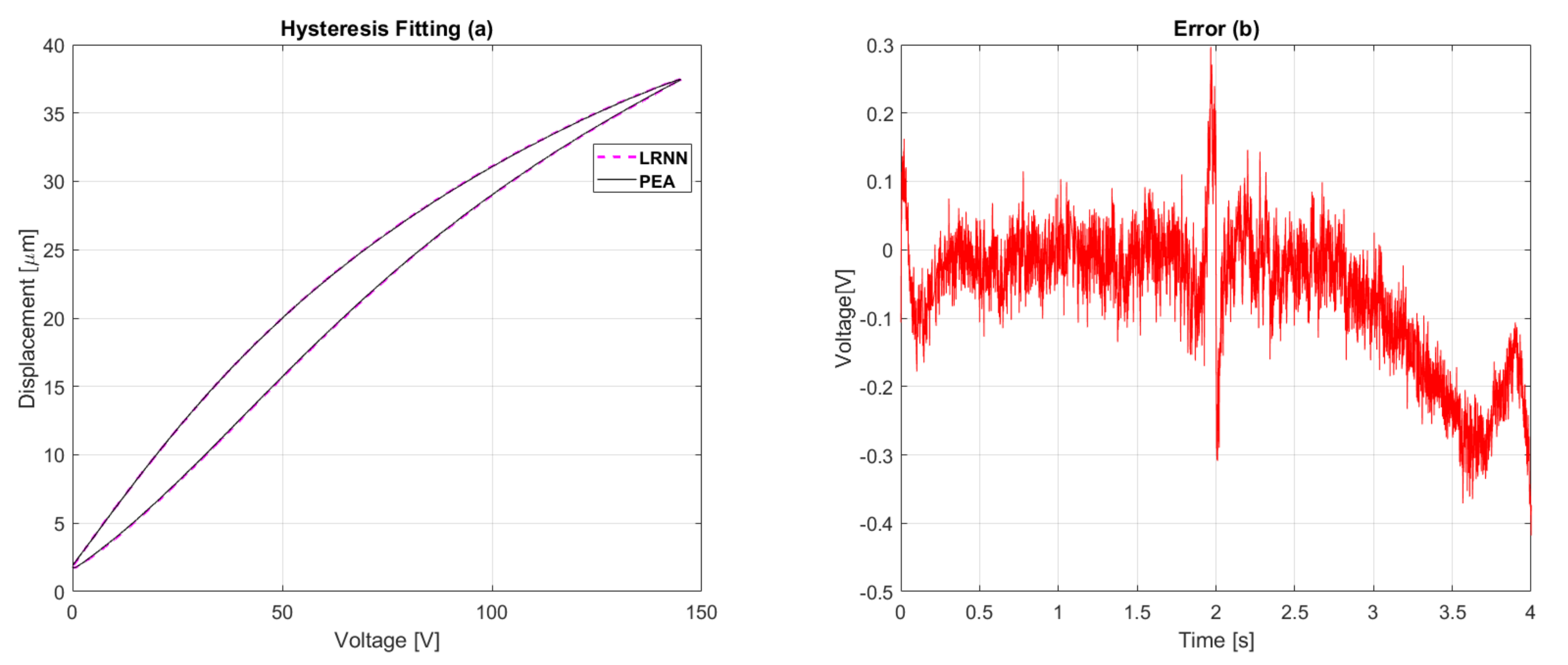
3.1. LRRN Training Results

The training of the ANN was undertaken with data recorded from the triangle input signal described in Section 2.1, which has an amplitude of 145 V and 4 s of a period. As data for training, as a compensator, the model had to be inversed, which means that the input to the LRNN was the displacement, whereas the voltage represents the output. This information not only mainly contemplates the hysteresis but also a linear compensation. A record of 40 s of data was handled and divided in 70/15/15 proportions for training, evaluation, and testing; further details are specified in

Table 3. ANN specifications.

	Values
Data points	40.000
Training/ Validation/ Test Sets	70/15/15
Iterations	5300
Performance Metric	MSE
Training Algorithm	Bayesian regularization
Training time [hs]	6

. In regards to the hardware used for iteration, a cutting-edge Dell Precision 3640 was employed and configured with parallel calculation activated in 7 cores.

The results revealed an acceptable mapping contrasted with the real data of the PEA as it is shown in Figure 6. During the first rise between 0 and 2 s, the error had a sudden fluctuation up to 0.5 s and a following variation with noise around the zero voltage up to less than 2 s. At this time value, the change of slope was expected to be sharp although the correction was performed in less than 0.05 s with 0.3 V of error. During the rise, before 2.7 s, the signal showed a leveled average again around 0 V. However, after 2.5 s the error began to plunge with intensity up to 3.5 s with noise until −0.3 V. Later, a sudden reply soared up to −0.1 V with a following fluctuation and an expected shifting that is mirrored at 0 s again due to the slope change.

Despite the fact that the error tends to fluctuate, the response is acceptable. An RMSE of 0.11 V was obtained, which is tolerable for a signal amplitude of 145 V. In addition, even if the achieved output has noise, it is also a replication of the sensor noise which was expected, as well. The inclusion of a control is able to reduce these unexpected features, can manage to diminish the error, and increase the accuracy.

3.2. Tracking Control Results

The control structures presented were embedded in the dSpace hardware, where the first one was the PID and the second one was the ST-ANN. The data acquired was produced within the two mentioned references for each controller which outcome in two different comparisons. The performance metric for the controllers tuning in real time was the IAE which had to be reduced so as to obtain outstanding results. Moreover, to secure the equipment, each structure had security blocks, like saturations (0–150 VCC of input voltage) and antiwind-up, for the integral action terms.

Regarding the gains obtained, $K_p$, $K_i$, and $K_d$ were settled to 1000, 10, and ${10}^{-4}$, respectively, for the PID. The advance architecture of ST-ANN achieves its best performance with $\lambda$, $K_1$, and $K_2$ at, respectively, values of 20, 1.4, and 118. These parameters were obtained in real-time by the reduction performance of IAE by taking into account the conditions provided by the stability proof.

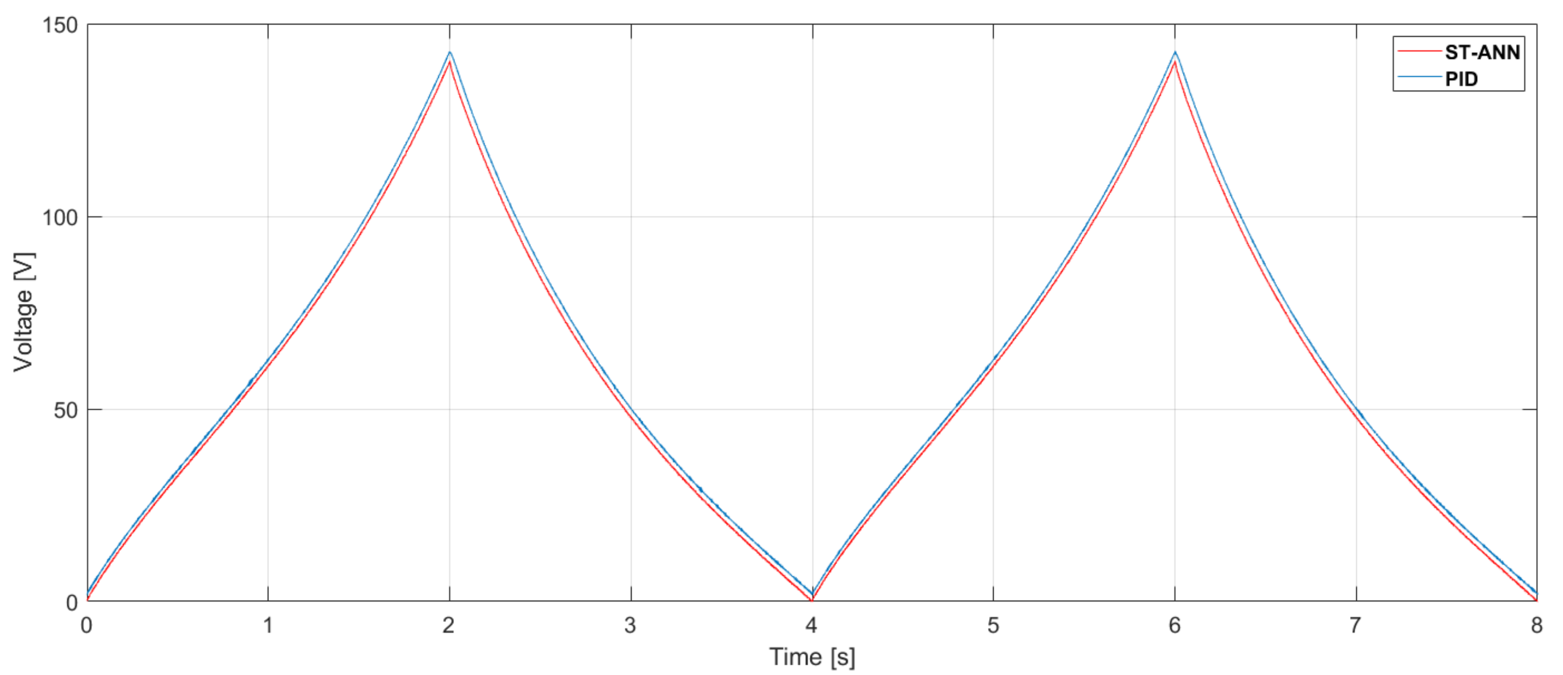
3.3. Triangle Reference Comparisons

The first comparison was allowed with the main trajectory that was used for the ANN training and also because it was a complex reference to be followed. Figure 7 is the error along 8 s (2 cycles) of a period and 145 V of amplitude. Despite the fact that the PID generates an error between 0.05 and 0.15 μm, this value decreases the performance in a guidance requirement. From the beginning, the first rise between 0 and 2 s, the PID had reduced its accuracy due to a gap from zero error, which slightly increases its value until the first slope change into negative at 2 s. Nonetheless, the ST-ANN shows a stabilized error signal with a mean near the zero and with a variation less than 0.05 μm, mostly through the first 2 s of analysis.

The following point of interest is at 2 s, where the trajectory changes promptly its slope. The shifting behavior of the PID at the upper converging point produces a sudden error correction which lasts a few fractions of a second. The error reverses its sign and value from 0.1 to near −0.15 μm, which implies a change of 0.25 μm. In spite of the perceptible slope change that the PID control tried to compensate as fast as it could, the ST-ANN acts with a subtle demeanor, as can be seen in the zoom window, where a slight overrun is performed and corrected promptly. This difference showed that the PID overshoots 2.3 more than the ST-ANN.

Between 2 and 4 s, the descending occurs, and the PID has mirrored manner, as previously during the rise but with less variation. However, the ST-ANN is still in a same performance as previously, where the level is around the zero value and with slight error increments between 3 and 4 s. At the lower converging point (at 4 s), the slope changed back to positive where the PID alternates with lower amplitude in the error switch from −0.05 to near 0.07 μm; the ST-ANN displays imperceptible changes during this moment as can be seen in the following zoom window. Thereafter, the situation is repeated due to the second triangle cycle achieved each 4 s.

During the described error compensation of both architectures, a control signal was generated for the PEA and recorded to be displayed in Figure 8. Any saturation or sudden changes were exposed which could damage the PEA driver or even reach the instability. Although the complex control framework incorporates a discontinuous term, the generated control signal is acceptable since chattering was unnoticed.

3.4. Sine Reference Comparisons

The triangular trajectories showed a suitable tracking performance, and it was expected to increment on the effectiveness for a soft reference with the same features (like amplitude and period) as a sine wave. However, in Figure 9, it can be seen that the PID still has difficulties to follow a soft signal, although it could respond with a mild correction compared to previous results. On the other hand, the ST-ANN could manage the error even related to the sharp previous tested signal as the magnitude was around the same values. As in the similarity in amplitude (between −0.15 and 0.1 μm between 1 and 3 s), the shifting of the slope operates in a similar mien.

Since the current reference signal was soft, it was predicted that the control signal was going to behave the same, in this case, provided that a suitable control was designed. The comparison in Figure 10 shows a smooth manner in both architectures with any aggravations that could complicate the life-span of the PEA.

3.5. Performance Metrics Comparison

In this research, the prime objective was to pursuit an error reduction in the mentioned trajectories so as to increase the accuracy. Consequently, the IAE was reduced by tuning of the corresponding gains; thus, the metrics in terms of the error were calculated along a period of the reference signals already used.

Table 4. Comparison of the different metrics.

Reference	IAE			RMSE [μm]			RRMSE [%]
	ST	PID	Difference	ST-ANN	PID	Difference	ST	PID	Difference
Triangle	0.0653	0.28	4.2×	0.0203	0.0756	3.7×	0.45	1.69	3.75×
Sine wave	0.0625	0.28	4.4×	0.0195	0.0795	4×	0.44	1.80	4.09×

shows the results of the IAE, RMSE, and RRMSE contrasted in both controllers and signals.

The IAE revealed an expected improvement for the ST-ANN, where the PID showed 0.28 in both references but the ST-ANN increased the precision with the sine wave by twice (from 0.065 in the triangle up to 0.0625 with the sine wave). This dissimilarity is reflected in both cases where the ST-ANN enhanced 4.2 and 4.4 times in difference.

Regarding the RMSE, the reflection is similar with the same magnitude of variation. The ST-ANN yielded an RMSE of 0.0203 μm with a triangle trajectory, whereas the PID downgraded the performance to 0.0756 μm, which implies a difference of 3.7 times. The sine wave was expected to show a similar and even greater disparity, which is expressed 4 times higher for the PID.

Finally, the RRMSE endures the previous trend where the ST-ANN overcame the comparisons. The situation was likewise with the triangular reference: the PID showed a value of 1.69%, whereas the ST-ANN diminished up to 0.45%, resulting in 3.75 times of difference. Again, the circumstance is similar in the sine wave trajectory where the magnitudes are alike and the difference is higher as expected.

4. Conclusions

In the current research, it was proven that PEA actuators can gather high accuracy in terms of micro-displacement in a way required for special applications, like that reviewed in Section 1. Hysteresis is one of the key obstacles, so a suitable and advanced control should be designed to accomplish the target of reducing the nonlinearity.

In this study, a commercial PEA from Thorlabs with its peripheral hardware was used to test each control structure designed in a dSpace board. At first, it was shown that the hysteresis provided by the manufacturer can reach up to 15%. A triangular reference of 145 VCC of amplitude with a period of 4 s was used as the main signal, although a sine wave with the same features was tested for robustness check. It was found that HOSMC controllers are a satisfactory option to try since the chattering is fairly reduced compared to first order SMC and also due to their robustness. An ANN was used to avoid the issues that the model-based SMC represents; thus, an LRNN trained with Bayesian regularization was developed with real data from the PEA.

A Lyapunov stability proof was presented to reveal the theoretical performance of the ST-ANN. It was uncovered that the controller supplies a stable response provided that the STA accomplishes with conditions based on its gains. The following steps were the experiments based on the implementation of the control architectures; the gains of each framework were tuned based on $minIAE$. The stability was also check in the experiments since unstable responses were unseen. Regarding the complex reference that the triangle represented, the ST-ANN displayed a remarkable performance in comparison to the PID since the latter had variations specially in the slope changes, whereas the advance structure displayed a slight noisy fluctuation (which can be associated to the sensor) around the zero value. The error generated in the sine wave as a reference exhibited similarities with the ST-ANN, whereas the PID could not reduce the error, even if the signal was soft. In terms of the control signals, both controllers showed acceptable behaviors even in the triangle as in the sine wave where no saturations nor severe changes were appreciated. In general terms, the two controllers revealed soft and adequate signals.

At last, a comparison of metrics was performed where it was shown the advantage of the ST-ANN numerically. Regarding the IAE, both controllers had almost the same difference, but the ST-ANN exposed a higher performance, which was between 4.2 and 4.4 times superior to the PID. The other metric compared was the RMSE, which resembled a greater discrepancy in the triangle reference; the ST-ANN was 3.7 times higher, and, in the softer signal, it was increased to 4. Finally, the RRMSE act the same since the magnitudes were similar as with the RMSE.

Future research aims include various options so as to improve the performance of ST-ANN. A complex ANN can be used since a shallow type was designed; thus, a deep learning approach can be considered so as to be implemented in real time (taking into account that the computational requirement for training can be higher). Regarding the STA used, the gains were tuned based on parameter minimization and stabilization condition, but an adaptive algorithm can be also implemented, like fuzzy or neural approach.

References

1. Arnold, S.; Pertsch, P.; Spanner, K. Piezoelectric Positioning. In Piezoelectricity: Evolution and Future of a Technology; Springer: Berlin/Heidelberg, Germany, 2008; pp. 279–297. [Google Scholar] [CrossRef]
2. Liseli, J.B.; Agnus, J.; Lutz, P.; Rakotondrabe, M. An Overview of Piezoelectric Self-Sensing Actuation for Nanopositioning Applications: Electrical Circuits, Displacement, and Force Estimation. IEEE Trans. Instrum. Meas. 2020, 69, 2–14. [Google Scholar] [CrossRef] [Green Version]
3. Zhang, P. Sensors and actuators. In Advanced Industrial Control Technology; Chapter 3; Zhang, P., Ed.; Elsevier: Amsterdam, The Netherlands, 2010; pp. 73–116. [Google Scholar] [CrossRef]
4. Takashi, O.; Norikazu, O. Power-Efficient Driver Circuit for Piezo Electric Actuator with Passive Charge Recovery. Energies 2020, 13, 2866. [Google Scholar] [CrossRef]
5. Arena, M.; Viscardi, M. SISO Piezo Based Circuit Development for Active Structural Vibration Control. Fluids 2020, 5, 183. [Google Scholar] [CrossRef]
6. Ryndzionek, R.; Sienkiewicz, L.; Michna, M.; Kutt, F. Design and Experiments of a Piezoelectric Motor Using Three Rotating Mode Actuators. Sensors 2019, 19, 5184. [Google Scholar] [CrossRef] [PubMed] [Green Version]
7. Karumuri, S.; Hamza, M.; Puli, A.; Sravani, G. Design and optimization of MEMS based piezoelectric actuator for drug delivery systems. Microsyst. Technol. 2019, 26. [Google Scholar] [CrossRef]
8. Fu, Y.; Luo, J.; Flewitt, A.; Milne, W. Smart microgrippers for bioMEMS applications. In MEMS for Biomedical Applications; Woodhead Publishing: Sawston, UK, 2012; pp. 291–336. [Google Scholar] [CrossRef]
9. Meinhold, W.; Martinez, D.E.; Oshinski, J.N.; Hu, A.P.; Ueda, J. A direct drive parallel plane piezoelectric needle positioning robot for MRI guided intraspinal injection. IEEE Trans. Biomed. Eng. 2020. [Google Scholar] [CrossRef]
10. Bani-Hani, M.; Amin Karami, M. Piezoelectric Tooth Aligner for Accelerated Orthodontic Tooth Movement. In Proceedings of the 2018 40th Annual International Conference of the IEEE Engineering in Medicine and Biology Society (EMBC), Honolulu, HI, USA, 18–21 July 2018; pp. 4265–4268. [Google Scholar] [CrossRef]
11. Liu, C.; Guo, Y. Modeling and Positioning of a PZT Precision Drive System. Sensors 2017, 17, 2577. [Google Scholar] [CrossRef] [Green Version]
12. Adriaens, H.; Koning, W.; Banning, R. Modeling piezoelectric actuators. Mechatronics IEEE/ASME Trans. 2001, 5, 331–341. [Google Scholar] [CrossRef] [Green Version]
13. Stefanski, F.; Minorowicz, B. Open loop control of piezoelectric tube transducer. Arch. Mech. Technol. Mater. 2018, 38, 23–28. [Google Scholar] [CrossRef] [Green Version]
14. Zhiliang, Y.; Yue, W.; Fang, Z.; Sun, H. Modeling and compensation of hysteresis in piezoelectric actuators. Heliyon 2020, 6. [Google Scholar] [CrossRef]
15. Nafea, M.; Mohamed, Z.; Abdullahi, A.; Ahmad, M.; Husain, A. Dynamic Hysteresis Based Modeling Of Piezoelectric Actuators. J. Teknol. 2014, 67, 9–13. [Google Scholar] [CrossRef] [Green Version]
16. Li, H.; Xu, Y.; Shao, M.; Guo, L.; An, D. Analysis for hysteresis of piezoelectric actuator based on microscopic mechanism. IOP Conf. Ser. Mater. Sci. Eng. 2018, 399. [Google Scholar] [CrossRef]
17. Helke, G.; Lubitz, K. Piezoelectric PZT Ceramics. In Piezoelectricity: Evolution and Future of a Technology; Springer: Berlin/Heidelberg, Germany, 2008; pp. 89–130. [Google Scholar] [CrossRef]
18. An, D.; Li, H.; Xu, Y.; Zhang, L. Compensation of Hysteresis on Piezoelectric Actuators Based on Tripartite PI Model. Micromachines 2018, 9, 44. [Google Scholar] [CrossRef] [PubMed] [Green Version]
19. Damjanovic, D. Hysteresis in piezoelectric and ferroelectric materials. In The Science of Hysteresis; Chapter 4; Academic Press: San Diego, CA, USA, 2006; pp. 338–452. [Google Scholar] [CrossRef] [Green Version]
20. Newcomb, C.V.; Flinn, I. Improving the linearity of piezoelectric ceramic actuators. Electron. Lett. 1982, 18, 442–444. [Google Scholar] [CrossRef]
21. Cuttino, J.F.; Miller, A.C.; Schinstock, D.E. Performance optimization of a fast tool servo for single-point diamond turning machines. IEEE/ASME Trans. Mechatronics 1999, 4, 169–179. [Google Scholar] [CrossRef]
22. Ronkanen, P.; Kallio, P.; Vilkko, M.; Koivo, H.N. Displacement Control of Piezoelectric Actuators Using Current and Voltage. IEEE/ASME Trans. Mechatronics 2011, 16, 160–166. [Google Scholar] [CrossRef]
23. Lin, C.; Yang, S. Precise positioning of piezo-actuated stages using hysteresis-observer based control. Mechatronics 2006, 16, 417–426. [Google Scholar] [CrossRef] [Green Version]
24. Choi, G.; Lim, Y.; Choi, G. Tracking position control of piezoelectric actuators for periodic reference inputs. Mechatronics 2002, 12, 669–684. [Google Scholar] [CrossRef]
25. Lin, J.; Chiang, H.; Lin, C. Tuning PID control parameters for micro-piezo-stage by using grey relational analysis. Expert Syst. Appl. 2011, 38, 13924–13932. [Google Scholar] [CrossRef]
26. Abramovitch, D.; Hoen, S.; Workman, R. Semi-automatic tuning of PID gains for Atomic Force Microscopes. Asian J. Control 2008, 11, 188–195. [Google Scholar] [CrossRef]
27. Rebai, R.; Guesmi, K.; Boualem, H. Design of an optimized fractional order fuzzy PID controller for a piezoelectric actuator. Control. Eng. Appl. Informatics 2015, 17, 41–49. [Google Scholar] [CrossRef]
28. Applebaum, E.; Ben-Asher, J. Fuzzy gain scheduling using output feedback for flutter suppression in unmanned aerial vehicles with Piezoelectric materials. In Proceedings of the IEEE Annual Meeting of the Fuzzy Information, NAFIPS ’04, Banff, AL, Canada, 27–30 June 2004; Volume 1, pp. 242–247. [Google Scholar] [CrossRef]
29. Ezzraimi, M.; Tiberkak, R.; Melbous, A.; Rechak, S. LQR and PID Algorithms for Vibration Control of Piezoelectric Composite Plates. Mechanics 2018, 24. [Google Scholar] [CrossRef] [Green Version]
30. Chi, Z. Recent Advances in the Control of Piezoelectric Actuators. Int. J. Adv. Robot. Syst. 2014, 11. [Google Scholar] [CrossRef] [Green Version]
31. Oates, W.; Smith, R. Nonlinear optimal tracking control of a piezoelectric nanopositioning stage. Proc. SPIE Int. Soc. Opt. Eng. 2006, 6166. [Google Scholar] [CrossRef] [Green Version]
32. Chen, Y.; Huang, M.; Tsai, Y. Nonlinear control design of piezoelectric actuators with micro positioning capability. Microsyst. Technol. 2019. [Google Scholar] [CrossRef]
33. Song, J.; Kiureghian, A. Generalized Bouc–Wen Model for Highly Asymmetric Hysteresis. J. Eng. Mech. ASCE 2006, 132. [Google Scholar] [CrossRef] [Green Version]
34. Minh, T.; Nguyen, L.; Chen, X. Tracking control of piezoelectric actuator using adaptive model. Robot. Biomimetics 2016, 3. [Google Scholar] [CrossRef] [Green Version]
35. Dong, R.; Tan, Y. Nonlinear Robust Control of Positioning Stage Using Piezoelectric Actuator. In Proceedings of the 2018 IEEE 8th Annual International Conference on CYBER Technology in Automation, Control, and Intelligent Systems (CYBER), Tianjin, China, 19–23 July 2018; pp. 204–207. [Google Scholar] [CrossRef]
36. Draženović, B.; Milosavljevi, C.; Veselić, B. Comprehensive Approach to Sliding Mode Design and Analysis in Linear Systems. In Advances in Sliding Mode Control: Concept, Theory and Implementation; Springer: Berlin/Heidelberg, Germany, 2013; pp. 1–19. [Google Scholar] [CrossRef]
37. Derbeli, M.; Sbita, L.; Farhat, M.; Barambones, O. PEM fuel cell green energy generation—SMC efficiency optimization. In Proceedings of the 2017 International Conference on Green Energy Conversion Systems (GECS), Hammamet, Tunisia, 23–25 March 2017; pp. 1–5. [Google Scholar] [CrossRef]
38. Velasco, J.; Barambones, O.; Calvo, I.; Zubia, J.; Saez de Ocariz, I.; Chouza, A. Sliding Mode Control with Dynamical Correction for Time-Delay Piezoelectric Actuator Systems. Materials 2019, 13, 132. [Google Scholar] [CrossRef] [Green Version]
39. Huang, P.; Shieh, P.; Lin, F.; Shieh, H. Sliding-mode control for a two-dimensional piezo-positioning stage. IET Control. Theory Appl. 2007, 1, 1104–1113. [Google Scholar] [CrossRef]
40. Shen, J.; Jywe, W.; Liu, C.; Jian, Y.; Yang, J. Sliding-mode control of a three-degrees-of-freedom nanopositioner. Asian J. Control 2008, 10, 267–276. [Google Scholar] [CrossRef]
41. Velasco, J.; Calvo, I.; Barambones, O.; Venegas, P.; Napole, C. Experimental Validation of a Sliding Mode Control for a Stewart Platform Used in Aerospace Inspection Applications. Mathematics 2020, 8, 2051. [Google Scholar] [CrossRef]
42. Chouza, A.; Barambones, O.; Calvo, I.; Velasco, J. Sliding Mode-Based Robust Control for Piezoelectric Actuators with Inverse Dynamics Estimation. Energies 2019, 12, 943. [Google Scholar] [CrossRef] [Green Version]
43. Thanh, H.; Vu, M.; Mung, X.; Nguyen, N.P.; Phuong, N. Perturbation Observer-Based Robust Control Using a Multiple Sliding Surfaces for Nonlinear Systems with Influences of Matched and Unmatched Uncertainties. Mathematics 2020, 8, 1371. [Google Scholar] [CrossRef]
44. Lin, H.; Leon, J.; Luo, W.; Marquez, A.; Liu, J.; Vazquez, S.; Franquelo, L. Integral Sliding-Mode Control-Based Direct Power Control for Three-Level NPC Converters. Energies 2020, 13, 227. [Google Scholar] [CrossRef] [Green Version]
45. Zaihidee, M.; Mekhilef, S.; Mubin, M. Robust Speed Control of PMSM Using Sliding Mode Control (SMC)—A Review. Energies 2019, 12, 1669. [Google Scholar] [CrossRef] [Green Version]
46. Chen, S.; Kuo, C. Design and implementation of double-integral sliding-mode controller for brushless direct current motor speed control. Adv. Mech. Eng. 2017, 9, 1687814017737724. [Google Scholar] [CrossRef] [Green Version]
47. Fridman, L.; Levant, A. Higher-Order Sliding Modes. In Sliding Mode Control in Engineering; Taylor and Francis Group: New York, NY, USA, 2002; Volume 11, pp. 53–101. [Google Scholar] [CrossRef]
48. Silaa, M.; Derbeli, M.; Barambones, O.; Cheknane, A. Design and Implementation of High Order Sliding Mode Control for PEMFC Power System. Energies 2020, 13, 4317. [Google Scholar] [CrossRef]
49. Derbeli, M.; Barambones, O.; Silaa, M.; Napole, C. Real-Time Implementation of a New MPPT Control Method for a DC-DC Boost Converter Used in a PEM Fuel Cell Power System. Actuators 2020, 9, 105. [Google Scholar] [CrossRef]
50. Shahid, Y.; Wei, M. Comparative Analysis of Different Model-Based Controllers Using Active Vehicle Suspension System. Algorithms 2019, 13, 10. [Google Scholar] [CrossRef] [Green Version]
51. Huo, R.; Liu, X.; Zeng, X.; Lei, Z. Integrated guidance and control based on high-order sliding mode method. In Proceedings of the 2017 36th Chinese Control Conference (CCC), Dalian, China, 26–28 July 2017; pp. 6073–6078. [Google Scholar] [CrossRef]
52. Liu, X.; Wang, W. High order sliding mode and its application on the tracking control of piezoelectric systems. Int. J. Innov. Comput. Inf. Control 2008, 4, 697–704. [Google Scholar]
53. Wang, Y.; Su, H.; Harrington, K.; Fischer, G. Sliding Mode Control of Piezoelectric Valve Regulated Pneumatic Actuator for MRI-Compatible Robotic Intervention. In Proceedings of the ASME 2010 Dynamic Systems and Control Conference, DSCC2010, Cambridge, MA, USA, 12–15 September 2010; Volume 2. [Google Scholar] [CrossRef]
54. Abidi, K.; Sabanovic, A.; Yannier, S. Experimental investigation of a SMC high precision control. In Proceedings of the 9th IEEE International Workshop on Advanced Motion Control, Istanbul, Turkey, 27–29 March 2006; pp. 721–726. [Google Scholar] [CrossRef] [Green Version]
55. Derbeli, M.; Barambones, O.; Farhat, M.; Ramos-Hernanz, J.A.; Sbita, L. Robust high order sliding mode control for performance improvement of PEM fuel cell power systems. Int. J. Hydrogen Energy 2020, 45, 29222–29234. [Google Scholar] [CrossRef]
56. Yan, Y.; Yu, Y. Quantization Behaviors in Equivalent-Control Based Sliding-Mode Control Systems. In Advances in Sliding Mode Control: Concept, Theory and Implementation; Springer: Berlin/Heidelberg, Germany, 2013; pp. 221–241. [Google Scholar] [CrossRef]
57. Napole, C.; Barambones, O.; Calvo, I.; Derbeli, M.; Silaa, M.; Velasco, J. Advances in Tracking Control for Piezoelectric Actuators Using Fuzzy Logic and Hammerstein-Wiener Compensation. Mathematics 2020, 8, 2071. [Google Scholar] [CrossRef]
58. Armin, M.; Roy, P.N.; Das, S.K. A Survey on Modelling and Compensation for Hysteresis in High Speed Nanopositioning of AFMs: Observation and Future Recommendation. Int. J. Autom. Comput. 2020, 17, 479. [Google Scholar] [CrossRef]
59. Xiong, R.; Liu, X.; Lai, Z. Modeling of Hysteresis in Piezoelectric Actuator Based on Segment Similarity. Micromachines 2015, 6, 1805–1824. [Google Scholar] [CrossRef] [Green Version]
60. Huang, L.; Hu, Y.; Zhao, Y.; X, L. Modeling and Control of IPMC Actuators Based on LSSVM-NARX Paradigm. Mathematics 2019, 7, 741. [Google Scholar] [CrossRef] [Green Version]
61. Xu, R.; Tian, D.; Wang, Z. Adaptive Tracking Control for the Piezoelectric Actuated Stage Using the Krasnosel’skii-Pokrovskii Operator. Micromachines 2020, 11, 537. [Google Scholar] [CrossRef] [PubMed]
62. Carneiro, F.; Abreu, P.; Restivo, M. Hysteresis Compensation in a Tactile Device for Arterial Pulse Reproduction. Sensors 2018, 18, 1631. [Google Scholar] [CrossRef] [Green Version]
63. Lin, J.; Chiang, M. Tracking Control of a Magnetic Shape Memory Actuator Using an Inverse Preisach Model with Modified Fuzzy Sliding Mode Control. Sensors 2016, 16, 1368. [Google Scholar] [CrossRef] [Green Version]
64. Vaiana, N.; Sessa, S.; Marmo, F.; Rosati, L. A class of uniaxial phenomenological models for simulating hysteretic phenomena in rate-independent mechanical systems and materials. Nonlinear Dyn. 2018, 93. [Google Scholar] [CrossRef]
65. Vaiana, N.; Sessa, S.; Rosati, L. A generalized class of uniaxial rate-independent models for simulating asymmetric mechanical hysteresis phenomena. Mech. Syst. Signal Process. 2021, 146, 106984. [Google Scholar] [CrossRef]
66. Napole, C.; Barambones, O.; Calvo, I.; Velasco, J. Feedforward Compensation Analysis of Piezoelectric Actuators Using Artificial Neural Networks with Conventional PID Controller and Single-Neuron PID Based on Hebb Learning Rules. Energies 2020, 13, 3929. [Google Scholar] [CrossRef]
67. Napole, C.; Barambones, O.; Derbeli, M.; Silaa, M.; Calvo, I.; Velasco, J. Tracking Control for Piezoelectric Actuators with Advanced Feed-forward Compensation Combined with PI Control. In Proceedings of the 1st International Electronic Conference on Actuator Technology, Online, 23–27 November 2020. [Google Scholar] [CrossRef]
68. Valenzuela, F.; Reymundo, R.; Martínez, F.; Onofre, A.; Castañeda, C.E. Super-Twisting Algorithm Applied to Velocity Control of DC Motor without Mechanical Sensors Dependence. Energies 2020, 13, 6041. [Google Scholar] [CrossRef]
69. Khan, R.; Khan, L.; Ullah, S.; Sami, I.; Ro, J. Backstepping Based Super-Twisting Sliding Mode MPPT Control with Differential Flatness Oriented Observer Design for Photovoltaic System. Electronics 2020, 9, 1543. [Google Scholar] [CrossRef]
70. Gao, P.; Zhang, G.; Lv, X. Model-Free Hybrid Control with Intelligent Proportional Integral and Super-Twisting Sliding Mode Control of PMSM Drives. Electronics 2020, 9, 1427. [Google Scholar] [CrossRef]
71. Gan, J.; Zhang, X.; Wu, H. A generalized Prandtl-Ishlinskii model for characterizing the rate-independent and rate-dependent hysteresis of piezoelectric actuators. Rev. Sci. Instrum. 2016, 87, 035002. [Google Scholar] [CrossRef]
72. Li, W.; Nie, L.; Liu, Y.; Zhou, M. Rate Dependent Krasnoselskii-Pokrovskii Modeling and Inverse Compensation Control of Piezoceramic Actuated Stages. Sensors 2020, 20, 5062. [Google Scholar] [CrossRef]
73. Qin, Y.; Duan, H. Single-Neuron Adaptive Hysteresis Compensation of Piezoelectric Actuator Based on Hebb Learning Rules. Micromachines 2020, 11, 84. [Google Scholar] [CrossRef] [Green Version]
74. Soleimani Amiri, M.; Ramli, R.; Ibrahim, M.; Wahab, D.; Aliman, N. Adaptive Particle Swarm Optimization of PID Gain Tuning for Lower-Limb Human Exoskeleton in Virtual Environment. Mathematics 2020, 8, 2040. [Google Scholar] [CrossRef]
75. Zhao, Y.; Huang, X.; Liu, Y.; Wang, G.; Hong, K. Design and Control of a Piezoelectric-Driven Microgripper Perceiving Displacement and Gripping Force. Micromachines 2020, 11, 121. [Google Scholar] [CrossRef] [Green Version]
76. Cappa, P.; Rita, G.; McConnell, K.G.; Zachary, L. Using Strain Gages to Measure Both Strain and Temperature. Exp. Mech. 1992, 32, 230–233. [Google Scholar] [CrossRef]
77. Li, H.; Zhang, Z.; Liu, Z. Application of Artificial Neural Networks for Catalysis: A Review. Catalysts 2017, 7, 306. [Google Scholar] [CrossRef]
78. Allam, Z. Achieving Neuroplasticity in Artificial Neural Networks through Smart Cities. Smart Cities 2019, 2, 118–134. [Google Scholar] [CrossRef] [Green Version]
79. Nguyen, V.S. Investigation of a Multitasking System for Automatic Ship Berthing in Marine Practice Based on an Integrated Neural Controller. Mathematics 2020, 8, 1167. [Google Scholar] [CrossRef]
80. Matrenin, P.; Manusov, V.; Khalyasmaa, A.; Antonenkov, D.; Eroshenko, S.; Butusov, D. Improving Accuracy and Generalization Performance of Small-Size Recurrent Neural Networks Applied to Short-Term Load Forecasting. Mathematics 2020, 8, 2169. [Google Scholar] [CrossRef]
81. Alyukov, A.; Rozhdestvenskiy, Y.; Alyukov, S. Active Shock Absorber Control Based on Time-Delay Neural Network. Energies 2020, 13, 1091. [Google Scholar] [CrossRef] [Green Version]
82. Liu, L.; Zhu, L.; Feng, F.; Zhang, W.; Zhang, Q.; Lin, Q.; Liu, G. A Time Delay Neural Network Based Technique for Nonlinear Microwave Device Modeling. Micromachines 2020, 11, 831. [Google Scholar] [CrossRef]
83. Ahn, H.; Park, N. Deep RNN-Based Photovoltaic Power Short-Term Forecast Using Power IoT Sensors. Energies 2021, 14, 436. [Google Scholar] [CrossRef]
84. Grech, C.; Buzio, M.; Pentella, M.; Sammut, N. Dynamic Ferromagnetic Hysteresis Modelling Using a Preisach-Recurrent Neural Network Model. Materials 2020, 13, 2561. [Google Scholar] [CrossRef]
85. Beale, M.; Hagan, M.; Demuth, H. Deploy Training of Shallow Neural Networks. In Deep Learning Toolbox; The Mathworks Inc.: Natick, MA, USA, 2020; pp. 21–22. [Google Scholar]
86. Doubravová, J.; Wiszniowski, J.; Horalek, J. Single Layer Recurrent Neural Network for detection of swarm-like earthquakes in W-Bohemia/Vogtland—The method. Comput. Geosci. 2016, 93. [Google Scholar] [CrossRef]
87. Negash, B.; Yaw, A. Artificial neural network based production forecasting for a hydrocarbon reservoir under water injection. Pet. Explor. Dev. 2020, 47, 383–392. [Google Scholar] [CrossRef]
88. Okut, H. Bayesian Regularized Neural Networks for Small n Big p Data. In Artificial Neural Networks-Models and Applications; Chapter 2; Intech: London, UK, 2016; pp. 28–48. [Google Scholar] [CrossRef] [Green Version]
89. Morfin, O.; Castaneda, C.; Valderrabano-Gonzalez, A.; Hernandez-Gonzalez, M.; Valenzuela, F. A Real-Time SOSM Super-Twisting Technique for a Compound DC Motor Velocity Controller. Energies 2017, 10, 1286. [Google Scholar] [CrossRef] [Green Version]
90. Moreno, J. Lyapunov Approach for Analysis and Design of Second Order Sliding Mode Algorithms. In Sliding Modes after the First Decade of the 21st Century; Springer: Berlin/Heidelberg, Germany, 2011; Volume 412, pp. 113–149. [Google Scholar] [CrossRef]
91. Alhato, M.; Bouallègue, S.; Rezk, H. Modeling and Performance Improvement of Direct Power Control of Doubly-Fed Induction Generator Based Wind Turbine through Second-Order Sliding Mode Control Approach. Mathematics 2020, 8, 2012. [Google Scholar] [CrossRef]
92. Moreno, J.A.; Osorio, M. Strict Lyapunov Functions for the Super-Twisting Algorithm. IEEE Trans. Autom. Control 2012, 57, 1035–1040. [Google Scholar] [CrossRef]
93. Stamov, G.; Stamova, I.; Venkov, G.; Stamov, T.; Spirova, C. Global Stability of Integral Manifolds for Reaction–Diffusion Delayed Neural Networks of Cohen–Grossberg-Type under Variable Impulsive Perturbations. Mathematics 2020, 8, 1082. [Google Scholar] [CrossRef]
94. Popa, C.; Kaslik, E. Finite-Time Mittag–Leffler Synchronization of Neutral-Type Fractional-Order Neural Networks with Leakage Delay and Time-Varying Delays. Mathematics 2020, 8, 1146. [Google Scholar] [CrossRef]
95. Ramm, A. Stability of Solutions to Some Evolution Problems. Mathematics 2010, 1, 46. [Google Scholar] [CrossRef] [Green Version]
Figure 1. Piezoelectric material polarization with an electric field where: (a) is in a neutral state, (b) is with an applied field, and (c) is after the electric field action.
Mathematics 09 00244 g001
Figure 2. Hardware and software integration architecture.
Mathematics 09 00244 g002
Figure 3. PK4FYC2 hysteresis graph between 0–145 VCC.
Mathematics 09 00244 g003
Figure 4. Control architectures used during the experiments. (a) ST -artificial neural networks (ANN); (b) feedback with proportional-integral-derivative (PID).
Mathematics 09 00244 g004
Figure 5. Recurrent artificial neural network (ANN) architecture.
Mathematics 09 00244 g005
Figure 6. Performance of the Layer Recurrent Neural Network (LRNN), where: (a) hysteresis fitting; (b) error approximation.
Mathematics 09 00244 g006
Figure 7. Error comparison between the ST-ANN and the PID structures.
Mathematics 09 00244 g007
Figure 8. Control signals comparison of the ST-ANN and the PID.
Mathematics 09 00244 g008
Figure 9. Error comparison between the ST-ANN and the PID structures for a sine wave tracking reference.
Mathematics 09 00244 g009
Figure 10. Control signal comparison between the ST-ANN and the PID structures for a sine wave tracking reference.
Mathematics 09 00244 g010