A Study of ψ-Hilfer Fractional Boundary Value Problem via Nonlinear Integral Conditions Describing Navier Model

Abstract

This paper investigates existence, uniqueness, and Ulam’s stability results for a nonlinear implicit $\psi$-Hilfer $\mathbb{FBVP}$ describing Navier model with $\mathbb{NIBC}$s. By Banach’s fixed point theorem, the unique property is established. Meanwhile, existence results are proved by using the fixed point theory of Leray-Schauder’s and Krasnoselskii’s types. In addition, Ulam’s stability results are analyzed. Furthermore, several instances are provided to demonstrate the efficacy of the main results.

1. Introduction

Hundreds of years ago, fractional calculus began and has been widely interested by researchers in branches of applied mathematics, science, engineering, and so on (see References [1,2,3]). It is also known as the non-integer order (fractional-order) of differential and integral operators. Various definitions of novel fractional integral and derivative operators are currently prominent tools in numerous publications. Normally, the real-world problems were simulated using differential equations and solved the difficulties using powerful techniques (see References [4,5]). The fractional calculus has been used to examine differential equations with non-integer order (fractional differential equations ($\mathbb{FDE}$s)). $\mathbb{FDE}$s via initial/boundary conditions have also been used to solve the problems since fractional-order has more additional degrees of freedom than integer-order, allowing for more precise and realistic solutions. Researchers have considered a variety of mathematical approaches in relation to $\mathbb{FDE}$s in a large number of papers (see References [6,7,8,9,10,11,12,13,14,15,16,17,18,19]).

Elastic beams are an essential element required in structural problems, including aircraft, ships, bridges, buildings, and so on (see References [20,21,22,23,24,25,26,27,28,29,30,31,32,33,34,35,36]). In the sense of mathematical analysis, the deformation of the beam can be analyzed using the fourth-order boundary value problem ($\mathbb{BVP}$) describing the Navier model [37]:

$$\left\{\begin{array}{c}{\displaystyle u^{\left(4\right)}\left(\tau \right)=g(\tau ,u\left(\tau \right),u^{\prime \prime }\left(\tau \right)),\tau \in (0,1),}\hfill \\ {\displaystyle u\left(0\right)=u\left(1\right)=u^{\prime \prime }\left(0\right)=u^{\prime \prime }\left(1\right)=0,}\hfill \end{array}\right.$$

(1)

where $g\in \mathcal{C}([0,1]\times {\mathbb{R}}^2,\mathbb{R})$. Problem (1) has attracted the attention of many researchers due to its dominance in the field of mechanics. It simulates the bending equilibrium of a beam supported at both ends by an elastic basis. We will go through some important works on the subject shortly below. For instance, in 1986, Aftabizadeh [38] converted (1) into a second-order integro-differential equation with f is bounded on $[0,1]\times {\mathbb{R}}^2$. The existence results were analyzed by Schauder’s fixed point theorem. In 1997, Ma et al. [39] examined the existence of a solution for (1) by applying the upper and lower solutions method. After that, in 2004, Bai et al. [40] developed upper and lower solutions of (1). Dang et al. [41] examined the problem (1) by reducing it to an operator equation and using some simply confirmed conditions. In recent years, many literature examples pay attention to $\mathbb{BVP}$s under many kinds of fractional derivatives; for instance, in 2020, Bachar and Eltayeb [42] studied the Navier $\mathbb{BVP}$ under Riemann-Liouville ($\mathbb{RL}$) fractional derivative type:

$$\left\{\begin{array}{c}{\displaystyle {}^{\mathbb{RL}}{\mathfrak{D}}_{0^{+}}^{\alpha }\left({}^{\mathbb{RL}}{\mathfrak{D}}_{0^{+}}^{\beta }u\right)\left(\tau \right)=g(\tau ,u\left(\tau \right),{}^{\mathbb{RL}}{\mathfrak{D}}_{0^{+}}^{\beta }u\left(\tau \right)),\tau \in (0,1),}\hfill \\ {\displaystyle u\left(0\right)={}^{\mathbb{RL}}{\mathfrak{D}}_{0^{+}}^{\beta }u\left(0\right)=u\left(1\right)={}^{\mathbb{RL}}{\mathfrak{D}}_{0^{+}}^{\beta }u\left(1\right)=0,}\hfill \end{array}\right.$$

(2)

where ${}^{\mathbb{RL}}{\mathfrak{D}}_{0^{+}}^q$ denotes the $\mathbb{RL}$-fractional derivative of order $q=\{\alpha ,\beta \}\in (1,2]$ and $g\in \mathcal{C}([0,1],{\mathbb{R}}^2)$. The Green properties and helpful inequality technique are used to establish the uniqueness result of positive solutions for (2). $\mathbb{FDE}$s have been discussed in depth by several researchers. Clearly, the existence, uniqueness, and stability analysis of solutions are some important properties of $\mathbb{FDE}$s. Because the exact solution to differential equations or $\mathbb{FDE}$s is quite difficult, several researchers have attempted to identify the best technique to access the existence results. To establish the existence and stability of solutions for $\mathbb{FDE}$s, several analytical techniques, including fixed-point theory, have been investigated. Ulam’s stability is one of the most useful strategies which guarantee that there exists a close exact solution. Ulam’s stability has four types, such as Ulam–Hyers ($\mathbb{UH}$), generalized Ulam–Hyers ($\mathbb{GUH}$), Ulam–Hyers–Rassias ($\mathbb{UHR}$), and generalized Ulam–Hyers–Rassias ($\mathbb{GUHR}$) stabilities; see References [43,44,45,46,47,48,49,50,51,52,53,54] and references cited therein. However, to the authors’ knowledge, a few papers involving the Navier model in sense of $\psi$-Hilfer fractional operators have been concerned.

As a result of the preceding debates, we discuss a new class of nonlinear implicit $\psi$-Hilfer $\mathbb{FBVP}$ describing Navier model with nonlinear integral boundary conditions ($\mathbb{NIBC}$s):

$$\left\{\begin{array}{c}{\displaystyle {}^H{\mathfrak{D}}_{a^{+}}^{\alpha ,\rho ;\psi }\left({}^H{\mathfrak{D}}_{a^{+}}^{\beta ,\rho ;\psi }u\right)\left(\tau \right)=f(\tau ,u\left(\tau \right),\left(\mathcal{K}u\right)\left(\tau \right),\left(\mathcal{W}u\right)\left(\tau \right)),\tau \in (a,b),}\hfill \\ {\displaystyle u\left(a\right)=0,{}^H{\mathfrak{D}}_{a^{+}}^{\beta ,\rho ;\psi }u\left(a\right)=0,}\hfill \\ {\displaystyle \sum _{i=1}^m{\xi }_{i}u\left({\eta }_i\right)={\mathcal{I}}_{a^{+}}^{\phi ;\psi }\mathcal{G}(\sigma ,u\left(\sigma \right)),\sum _{j=1}^n{\mu }_j{}^H{\mathfrak{D}}_{a^{+}}^{{\varphi }_j,\rho ;\psi }u\left({\lambda }_j\right)={\mathcal{I}}_{a^{+}}^{\nu ;\psi }\mathcal{H}(\zeta ,u\left(\zeta \right)),}\hfill \end{array}\right.$$

(3)

where ${}^H{\mathfrak{D}}_{a^{+}}^{q,\rho ;\psi }$ denotes $\psi$-Hilfer fractional derivative of order $q=\{\alpha ,\beta ,{\varphi }_j\}$, $\alpha$, $\beta$, ${\varphi }_j\in (1,2]$, $j=1,2,\dots ,n$, $\rho \in [0,1]$, ${\mathcal{I}}_{a^{+}}^{v;\psi }$ denotes $\psi$-$\mathbb{RL}$-fractional integral of order $v=\{\phi ,\nu \}>0$, $f\in \mathcal{C}(\mathcal{J}\times {\mathbb{R}}^3,\mathbb{R})$, $\mathcal{G}$, $\mathcal{H}\in \mathcal{C}(\mathcal{J},\mathbb{R})$, $\mathcal{J}:=[a,b]$, $b>a>0$, $\sigma$, $\zeta$, ${\xi }_i$, ${\mu }_j\in \mathbb{R}$, $\sigma$, $\zeta$, ${\eta }_i$, ${\lambda }_j\in (a,b)$, $i=1,2,\dots ,m$, $j=1,2,\dots ,n$, and

$$\begin{array}{ccc}\hfill \left(\mathcal{K}u\right)\left(\tau \right)& =& \frac{1}{\mathrm{\Gamma }\left(\theta \right)}{\int }_a^{\tau }{\left(\psi \left(\tau \right)-\psi \left(s\right)\right)}^{\theta -1}{\psi }^{\prime }\left(s\right)k(\tau ,s)u\left(s\right)ds,\tau \in \mathcal{J},\hfill \end{array}$$

(4)

$$\begin{array}{ccc}\hfill \left(\mathcal{W}u\right)\left(\tau \right)& =& \frac{1}{\mathrm{\Gamma }\left(\delta \right)}{\int }_a^{\tau }{\left(\psi \left(\tau \right)-\psi \left(s\right)\right)}^{\delta -1}{\psi }^{\prime }\left(s\right)w(\tau ,s)u\left(s\right)ds,\tau \in \mathcal{J},\hfill \end{array}$$

(5)

where k, $w\in \mathcal{C}({\mathcal{J}}^2,[a,\infty ))$. The existence and uniqueness property is proved by using Banach’s fixed point theorem (Lemma 5), and the existence properties are derived by applying Leray-Schauder’s nonlinear alternative (Lemma 8) and Krasnoselskii’s fixed point theorems (Lemma 9) for the $\psi$-Hilfer $\mathbb{FBVP}$ describing Navier model with $\mathbb{NIBC}$s (3). We employ $\mathbb{UH}$, $\mathbb{GUH}$, $\mathbb{UHR}$, and $\mathbb{GUHR}$ stables to investigate the stability of (3). Finally, we give some numerical examples of various functions that were explored in order to confirm the theoretical results. In addition, we give our findings on a broad platform that covers a wide area of specific situations for different values $\rho$ and $\psi$. For example, $\psi$-Riemann-Liouville problem if $\rho =0$, $\psi$-Caputo problem if $\rho =1$, Riemann-Liouville $\mathbb{BVP}$ if $\rho =0$, $\psi \left(\tau \right)=\tau$, Caputo problem if $\rho =1$, $\psi \left(\tau \right)=\tau$, Hilfer problem if $\psi \left(\tau \right)=\tau$, Katugampola problem if $\psi \left(\tau \right)={\tau }^q$, Hilfer-Hadamard problem if $\psi \left(\tau \right)=log\left(\tau \right)$, and so on. The received results are improved: if $\alpha =2$, $\beta =2$, $\rho =1$, and $\psi \left(t\right)=t$, then we obtained Reference [41]; if $\rho =1$ and $\psi \left(t\right)=t$, then we obtained Reference [42].

This paper is structured the continuing parts of the paper as follows: In Section 2, we provide an essential system of symbols, definitions, and lemmas of $\psi$-Hilfer fractional calculus. Next, we state a lemma which is used in proving the main results. In Section 3, fixed point theorems are used to obtain the existence results of the proposed problem. By helping with the nonlinear analysis method, in Section 4, we analyze various of Ulam’s stability for the problem. Examples illustrate to confirm the effectiveness of the acquired theoretical results in Section 5. Finally, the conclusion and discussion of this paper are presented in Section 6.

2. Preliminaries

We provide the basic concepts of $\psi$-Hilfer fractional calculus, as well as important crucial results that will be engaged in this paper. Assume that $\mathcal{E}=\mathcal{C}(\mathcal{J},\mathbb{R})$ is the Banach space of continuous functions on $\mathcal{J}$ with $\parallel u\parallel ={sup}_{\tau \in \mathcal{J}}\left\{\right|u\left(\tau \right)\left|\right\}$. Assume that ${\mathcal{AC}}^n(\mathcal{J},\mathbb{R})$ is the space of n-times absolutely continuous functions with ${\mathcal{AC}}^n(\mathcal{J},\mathbb{R})=\{u:\mathcal{J}\to \mathbb{R};u^{(n-1)}\in \mathcal{AC}(\mathcal{J},\mathbb{R})\}$.

Definition 1.

(Reference [3]). Assume that $\psi \left(\tau \right)\in {\mathcal{C}}^1(\mathcal{J},\mathbb{R})$ is an increasing function with ${\psi }^{\prime }\left(\tau \right)\ne 0$ for each $\tau \in \mathcal{J}$. The ψ-$\mathbb{RL}$-fractional integral of order α of f depending on ψ on $\mathcal{J}$ is defined by

$${\mathcal{I}}_{a^{+}}^{\alpha ;\psi }f\left(\tau \right)=\frac{1}{\mathrm{\Gamma }\left(\alpha \right)}{\int }_a^{\tau }{\left(\psi \left(\tau \right)-\psi \left(s\right)\right)}^{\alpha -1}{\psi }^{\prime }\left(s\right)f\left(s\right)ds,\tau >a>0,\alpha >0,$$

where $\mathrm{\Gamma }(·)$ is the Gamma function.

Definition 2.

(Reference [3]). Assume that $\psi \left(\tau \right)$ is defined as in Definition with ${\psi }^{\prime }\left(\tau \right)\ne 0$. The ψ-$\mathbb{RL}$-fractional derivative of f depending on ψ is defined as ${\mathfrak{D}}_{a^{+}}^{\alpha ;\psi }f\left(\tau \right)={\left(\frac{1}{{\psi }^{\prime }\left(\tau \right)}\frac{d}{d\tau }\right)}^n{\mathcal{I}}_{a^{+}}^{n-\alpha ;\psi }f\left(\tau \right)$ or

$${\mathfrak{D}}_{a^{+}}^{\alpha ;\psi }f\left(\tau \right)=\frac{1}{\mathrm{\Gamma }(n-\alpha )}{\left(\frac{1}{{\psi }^{\prime }\left(\tau \right)}\frac{d}{d\tau }\right)}^n{\int }_a^{\tau }{\left(\psi \left(\tau \right)-\psi \left(s\right)\right)}^{n-\alpha -1}{\psi }^{\prime }\left(s\right)f\left(s\right)ds,\alpha >0,$$

where $n=\left[\alpha \right]+1$, and $\left[\alpha \right]$ is an integer part of $Re\left(\alpha \right)$.

Definition 3.

(Reference [55]). Assume that $\gamma =\alpha +\rho (n-\alpha )$, $\alpha \in (n-1,n)$ with $n\in \mathbb{N}$, $f\in {\mathcal{C}}^n(\mathcal{J},\mathbb{R})$ and $\psi \left(\tau \right)\in {\mathcal{C}}^1(\mathcal{J},\mathbb{R})$ is increasing with ${\psi }^{\prime }\left(\tau \right)\ne 0$ for each $\tau \in \mathcal{J}$. Then, the ψ-Hilfer fractional derivative of type $\rho \in [0,1]$ of f depending on ψ is defined as

$${}^H{\mathfrak{D}}_{a^{+}}^{\alpha ,\rho ;\psi }f\left(\tau \right)={\mathcal{I}}_{a^{+}}^{\rho (n-\alpha );\psi }{\left(\frac{1}{{\psi }^{\prime }\left(\tau \right)}\frac{d}{d\tau }\right)}^n{\mathcal{I}}_{a^{+}}^{(1-\rho )(n-\alpha );\psi }f\left(\tau \right)={\mathcal{I}}_{a^{+}}^{\gamma -\alpha ;\psi }{}^{}{\mathfrak{D}}_{a^{+}}^{\gamma ;\psi }f\left(\tau \right),$$

where ${}^{}{\mathfrak{D}}_{a^{+}}^{\gamma ;\psi }f\left(\tau \right)={}^{}{\mathfrak{D}}_{a^{+}}^{n;\psi }{\mathcal{I}}_{a^{+}}^{(1-\rho )(n-\alpha );\psi }f\left(\tau \right)$.

Lemma 1.

(Reference [3]). Assume that $\alpha ,\beta >0$. Then, ${\mathcal{I}}_{a^{+}}^{\alpha ;\psi }{\mathcal{I}}_{a^{+}}^{\beta ;\psi }f\left(\tau \right)={\mathcal{I}}_{a^{+}}^{\alpha +\beta ;\psi }f\left(\tau \right)$, $\tau >a$.

Proposition 1.

(References [3,55]). Assume that $\tau >a$ and ${\mathcal{G}}^{\upsilon }\left(\tau \right)={\left(\psi \left(\tau \right)-\psi \left(a\right)\right)}^{\upsilon }$. Then, for $\upsilon >0$, $\alpha \ge 0$, we have

(i) 

${\mathcal{I}}_{a^{+}}^{\alpha ;\psi }{\mathcal{G}}^{\upsilon -1}\left(\tau \right)=\frac{\mathrm{\Gamma }\left(\upsilon \right)}{\mathrm{\Gamma }(\upsilon +\alpha )}{\mathcal{G}}^{\upsilon +\alpha -1}\left(\tau \right)$;

(ii) 

${\mathfrak{D}}_{a^{+}}^{\alpha ,\rho ;\psi }{\mathcal{G}}^{\upsilon -1}\left(\tau \right)=\frac{\mathrm{\Gamma }\left(\upsilon \right)}{\mathrm{\Gamma }(\upsilon -\alpha )}{\mathcal{G}}^{\upsilon -\alpha -1}\left(\tau \right)$;

(iii) 

${{}^H\mathfrak{D}}_{a^{+}}^{\alpha ,\rho ;\psi }{\mathcal{G}}^{\upsilon -1}\left(\tau \right)=\frac{\mathrm{\Gamma }\left(\upsilon \right)}{\mathrm{\Gamma }(\upsilon -\alpha )}{\mathcal{G}}^{\upsilon -\alpha -1}\left(\tau \right),\upsilon >\gamma =\alpha +\rho (n-\alpha )$.

Lemma 2.

(Reference [55]) Assume that $f\in {\mathcal{C}}^n(\mathcal{J},\mathbb{R})$, $\alpha \in (n-1,n)$, $\rho \in [0,1]$, $\gamma =\alpha +\rho (n-\alpha )$. Then, we obtain

$${\mathcal{I}}_{a^{+}}^{\alpha ;\psi }{}^H{\mathfrak{D}}_{a^{+}}^{\alpha ,\rho ;\psi }f\left(\tau \right)=f\left(\tau \right)-\sum _{k=1}^n\frac{{\left(\psi \left(\tau \right)-\psi \left(a\right)\right)}^{q-k}}{\mathrm{\Gamma }(q-k+1)}{f}_{\psi }^{[n-k]}{\mathcal{I}}_{a^{+}}^{(1-\rho )(n-\alpha );\psi }f\left(a\right),$$

for all $\tau \in \mathcal{J}$, where $f_{\psi }^{\left[n\right]}f\left(\tau \right):={\left(\frac{1}{{\psi }^{\prime }\left(\tau \right)}\frac{d}{dt}\right)}^{n}f\left(\tau \right)$.

Lemma 3.

(Reference [51]) Assuming that $\alpha \in (m-1,m)$, $\beta \in (n-1,n)$, n, $m\in \mathbb{N}$, $n\le m$, $\rho \in [0,1]$, and $\alpha >\beta +\rho (n-\beta )$. If $f\in {\mathcal{C}}_{1-\gamma ,\psi }(\mathcal{J},\mathbb{R})$, then ${{}^H\mathfrak{D}}_{a^{+}}^{\beta ,\rho ;\psi }{\mathcal{I}}_{a^{+}}^{\alpha ;\psi }f\left(\varsigma \right)={\mathcal{I}}_{0^{+}}^{\alpha -\beta ;\psi }f\left(\varsigma \right)$.

Lemma 4.

Let α, β, ${\varphi }_j\in (1,2]$, $(j=1,2,\dots ,n)$, $\rho \in [0,1]$, ${\gamma }_1=\alpha +\rho (2-\alpha )$, ${\gamma }_2=\beta +\rho (2-\beta )$, ω, φ, $\nu >0$. Suppose that $h\in \mathcal{E}$ and $\mathrm{\Omega }={\mathrm{\Omega }}_{11}{\mathrm{\Omega }}_{22}-{\mathrm{\Omega }}_{12}{\mathrm{\Omega }}_{21}\ne 0$. Then, $u\in {\mathcal{C}}^2(\mathcal{J},\mathbb{R})$ is a solution of

$$\left\{\begin{array}{c}{\displaystyle {}^H{\mathfrak{D}}_{a^{+}}^{\alpha ,\rho ;\psi }\left({}^H{\mathfrak{D}}_{a^{+}}^{\beta ,\rho ;\psi }u\right)\left(\tau \right)=h\left(\tau \right),\tau \in (a,b),}\hfill \\ {\displaystyle u\left(a\right)=0,{}^H{\mathfrak{D}}_{a^{+}}^{\beta ,\rho ;\psi }u\left(a\right)=0,}\hfill \\ {\displaystyle \sum _{i=1}^m{\xi }_{i}u\left({\eta }_i\right)={\mathcal{I}}_{a^{+}}^{\phi ;\psi }\mathcal{G}(\sigma ,u\left(\sigma \right)),\sum _{i=1}^n{\mu }_j{}^H{\mathfrak{D}}_{a^{+}}^{{\varphi }_j,\rho ;\psi }u\left({\lambda }_j\right)={\mathcal{I}}_{a^{+}}^{\nu ;\psi }\mathcal{H}(\zeta ,u\left(\zeta \right)),}\hfill \end{array}\right.$$

(6)

if and only if u verifies the integral equation

$$\begin{array}{c}\hfill \begin{array}{ccc}u\left(\tau \right)\hfill & =\hfill & {\mathcal{I}}_{a^{+}}^{\alpha +\beta ;\psi }h\left(\tau \right)+\frac{{\left(\psi \left(\tau \right)-\psi \left(a\right)\right)}^{{\gamma }_1+\beta -1}}{\mathrm{\Omega }\mathrm{\Gamma }({\gamma }_1+\beta )}[{\mathrm{\Omega }}_{22}\left({\mathcal{I}}_{a^{+}}^{\phi ;\psi }\mathcal{G}(\sigma ,u\left(\sigma \right))-\sum _{i=1}^m{\xi }_i{\mathcal{I}}_{a^{+}}^{\alpha +\beta ;\psi }h\left({\eta }_i\right)\right)\hfill \\ \hfill & \hfill & -{\mathrm{\Omega }}_{12}\left({\mathcal{I}}_{a^{+}}^{\nu ;\psi }\mathcal{H}(\zeta ,u\left(\zeta \right))-\sum _{j=1}^n{\mu }_j{\mathcal{I}}_{a^{+}}^{\alpha +\beta -{\varphi }_j;\psi }h\left({\lambda }_j\right)\right)]\hfill \\ \hfill & \hfill & +\frac{{\left(\psi \left(\tau \right)-\psi \left(a\right)\right)}^{{\gamma }_2-1}}{\mathrm{\Omega }\mathrm{\Gamma }\left({\gamma }_2\right)}[{\mathrm{\Omega }}_{11}\left({\mathcal{I}}_{a^{+}}^{\nu ;\psi }\mathcal{H}(\zeta ,u\left(\zeta \right))-\sum _{j=1}^n{\mu }_j{\mathcal{I}}_{a^{+}}^{\alpha +\beta -{\varphi }_j;\psi }h\left({\lambda }_j\right)\right)\hfill \\ \hfill & \hfill & -{\mathrm{\Omega }}_{21}\left({\mathcal{I}}_{a^{+}}^{\phi ;\psi }\mathcal{G}(\sigma ,u\left(\sigma \right))-\sum _{i=1}^m{\xi }_i{\mathcal{I}}_{a^{+}}^{\alpha +\beta ;\psi }h\left({\eta }_i\right)\right)],\hfill \end{array}\end{array}$$

(7)

where

$$\begin{array}{ccc}\hfill {\mathrm{\Omega }}_{11}& =& \sum _{i=1}^m\frac{{\xi }_i{\left(\psi \left({\eta }_i\right)-\psi \left(a\right)\right)}^{{\gamma }_1+\beta -1}}{\mathrm{\Gamma }({\gamma }_1+\beta )},{\mathrm{\Omega }}_{12}=\sum _{i=1}^m\frac{{\xi }_i{\left(\psi \left({\eta }_i\right)-\psi \left(a\right)\right)}^{{\gamma }_2-1}}{\mathrm{\Gamma }\left({\gamma }_2\right)},\hfill \end{array}$$

(8)

$$\begin{array}{ccc}\hfill {\mathrm{\Omega }}_{21}& =& \sum _{j=1}^n\frac{{\mu }_j{\left(\psi \left({\lambda }_j\right)-\psi \left(a\right)\right)}^{{\gamma }_1+\beta -{\varphi }_j-1}}{\mathrm{\Gamma }({\gamma }_1+\beta -{\varphi }_j)},{\mathrm{\Omega }}_{22}=\sum _{j=1}^n\frac{{\mu }_j{\left(\psi \left({\lambda }_j\right)-\psi \left(a\right)\right)}^{{\gamma }_2-{\varphi }_j-1}}{\mathrm{\Gamma }({\gamma }_2-{\varphi }_j)}.\hfill \end{array}$$

(9)

Proof. 

Suppose that $u\in \mathcal{E}$ is the solution of (6). Taking ${\mathcal{I}}_{a^{+}}^{\alpha ;\psi }$ into both sides of (6) via Lemma 2, we obtain

$${}^H{\mathfrak{D}}_{a^{+}}^{\beta ,\rho ;\psi }u\left(\tau \right)={\mathcal{I}}_{a^{+}}^{\alpha ;\psi }h\left(\tau \right)+\frac{{\left(\psi \left(\tau \right)-\psi \left(a\right)\right)}^{{\gamma }_1-1}}{\mathrm{\Gamma }\left({\gamma }_1\right)}{c}_1+\frac{{\left(\psi \left(\tau \right)-\psi \left(a\right)\right)}^{{\gamma }_1-2}}{\mathrm{\Gamma }({\gamma }_1-1)}{c}_2,$$

(10)

where $c_1$, $c_2\in \mathbb{R}$.

From the boundary condition ${}^H{\mathfrak{D}}_{0^{+}}^{\beta ,\rho ;\psi }u\left(a\right)=0$, we get $c_2=0$. Taking ${\mathcal{I}}_{a^{+}}^{\beta ;\psi }$ into (10) via Lemma 2 again, it follows that

$$\begin{array}{ccc}\hfill u\left(\tau \right)& =& {\mathcal{I}}_{a^{+}}^{\alpha +\beta ;\psi }h\left(\tau \right)+\frac{{\left(\psi \left(\tau \right)-\psi \left(a\right)\right)}^{{\gamma }_1+\beta -1}}{\mathrm{\Gamma }({\gamma }_1+\beta )}{c}_1\hfill \\ & & +\frac{{\left(\psi \left(\tau \right)-\psi \left(a\right)\right)}^{{\gamma }_2-1}}{\mathrm{\Gamma }\left({\gamma }_2\right)}{c}_3+\frac{{\left(\psi \left(\tau \right)-\psi \left(a\right)\right)}^{{\gamma }_2-2}}{\mathrm{\Gamma }({\gamma }_2-1)}{c}_4,\hfill \end{array}$$

(11)

where $c_3$, $c_4\in \mathbb{R}$. From condition $x\left(a\right)=0$, it is implied that $c_4=0$. So,

$$u\left(\tau \right)={\mathcal{I}}_{a^{+}}^{\alpha +\beta ;\psi }h\left(\tau \right)+\frac{{\left(\psi \left(\tau \right)-\psi \left(a\right)\right)}^{{\gamma }_1+\beta -1}}{\mathrm{\Gamma }({\gamma }_1+\beta )}{c}_1+\frac{{\left(\psi \left(\tau \right)-\psi \left(a\right)\right)}^{{\gamma }_2-1}}{\mathrm{\Gamma }\left({\gamma }_2\right)}{c}_3.$$

(12)

Taking ${}^H{\mathfrak{D}}_{a^{+}}^{{\varphi }_j,\rho ;\psi }$ into (12), then

$${}^H{\mathfrak{D}}_{a^{+}}^{{\varphi }_j,\rho ;\psi }u\left(\tau \right)={\mathcal{I}}_{a^{+}}^{\alpha +\beta -{\varphi }_j;\psi }h\left(\tau \right)+\frac{{\left(\psi \left(\tau \right)-\psi \left(a\right)\right)}^{{\gamma }_1+\beta -{\varphi }_j-1}}{\mathrm{\Gamma }({\gamma }_1+\beta -{\varphi }_j)}{c}_1+\frac{{\left(\psi \left(\tau \right)-\psi \left(a\right)\right)}^{{\gamma }_2-{\varphi }_j-1}}{\mathrm{\Gamma }({\gamma }_2-{\varphi }_j)}{c}_3.$$

By using boundary conditions in (6), we get

$$\begin{array}{ccc}\hfill {\mathrm{\Omega }}_{11}{c}_1+{\mathrm{\Omega }}_{12}{c}_3& =& {\mathcal{I}}_{a^{+}}^{\phi ;\psi }\mathcal{G}(\sigma ,u\left(\sigma \right))-\sum _{i=1}^m{\xi }_i{\mathcal{I}}_{a^{+}}^{\alpha +\beta ;\psi }h\left({\eta }_i\right),\hfill \end{array}$$

(13)

$$\begin{array}{ccc}\hfill {\mathrm{\Omega }}_{21}{c}_1+{\mathrm{\Omega }}_{22}{c}_3& =& {\mathcal{I}}_{a^{+}}^{\nu ;\psi }\mathcal{H}(\zeta ,u\left(\zeta \right))-\sum _{j=1}^n{\mu }_j{\mathcal{I}}_{a^{+}}^{\alpha +\beta -{\varphi }_j;\psi }h\left({\lambda }_j\right),\hfill \end{array}$$

(14)

where ${\mathrm{\Omega }}_{11}$, ${\mathrm{\Omega }}_{12}$, ${\mathrm{\Omega }}_{21}$, and ${\mathrm{\Omega }}_{22}$ are given by (8) and (9). Solving (13) and (14), we have

$$\begin{array}{ccc}\hfill c_1& =& \frac{1}{\mathrm{\Omega }}[{\mathrm{\Omega }}_{22}\left({\mathcal{I}}_{a^{+}}^{\phi ;\psi }\mathcal{G}(\sigma ,x\left(\sigma \right))-\sum _{i=1}^m{\xi }_i{\mathcal{I}}_{a^{+}}^{\alpha +\beta ;\psi }h\left({\eta }_i\right)\right)\hfill \\ & & -{\mathrm{\Omega }}_{12}\left({\mathcal{I}}_{a^{+}}^{\nu ;\psi }\mathcal{H}(\zeta ,u\left(\zeta \right))-\sum _{j=1}^n{\mu }_j{\mathcal{I}}_{a^{+}}^{\alpha +\beta -{\varphi }_j;\psi }h\left({\lambda }_j\right)\right)],\hfill \\ \hfill c_3& =& \frac{1}{\mathrm{\Omega }}[{\mathrm{\Omega }}_{11}\left({\mathcal{I}}_{a^{+}}^{\nu ;\psi }\mathcal{H}(\zeta ,u\left(\zeta \right))-\sum _{j=1}^n{\mu }_j{\mathcal{I}}_{a^{+}}^{\alpha +\beta -{\varphi }_j;\psi }h\left({\lambda }_j\right)\right)\hfill \\ & & -{\mathrm{\Omega }}_{21}\left({\mathcal{I}}_{a^{+}}^{\phi ;\psi }\mathcal{G}(\sigma ,u\left(\sigma \right))-\sum _{i=1}^m{\xi }_i{\mathcal{I}}_{a^{+}}^{\alpha +\beta ;\psi }h\left({\eta }_i\right)\right)].\hfill \end{array}$$

Hence, the solution u follows by using $c_1$ and $c_3$ in (10). This yields that $u\left(\tau \right)$ verifies (7).

On the other hand, in a direct way, we can show that $u\left(\tau \right)$ is defined by (7) satisfies (6) under nonlinear integral boundary conditions. □

3. Existence Results

Setting the symbol

$${\mathcal{I}}_{a^{+}}^{q;\psi }{\mathcal{F}}_u\left(c\right)=\frac{1}{\mathrm{\Gamma }\left(q\right)}{\int }_a^c{\left(\psi \left(c\right)-\psi \left(s\right)\right)}^{q-1}{\psi }^{\prime }\left(s\right){\mathcal{F}}_u\left(s\right)ds,$$

where ${\mathcal{F}}_u\left(\tau \right)=f(\tau ,u\left(\tau \right),\left(\mathcal{K}u\right)\left(\tau \right),\left(\mathcal{W}u\right)\left(\tau \right))$ with $q\in \{\alpha +\beta ,\phi ,\nu ,\alpha +\beta -{\varphi }_j\}$, $c=\{\tau ,\sigma ,\zeta ,{\eta }_i,{\lambda }_j,b\}$, $i=1,2,\dots ,m$, $j=1,2,\dots ,n$. Thanks to Lemma 4, we determine $\mathcal{Q}:\mathcal{E}\to \mathcal{E}$

$$\begin{array}{c}\hfill \begin{array}{ccc}\left(\mathcal{Q}u\right)\left(\tau \right)\hfill & =\hfill & {\mathcal{I}}_{a^{+}}^{\alpha +\beta ;\psi }{\mathcal{F}}_u\left(\tau \right)+\frac{{\left(\psi \left(\tau \right)-\psi \left(a\right)\right)}^{{\gamma }_1+\beta -1}}{\mathrm{\Omega }\mathrm{\Gamma }({\gamma }_1+\beta )}[{\mathrm{\Omega }}_{22}\left({\mathcal{I}}_{a^{+}}^{\phi ;\psi }\mathcal{G}(\sigma ,u\left(\sigma \right))-\sum _{i=1}^m{\xi }_i{\mathcal{I}}_{a^{+}}^{\alpha +\beta ;\psi }{\mathcal{F}}_u\left({\eta }_i\right)\right)\hfill \\ \hfill & \hfill & -{\mathrm{\Omega }}_{12}\left({\mathcal{I}}_{a^{+}}^{\nu ;\psi }\mathcal{H}(\zeta ,u\left(\zeta \right))-\sum _{j=1}^n{\mu }_j{\mathcal{I}}_{a^{+}}^{\alpha +\beta -{\varphi }_j;\psi }{\mathcal{F}}_u\left({\lambda }_j\right)\right)]\hfill \\ \hfill & \hfill & +\frac{{\left(\psi \left(\tau \right)-\psi \left(a\right)\right)}^{{\gamma }_2-1}}{\mathrm{\Omega }\mathrm{\Gamma }\left({\gamma }_2\right)}[{\mathrm{\Omega }}_{11}\left({\mathcal{I}}_{a^{+}}^{\nu ;\psi }\mathcal{H}(\zeta ,u\left(\zeta \right))-\sum _{j=1}^n{\mu }_j{\mathcal{I}}_{a^{+}}^{\alpha +\beta -{\varphi }_j;\psi }{\mathcal{F}}_u\left({\lambda }_j\right)\right)\hfill \\ \hfill & \hfill & -{\mathrm{\Omega }}_{21}\left({\mathcal{I}}_{a^{+}}^{\phi ;\psi }\mathcal{G}(\sigma ,u\left(\sigma \right))-\sum _{i=1}^m{\xi }_i{\mathcal{I}}_{a^{+}}^{\alpha +\beta ;\psi }{\mathcal{F}}_u\left({\eta }_i\right)\right)].\hfill \end{array}\end{array}$$

(15)

Clearly, $\mathcal{Q}$ has fixed points if and only if problem (3) has solutions. To simplify,

$$\begin{array}{ccc}\hfill {\mathrm{\Psi }}^q(a,v)& =& \frac{{\left(\psi \left(v\right)-\psi \left(a\right)\right)}^q}{\mathrm{\Gamma }(q+1)},\hfill \end{array}$$

(16)

$$\begin{array}{ccc}\hfill \mathrm{\Phi }(A,B)& =& \frac{1}{\left|\mathrm{\Omega }\right|}\left(\left|A\right|{\mathrm{\Psi }}^{{\gamma }_1+\beta -1}\left(b\right)+\left|B\right|{\mathrm{\Psi }}^{{\gamma }_2-1}\left(b\right)\right),\hfill \\ \hfill \mathrm{\Lambda }\left(q\right)& =& {\mathrm{\Psi }}^q\left(b\right)+\Phi ({\mathrm{\Omega }}_{12},{\mathrm{\Omega }}_{11})\sum _{j=1}^n\left|{\mu }_j\right|{\mathrm{\Psi }}^{q-{\varphi }_j}\left({\lambda }_j\right)\hfill \end{array}$$

(17)

$$\begin{array}{ccc}& & +\mathrm{\Phi }({\mathrm{\Omega }}_{22},{\mathrm{\Omega }}_{21})\sum _{i=1}^m\left|{\xi }_i\right|{\mathrm{\Psi }}^q\left({\eta }_i\right).\hfill \end{array}$$

(18)

3.1. Uniqueness Property via Banach’s Fixed Point Theorem

Lemma 5.

(Banach’s fixed point theorem [56]). Assume that X is a non-empty closed subset of $\mathcal{E}$, where $\mathcal{E}$ is a Banach space. Then, any contraction mapping $\mathcal{Q}$ from $\mathcal{E}$ into itself has a unique fixed point.

Theorem 1.

Assume that $f\in \mathcal{C}(\mathcal{J}\times {\mathbb{R}}^3,\mathbb{R})$ and $k\in \mathcal{C}({\mathcal{J}}^2\times \mathbb{R},\mathbb{R})$ verifies the conditions:

$\left({\mathcal{P}}_1\right)$

There exist constants ${\mathcal{L}}_1$, ${\mathcal{L}}_2$, ${\mathcal{L}}_3>0$ with ${\mathcal{L}}_2<1$ such that

$$\left|f(\tau ,u_1,v_1,w_1)-f(\tau ,u_2,v_2,w_2)\right|\le {\mathcal{L}}_1|u_1-u_2|+{\mathcal{L}}_2|v_1-v_2|+{\mathcal{L}}_3|w_1-w_2|,$$

for any $u_i$, $v_i$, $w_i\in \mathbb{R}$, $i=1,2$, $\tau \in \mathcal{J}$.

$\left({\mathcal{P}}_2\right)$

There exist constants ${\mathcal{H}}_1^{*}$, ${\mathcal{G}}_1^{*}>0$ such that

$$\left|\mathcal{H}(\tau ,u_1)-\mathcal{H}(\tau ,u_2)\right|\le {\mathcal{H}}_1^{*}|u_1-u_2|\mathrm{and}\left|\mathcal{G}(\tau ,u_1)-\mathcal{G}(\tau ,u_2)\right|\le {\mathcal{G}}_1^{*}|u_1-u_2|,$$

for any $u_i\in \mathbb{R}$, $i=1,2$, $\tau \in \mathcal{J}$.

If

$${\Delta }_1+{\Delta }_2<1,$$

(19)

where

$$\begin{array}{ccc}\hfill {\Delta }_1& =& \mathrm{\Lambda }(\alpha +\beta ){\mathcal{L}}_1+\mathrm{\Lambda }(\mathrm{\theta }+\alpha +\beta ){\mathcal{L}}_2{k}_1^{*}+\mathrm{\Lambda }(\delta +\alpha +\beta ){\mathcal{L}}_3{w}_1^{*},\hfill \end{array}$$

(20)

$$\begin{array}{ccc}\hfill {\Delta }_2& =& \mathrm{\Phi }({\mathrm{\Omega }}_{22},{\mathrm{\Omega }}_{21}){\mathrm{\Psi }}^{\phi }\left(\sigma \right){\mathcal{G}}_1^{*}+\mathrm{\Phi }({\mathrm{\Omega }}_{12},{\mathrm{\Omega }}_{11}){\mathrm{\Psi }}^{\nu }\left(\zeta \right){\mathcal{H}}_1^{*},\hfill \end{array}$$

(21)

then the ψ-Hilfer $\mathbb{FBVP}$ describing Navier model with $\mathbb{NIBC}$s (3) has a unique solution $u\in \mathcal{E}$.

Proof. 

The problem (3) will transform to $u=\mathcal{Q}u$, where $\mathcal{Q}$ is given by (15). Clearly, the fixed points of $\mathcal{Q}$ are the possible solutions of (3). By applying Lemma 5, we will guarantee that $\mathcal{Q}$ has a unique fixed point, which implies that (3) has a unique solution. Define a bounded, closed, and convex subset ${\mathcal{B}}_{r_1}:=\{u\in \mathcal{E}:\parallel u\parallel \le r_1\}$ with

$$r_1\ge \frac{\mathrm{\Lambda }(\alpha +\beta ){\mathbb{F}}_1+\mathrm{\Phi }({\mathrm{\Omega }}_{22},{\mathrm{\Omega }}_{21}){\mathrm{\Psi }}^{\phi }\left(\sigma \right){\mathbb{G}}_1+\mathrm{\Phi }({\mathrm{\Omega }}_{12},{\mathrm{\Omega }}_{11}){\mathrm{\Psi }}^{\nu }\left(\zeta \right){\mathbb{H}}_1}{1-\left({\Delta }_1+{\Delta }_2\right)},$$

(22)

where ${\Delta }_i$ for $i=1,2$ are given by (20) and (21). Assume that ${sup}_{\tau \in \mathcal{J}}\left|f(\tau ,0,0,0)\right|:={\mathbb{F}}_1<\infty$, ${sup}_{\tau \in \mathcal{J}}\left|\mathcal{H}(\tau ,0)\right|:={\mathbb{H}}_1<\infty$, and ${sup}_{\tau \in \mathcal{J}}\left|\mathcal{G}(\tau ,0)\right|:={\mathbb{G}}_1<\infty$.

Step I. $\mathcal{Q}{\mathcal{B}}_{r_1}\subset {\mathcal{B}}_{r_1}$.

Let $u\in {\mathcal{B}}_{r_1}$, $\tau \in \mathcal{J}$. Then,

$$\begin{array}{c}\hfill \begin{array}{ccc}\left|\right(\mathcal{Q}u\left)\right(\tau \left)\right|\hfill & \le \hfill & {\mathcal{I}}_{a^{+}}^{\alpha +\beta ;\psi }|{\mathcal{F}}_u\left(b\right)|+\frac{{\left(\psi \left(b\right)-\psi \left(a\right)\right)}^{{\gamma }_1+\beta -1}}{\left|\mathrm{\Omega }\right|\mathrm{\Gamma }({\gamma }_1+\beta )}\left[\right|{\mathrm{\Omega }}_{22}\left|\right({\mathcal{I}}_{a^{+}}^{\phi ;\psi }\left|\mathcal{G}(\sigma ,u\left(\sigma \right))\right|\hfill \\ \hfill & \hfill & +\sum _{i=1}^m|{\xi }_i|{\mathcal{I}}_{a^{+}}^{\alpha +\beta ;\psi }|{\mathcal{F}}_x\left({\eta }_i\right)\left|\right)+|{\mathrm{\Omega }}_{12}|\left({\mathcal{I}}_{a^{+}}^{\nu ;\psi }\left|\mathcal{H}(\zeta ,u\left(\zeta \right))\right|+\sum _{j=1}^n|{\mu }_j|{\mathcal{I}}_{a^{+}}^{\alpha +\beta -{\varphi }_j;\psi }\left|{\mathcal{F}}_u\left({\lambda }_j\right)\right|\right)]\hfill \\ \hfill & \hfill & +\frac{{\left(\psi \left(b\right)-\psi \left(a\right)\right)}^{{\gamma }_2-1}}{\left|\mathrm{\Omega }\right|\mathrm{\Gamma }\left({\gamma }_2\right)}[\left|{\mathrm{\Omega }}_{11}\right|\left({\mathcal{I}}_{a^{+}}^{\nu ;\psi }\left|\mathcal{H}(\zeta ,u\left(\zeta \right))\right|+\sum _{j=1}^n|{\mu }_j|{\mathcal{I}}_{a^{+}}^{\alpha +\beta -{\varphi }_j;\psi }\left|{\mathcal{F}}_u\left({\lambda }_j\right)\right|\right)\hfill \\ \hfill & \hfill & +|{\mathrm{\Omega }}_{21}|\left({\mathcal{I}}_{a^{+}}^{\phi ;\psi }\left|\mathcal{G}(\sigma ,u\left(\sigma \right))\right|+\sum _{i=1}^m|{\xi }_i|{\mathcal{I}}_{a^{+}}^{\alpha +\beta ;\psi }\left|{\mathcal{F}}_u\left({\eta }_i\right)\right|\right)].\hfill \end{array}\end{array}$$

(23)

By using (i) in Proposition 1, we get

$$\begin{array}{ccc}\hfill {\mathcal{I}}_{a^{+}}^{q;\psi }\left|u\left(\tau \right)\right|& =& \frac{1}{\mathrm{\Gamma }\left(q\right)}{\int }_a^{\tau }{\left(\psi \left(\tau \right)-\psi \left(s\right)\right)}^{q-1}{\psi }^{\prime }\left(s\right)\left|u\left(s\right)\right|ds\hfill \\ & \le & \frac{{\left(\psi \left(\tau \right)-\psi \left(a\right)\right)}^q}{\mathrm{\Gamma }(q+1)}∥u∥={\mathrm{\Psi }}^q\left(\tau \right)∥u∥.\hfill \end{array}$$

(24)

Thanks to (24) with $k_1^{*}={sup}_{(\tau ,s)\in \mathcal{J}\times \mathcal{J}}\left\{\right|k(\tau ,s)\left|\right\}$ and $w_1^{*}={sup}_{(\tau ,s)\in \mathcal{J}\times \mathcal{J}}\left\{\right|w(\tau ,s)\left|\right\}$, this yields that

$$\begin{array}{ccc}\hfill \left|\right(\mathcal{K}u\left)\right(\tau \left)\right|& \le & \frac{1}{\mathrm{\Gamma }\left(\theta \right)}{\int }_a^{\tau }{\left(\psi \left(\tau \right)-\psi \left(s\right)\right)}^{\theta -1}{\psi }^{\prime }\left(s\right)\left|k(\tau ,s)\right|\left|u\left(s\right)\right|ds\le k_1^{*}{\mathrm{\Psi }}^{\theta }\left(\tau \right)∥u∥,\hfill \end{array}$$

(25)

$$\begin{array}{ccc}\hfill \left|\right(\mathcal{W}u\left)\right(\tau \left)\right|& \le & \frac{1}{\mathrm{\Gamma }\left(\delta \right)}{\int }_a^{\tau }{\left(\psi \left(\tau \right)-\psi \left(s\right)\right)}^{\delta -1}{\psi }^{\prime }\left(s\right)\left|w(\tau ,s)\right|\left|u\left(s\right)\right|ds\le w_1^{*}{\mathrm{\Psi }}^{\delta }\left(\tau \right)∥u∥.\hfill \end{array}$$

(26)

From the conditions $\left({\mathcal{P}}_1\right)$, $\left({\mathcal{P}}_2\right)$ and (24)–(25), we can estimate

$$\begin{array}{c}\hfill \begin{array}{ccc}\left|{\mathcal{F}}_u\left(\tau \right)\right|\hfill & \le \hfill & \left|f\right(\tau ,u\left(\tau \right),\left(\mathcal{K}u\right)\left(\tau \right),\left(\mathcal{W}u\right)\left(\tau \right))-f(\tau ,0,0,0\left)\right|+\left|f\right(\tau ,0,0,0\left)\right|\hfill \\ \hfill & \le \hfill & {\mathcal{L}}_1\left|u\left(\tau \right)\right|+{\mathcal{L}}_2\left|\left(\mathcal{K}u\right)\left(\tau \right)\right|+{\mathcal{L}}_3\left|\left(\mathcal{W}u\right)\left(\tau \right)\right|+{\mathbb{F}}_1\hfill \\ \hfill & \le \hfill & {\mathcal{L}}_1\parallel u\parallel +{\mathcal{L}}_2{k}_1^{*}{\mathrm{\Psi }}^{\theta }\left(\tau \right)∥u∥+{\mathcal{L}}_3{w}_1^{*}{\mathrm{\Psi }}^{\delta }\left(\tau \right)∥u∥+{\mathbb{F}}_1\hfill \\ \hfill & =\hfill & \left({\mathcal{L}}_1+{\mathcal{L}}_2{k}_1^{*}{\mathrm{\Psi }}^{\theta }\left(\tau \right)+{\mathcal{L}}_3{w}_1^{*}{\mathrm{\Psi }}^{\delta }\left(\tau \right)\right)\parallel u\parallel +{\mathbb{F}}_1,\hfill \end{array}\end{array}$$

(27)

$$\begin{array}{ccc}\hfill \left|\mathcal{H}(\tau ,u(\tau \left)\right)\right|& \le & |\mathcal{H}(\tau ,u\left(\tau \right))-\mathcal{H}(\tau ,0)|+\left|\mathcal{H}(\tau ,0)\right|\le {\mathcal{H}}_1^{*}\parallel u\parallel +{\mathbb{H}}_1,\hfill \end{array}$$

(28)

$$\begin{array}{ccc}\hfill \left|\mathcal{G}(\tau ,u(\tau \left)\right)\right|& \le & |\mathcal{G}(\tau ,u\left(\tau \right))-\mathcal{G}(\tau ,0)|+\left|\mathcal{G}(\tau ,0)\right|\le {\mathcal{G}}_1^{*}\parallel u\parallel +{\mathbb{G}}_1.\hfill \end{array}$$

(29)

By (27)–(29) via (i) of Proposition 1, we have

$$\begin{array}{c}\hfill \begin{array}{ccc}{\mathcal{I}}_{a^{+}}^{\alpha +\beta ;\psi }\left|{\mathcal{F}}_u\left(b\right)\right|\hfill & \le \hfill & \left({\mathcal{L}}_1{\mathrm{\Psi }}^{\alpha +\beta }\left(b\right)+{\mathcal{L}}_2{k}_1^{*}{\mathrm{\Psi }}^{\theta +\alpha +\beta }\left(b\right)+{\mathcal{L}}_3{w}_1^{*}{\mathrm{\Psi }}^{\delta +\alpha +\beta }\left(b\right)\right)\parallel u\parallel \hfill \\ \hfill & \hfill & +{\mathbb{F}}_1{\mathrm{\Psi }}^{\alpha +\beta }\left(b\right),\hfill \end{array}\end{array}$$

(30)

$$\begin{array}{c}\hfill \begin{array}{ccc}{\mathcal{I}}_{a^{+}}^{\alpha +\beta ;\psi }\left|{\mathcal{F}}_u\left({\eta }_i\right)\right|\hfill & \le \hfill & \left({\mathcal{L}}_1{\mathrm{\Psi }}^{\alpha +\beta }\left({\eta }_i\right)+{\mathcal{L}}_2{k}_1^{*}{\mathrm{\Psi }}^{\theta +\alpha +\beta }\left({\eta }_i\right)+{\mathcal{L}}_3{w}_1^{*}{\mathrm{\Psi }}^{\delta +\alpha +\beta }\left({\eta }_i\right)\right)\parallel u\parallel \hfill \\ \hfill & \hfill & +{\mathbb{F}}_1{\mathrm{\Psi }}^{\alpha +\beta }\left({\eta }_i\right),\hfill \end{array}\end{array}$$

(31)

$$\begin{array}{c}\hfill \begin{array}{ccc}{\mathcal{I}}_{a^{+}}^{\alpha +\beta -{\varphi }_j;\psi }\left|{\mathcal{F}}_u\left({\lambda }_j\right)\right|\hfill & \le \hfill & ({\mathcal{L}}_1{\mathrm{\Psi }}^{\alpha +\beta -{\varphi }_j}\left({\lambda }_j\right)+{\mathcal{L}}_2{k}_1^{*}{\mathrm{\Psi }}^{\theta +\alpha +\beta -{\varphi }_j}\left({\lambda }_j\right)\hfill \\ \hfill & \hfill & +{\mathcal{L}}_3{w}_1^{*}{\mathrm{\Psi }}^{\delta +\alpha +\beta -{\varphi }_j}\left({\lambda }_j\right))\parallel u\parallel +{\mathbb{F}}_1{\mathrm{\Psi }}^{\alpha +\beta -{\varphi }_j}\left({\lambda }_j\right),\hfill \end{array}\end{array}$$

(32)

$$\begin{array}{ccc}\hfill {\mathcal{I}}_{a^{+}}^{\nu ;\psi }\left|\mathcal{H}(\zeta ,u\left(\zeta \right))\right|& \le & {\mathcal{H}}_1^{*}\parallel u\parallel {\mathrm{\Psi }}^{\nu }\left(\zeta \right)+{\mathbb{H}}_1{\mathrm{\Psi }}^{\nu }\left(\zeta \right),\hfill \end{array}$$

(33)

$$\begin{array}{ccc}\hfill {\mathcal{I}}_{a^{+}}^{\phi ;\psi }\left|\mathcal{G}(\sigma ,u\left(\sigma \right))\right|& \le & {\mathcal{G}}_1^{*}\parallel u\parallel {\mathrm{\Psi }}^{\phi }\left(\sigma \right)+{\mathbb{G}}_1{\mathrm{\Psi }}^{\phi }\left(\sigma \right).\hfill \end{array}$$

(34)

Substituting (30)–(34) into (23), we obtain

$$\begin{array}{ccc}& & \left|\right(\mathcal{Q}u\left)\right(\tau \left)\right|\hfill \\ & \le & \left({\mathcal{L}}_1{\mathrm{\Psi }}^{\alpha +\beta }\left(b\right)+{\mathcal{L}}_2{k}_1^{*}{\mathrm{\Psi }}^{\theta +\alpha +\beta }\left(b\right)+{\mathcal{L}}_3{w}_1^{*}{\mathrm{\Psi }}^{\delta +\alpha +\beta }\left(b\right)\right)\parallel u\parallel +{\mathbb{F}}_1{\mathrm{\Psi }}^{\alpha +\beta }\left(b\right)\hfill \\ & & +\frac{{\mathrm{\Psi }}^{{\gamma }_1+\beta -1}\left(b\right)}{\left|\mathrm{\Omega }\right|}\left[\right|{\mathrm{\Omega }}_{22}\left|\right({\mathcal{G}}_1^{*}\parallel u\parallel {\mathrm{\Psi }}^{\phi }\left(\sigma \right)+{\mathbb{G}}_1{\mathrm{\Psi }}^{\phi }\left(\sigma \right)+\sum _{i=1}^m\left|{\xi }_i\right|\left\{\right({\mathcal{L}}_1{\mathrm{\Psi }}^{\alpha +\beta }\left({\eta }_i\right)\hfill \\ & & +{\mathcal{L}}_2{k}_1^{*}{\mathrm{\Psi }}^{\theta +\alpha +\beta }\left({\eta }_i\right)+{\mathcal{L}}_3{w}_1^{*}{\mathrm{\Psi }}^{\delta +\alpha +\beta }\left({\eta }_i\right))\parallel u\parallel +{\mathbb{F}}_1{\mathrm{\Psi }}^{\alpha +\beta }\left({\eta }_i\right)\})\hfill \\ & & +|{\mathrm{\Omega }}_{12}\left|\right({\mathbb{H}}_1{\mathrm{\Psi }}^{\nu }\left(\zeta \right)+{\mathcal{H}}_1^{*}\parallel u\parallel {\mathrm{\Psi }}^{\nu }\left(\zeta \right)+\sum _{j=1}^n\left|{\mu }_j\right|\left\{\right({\mathcal{L}}_1{\mathrm{\Psi }}^{\alpha +\beta -{\varphi }_j}\left({\lambda }_j\right)\hfill \\ & & +{\mathcal{L}}_2{k}_1^{*}{\mathrm{\Psi }}^{\theta +\alpha +\beta -{\varphi }_j}\left({\lambda }_j\right)+{\mathcal{L}}_3{w}_1^{*}{\mathrm{\Psi }}^{\delta +\alpha +\beta -{\varphi }_j}\left({\lambda }_j\right))\parallel u\parallel +{\mathbb{F}}_1{\mathrm{\Psi }}^{\alpha +\beta -{\varphi }_j}\left({\lambda }_j\right)\}\left)\right]\hfill \\ & & +\frac{{\mathrm{\Psi }}^{{\gamma }_2-1}\left(b\right)}{\left|\mathrm{\Omega }\right|}\left[\right|{\mathrm{\Omega }}_{11}\left|\right({\mathcal{H}}_1^{*}\parallel u\parallel {\mathrm{\Psi }}^{\nu }\left(\zeta \right)+{\mathbb{H}}_1{\mathrm{\Psi }}^{\nu }\left(\zeta \right)+\sum _{j=1}^n\left|{\mu }_j\right|\left\{\right({\mathcal{L}}_1{\mathrm{\Psi }}^{\alpha +\beta -{\varphi }_j}\left({\lambda }_j\right)\hfill \\ & & +{\mathcal{L}}_2{k}_1^{*}{\mathrm{\Psi }}^{\theta +\alpha +\beta -{\varphi }_j}\left({\lambda }_j\right)+{\mathcal{L}}_3{w}_1^{*}{\mathrm{\Psi }}^{\delta +\alpha +\beta -{\varphi }_j}\left({\lambda }_j\right))\parallel u\parallel +{\mathbb{F}}_1{\mathrm{\Psi }}^{\alpha +\beta -{\varphi }_j}\left({\lambda }_j\right)\})\hfill \\ & & +|{\mathrm{\Omega }}_{21}\left|\right({\mathcal{G}}_1^{*}\parallel u\parallel {\mathrm{\Psi }}^{\phi }\left(\sigma \right)+{\mathbb{G}}_1{\mathrm{\Psi }}^{\phi }\left(\sigma \right)+\sum _{i=1}^m\left|{\xi }_i\right|\left\{\right({\mathcal{L}}_1{\mathrm{\Psi }}^{\alpha +\beta }\left({\eta }_i\right)\hfill \\ & & +{\mathcal{L}}_2{k}_1^{*}{\mathrm{\Psi }}^{\theta +\alpha +\beta }\left({\eta }_i\right)+{\mathcal{L}}_3{w}_1^{*}{\mathrm{\Psi }}^{\delta +\alpha +\beta }\left({\eta }_i\right))\parallel u\parallel +{\mathbb{F}}_1{\mathrm{\Psi }}^{\alpha +\beta }\left({\eta }_i\right)\}\left)\right]\hfill \\ & \le & ({\mathrm{\Psi }}^{\alpha +\beta }\left(b\right)+\frac{1}{\left|\mathrm{\Omega }\right|}\left(|{\mathrm{\Omega }}_{12}|{\mathrm{\Psi }}^{{\gamma }_1+\beta -1}\left(b\right)+\left|{\mathrm{\Omega }}_{11}\right|{\mathrm{\Psi }}^{{\gamma }_2-1}\left(b\right)\right)\sum _{j=1}^n\left|{\mu }_j\right|{\mathrm{\Psi }}^{\alpha +\beta -{\varphi }_j}\left({\lambda }_j\right)\hfill \\ & & +\frac{1}{\left|\mathrm{\Omega }\right|}\left(|{\mathrm{\Omega }}_{22}|{\mathrm{\Psi }}^{{\gamma }_1+\beta -1}\left(b\right)+\left|{\mathrm{\Omega }}_{21}\right|{\mathrm{\Psi }}^{{\gamma }_2-1}\left(b\right)\right)\sum _{i=1}^m|{\xi }_i|{\mathrm{\Psi }}^{\alpha +\beta }\left({\eta }_i\right)){\mathcal{L}}_1\parallel u\parallel \hfill \\ & & +({\mathrm{\Psi }}^{\theta +\alpha +\beta }\left(b\right)+\frac{1}{\left|\mathrm{\Omega }\right|}\left(|{\mathrm{\Omega }}_{12}|{\mathrm{\Psi }}^{{\gamma }_1+\beta -1}\left(b\right)+\left|{\mathrm{\Omega }}_{11}\right|{\mathrm{\Psi }}^{{\gamma }_2-1}\left(b\right)\right)\sum _{j=1}^n\left|{\mu }_j\right|{\mathrm{\Psi }}^{\theta +\alpha +\beta -{\varphi }_j}\left({\lambda }_j\right)\hfill \\ & & +\frac{1}{\left|\mathrm{\Omega }\right|}\left(|{\mathrm{\Omega }}_{22}|{\mathrm{\Psi }}^{{\gamma }_1+\beta -1}\left(b\right)+\left|{\mathrm{\Omega }}_{21}\right|{\mathrm{\Psi }}^{{\gamma }_2-1}\left(b\right)\right)\sum _{i=1}^m|{\xi }_i|{\mathrm{\Psi }}^{\theta +\alpha +\beta }\left({\eta }_i\right)){\mathcal{L}}_2{k}_1^{*}\parallel u\parallel \hfill \end{array}$$

$$\begin{array}{ccc}& & +({\mathrm{\Psi }}^{\delta +\alpha +\beta }\left(b\right)+\frac{1}{\left|\mathrm{\Omega }\right|}\left(|{\mathrm{\Omega }}_{12}|{\mathrm{\Psi }}^{{\gamma }_1+\beta -1}\left(b\right)+\left|{\mathrm{\Omega }}_{11}\right|{\mathrm{\Psi }}^{{\gamma }_2-1}\left(b\right)\right)\sum _{j=1}^n\left|{\mu }_j\right|{\mathrm{\Psi }}^{\delta +\alpha +\beta -{\varphi }_j}\left({\lambda }_j\right)\hfill \\ & & +\frac{1}{\left|\mathrm{\Omega }\right|}\left(|{\mathrm{\Omega }}_{22}|{\mathrm{\Psi }}^{{\gamma }_1+\beta -1}\left(b\right)+\left|{\mathrm{\Omega }}_{21}\right|{\mathrm{\Psi }}^{{\gamma }_2-1}\left(b\right)\right)\sum _{i=1}^m|{\xi }_i|{\mathrm{\Psi }}^{\delta +\alpha +\beta }\left({\eta }_i\right)){\mathcal{L}}_3{w}_1^{*}\parallel u\parallel \hfill \\ & & +\frac{1}{\left|\mathrm{\Omega }\right|}\left(|{\mathrm{\Omega }}_{22}|{\mathrm{\Psi }}^{{\gamma }_1+\beta -1}\left(b\right)+\left|{\mathrm{\Omega }}_{21}\right|{\mathrm{\Psi }}^{{\gamma }_2-1}\left(b\right)\right){\mathrm{\Psi }}^{\phi }\left(\sigma \right){\mathcal{G}}_1^{*}\parallel u\parallel \hfill \\ & & +\frac{1}{\left|\mathrm{\Omega }\right|}\left(|{\mathrm{\Omega }}_{12}|{\mathrm{\Psi }}^{{\gamma }_1+\beta -1}\left(b\right)+\left|{\mathrm{\Omega }}_{11}\right|{\mathrm{\Psi }}^{{\gamma }_2-1}\left(b\right)\right){\mathrm{\Psi }}^{\nu }\left(\zeta \right){\mathcal{H}}_1^{*}\parallel u\parallel \hfill \\ & & +({\mathrm{\Psi }}^{\alpha +\beta }\left(b\right)+\frac{1}{\left|\mathrm{\Omega }\right|}\left(|{\mathrm{\Omega }}_{12}|{\mathrm{\Psi }}^{{\gamma }_1+\beta -1}\left(b\right)+\left|{\mathrm{\Omega }}_{11}\right|{\mathrm{\Psi }}^{{\gamma }_2-1}\left(b\right)\right)\sum _{j=1}^n\left|{\mu }_j\right|{\mathrm{\Psi }}^{\alpha +\beta -{\varphi }_j}\left({\lambda }_j\right)\hfill \\ & & +\frac{1}{\left|\mathrm{\Omega }\right|}\left(|{\mathrm{\Omega }}_{22}|{\mathrm{\Psi }}^{{\gamma }_1+\beta -1}\left(b\right)+\left|{\mathrm{\Omega }}_{21}\right|{\mathrm{\Psi }}^{{\gamma }_2-1}\left(b\right)\right)\sum _{i=1}^m\left|{\xi }_i\right|{\mathrm{\Psi }}^{\alpha +\beta }\left({\eta }_i\right)){\mathbb{F}}_1\hfill \\ & & +\frac{1}{\left|\mathrm{\Omega }\right|}\left(|{\mathrm{\Omega }}_{22}|{\mathrm{\Psi }}^{{\gamma }_1+\beta -1}\left(b\right)+\left|{\mathrm{\Omega }}_{21}\right|{\mathrm{\Psi }}^{{\gamma }_2-1}\left(b\right)\right){\mathrm{\Psi }}^{\phi }\left(\sigma \right){\mathbb{G}}_1\hfill \\ & & +\frac{1}{\left|\mathrm{\Omega }\right|}\left(|{\mathrm{\Omega }}_{12}{\mathrm{\Psi }}^{{\gamma }_1+\beta -1}\left(b\right)|+|{\mathrm{\Omega }}_{11}{\mathrm{\Psi }}^{{\gamma }_2-1}\left(b\right)|\right){\mathrm{\Psi }}^{\nu }\left(\zeta \right){\mathbb{H}}_1\hfill \\ & \le & \{\left({\mathrm{\Psi }}^{\alpha +\beta }\left(b\right)+\Phi ({\mathrm{\Omega }}_{12},{\mathrm{\Omega }}_{11})\sum _{j=1}^n|{\mu }_j|{\mathrm{\Psi }}^{\alpha +\beta -{\varphi }_j}\left({\lambda }_j\right)+\Phi ({\mathrm{\Omega }}_{22},{\mathrm{\Omega }}_{21})\sum _{i=1}^m\left|{\xi }_i\right|{\mathrm{\Psi }}^{\alpha +\beta }\left({\eta }_i\right)\right){\mathcal{L}}_1\hfill \\ & & +({\mathrm{\Psi }}^{\theta +\alpha +\beta }\left(b\right)+\Phi ({\mathrm{\Omega }}_{12},{\mathrm{\Omega }}_{11})\sum _{j=1}^n\left|{\mu }_j\right|{\mathrm{\Psi }}^{\theta +\alpha +\beta -{\varphi }_j}\left({\lambda }_j\right)\hfill \\ & & +\Phi ({\mathrm{\Omega }}_{22},{\mathrm{\Omega }}_{21})\sum _{i=1}^m\left|{\xi }_i\right|{\mathrm{\Psi }}^{\theta +\alpha +\beta }\left({\eta }_i\right)){\mathcal{L}}_2{k}_1^{*}+({\mathrm{\Psi }}^{\delta +\alpha +\beta }\left(b\right)\hfill \\ & & +\Phi ({\mathrm{\Omega }}_{12},{\mathrm{\Omega }}_{11})\sum _{j=1}^n|{\mu }_j|{\mathrm{\Psi }}^{\delta +\alpha +\beta -{\varphi }_j}\left({\lambda }_j\right)+\Phi ({\mathrm{\Omega }}_{22},{\mathrm{\Omega }}_{21})\sum _{i=1}^m\left|{\xi }_i\right|{\mathrm{\Psi }}^{\delta +\alpha +\beta }\left({\eta }_i\right)){\mathcal{L}}_3{w}_1^{*}\hfill \\ & & +\Phi ({\mathrm{\Omega }}_{22},{\mathrm{\Omega }}_{21}){\mathrm{\Psi }}^{\phi }\left(\sigma \right){\mathcal{G}}_1^{*}+\Phi ({\mathrm{\Omega }}_{12},{\mathrm{\Omega }}_{11}){\mathrm{\Psi }}^{\nu }\left(\zeta \right){\mathcal{H}}_1^{*}\}{r}_1+({\mathrm{\Psi }}^{\alpha +\beta }\left(b\right)\hfill \\ & & +\Phi ({\mathrm{\Omega }}_{12},{\mathrm{\Omega }}_{11})\sum _{j=1}^n|{\mu }_j|{\mathrm{\Psi }}^{\alpha +\beta -{\varphi }_j}\left({\lambda }_j\right)+\Phi ({\mathrm{\Omega }}_{22},{\mathrm{\Omega }}_{21})\sum _{i=1}^m\left|{\xi }_i\right|{\mathrm{\Psi }}^{\alpha +\beta }\left({\eta }_i\right)){\mathbb{F}}_1\hfill \\ & & +\Phi ({\mathrm{\Omega }}_{22},{\mathrm{\Omega }}_{21}){\mathrm{\Psi }}^{\phi }\left(\sigma \right){\mathbb{G}}_1+\Phi ({\mathrm{\Omega }}_{12},{\mathrm{\Omega }}_{11}){\mathrm{\Psi }}^{\nu }\left(\zeta \right){\mathbb{H}}_1\hfill \\ & =& \{\mathrm{\Lambda }(\alpha +\beta ){\mathcal{L}}_1+\mathrm{\Lambda }(\theta +\alpha +\beta ){\mathcal{L}}_2{k}_1^{*}+\mathrm{\Lambda }(\delta +\alpha +\beta ){\mathcal{L}}_3{w}_1^{*}+\Phi ({\mathrm{\Omega }}_{22},{\mathrm{\Omega }}_{21}){\mathrm{\Psi }}^{\phi }\left(\sigma \right){\mathcal{G}}_1^{*}\hfill \\ & & +\Phi ({\mathrm{\Omega }}_{12},{\mathrm{\Omega }}_{11}){\mathrm{\Psi }}^{\nu }\left(\zeta \right){\mathcal{H}}_1^{*}\}{r}_1+\mathrm{\Lambda }(\alpha +\beta ){\mathbb{F}}_1+\Phi ({\mathrm{\Omega }}_{22},{\mathrm{\Omega }}_{21}){\mathrm{\Psi }}^{\phi }\left(\sigma \right){\mathbb{G}}_1\hfill \\ & & +\Phi ({\mathrm{\Omega }}_{12},{\mathrm{\Omega }}_{11}){\mathrm{\Psi }}^{\nu }\left(\zeta \right){\mathbb{H}}_1.\hfill \end{array}$$

Then,

$$\left|\left(\mathcal{Q}u\right)\left(\tau \right)\right|\le \left({\Delta }_1+{\Delta }_2\right)r_1+\mathrm{\Lambda }(\alpha +\beta ){\mathbb{F}}_1+\Phi ({\mathrm{\Omega }}_{22},{\mathrm{\Omega }}_{21}){\mathrm{\Psi }}^{\phi }\left(\sigma \right){\mathbb{G}}_1+\Phi ({\mathrm{\Omega }}_{12},{\mathrm{\Omega }}_{11}){\mathrm{\Psi }}^{\nu }\left(\zeta \right){\mathbb{H}}_1,$$

which implies that $\parallel \mathcal{Q}u\parallel \le r_1$. Thus, $\mathcal{Q}{\mathcal{B}}_{r_1}\subset {\mathcal{B}}_{r_1}$.

Step II. $\mathcal{Q}:\mathcal{E}\to \mathcal{E}$ is a contraction.

Assume that u, $v\in \mathcal{E}$, $\tau \in \mathcal{J}$. Then, we obtain

$$\begin{array}{c}\hfill \begin{array}{ccc}\hfill & \hfill & \left|\left(\mathcal{Q}u\right)\left(\tau \right)-\left(\mathcal{Q}v\right)\left(\tau \right)\right|\hfill \\ \hfill & \le \hfill & {\mathcal{I}}_{a^{+}}^{\alpha +\beta ;\psi }|{\mathcal{F}}_u\left(s\right)-{\mathcal{F}}_v\left(s\right)|\left(b\right)+\frac{{\mathrm{\Psi }}^{{\gamma }_1+\beta -1}}{\left|\mathrm{\Omega }\right|}\left[\right|{\mathrm{\Omega }}_{22}\left|\right({\mathcal{I}}_{a^{+}}^{\phi ;\psi }|\mathcal{G}(s,u\left(s\right))-\mathcal{G}(s,v\left(s\right))|\left(\sigma \right)\hfill \\ \hfill & \hfill & +\sum _{i=1}^m|{\xi }_i|{\mathcal{I}}_{a^{+}}^{\alpha +\beta ;\psi }|{\mathcal{F}}_u\left(s\right)-{\mathcal{F}}_v\left(s\right)|\left({\eta }_i\right))+|{\mathrm{\Omega }}_{12}\left|\right({\mathcal{I}}_{a^{+}}^{\nu ;\psi }|\mathcal{H}(s,u\left(s\right))-\mathcal{H}(s,v\left(s\right))|\left(\zeta \right)\hfill \\ \hfill & \hfill & +\sum _{j=1}^n|{\mu }_j|{\mathcal{I}}_{a^{+}}^{\alpha +\beta -{\varphi }_j;\psi }|{\mathcal{F}}_u\left(s\right)-{\mathcal{F}}_v\left(s\right)|\left({\lambda }_j\right)\left)\right]+\frac{{\mathrm{\Psi }}^{{\gamma }_2-1}}{\left|\mathrm{\Omega }\right|}\left[\right|{\mathrm{\Omega }}_{11}\left|\right({\mathcal{I}}_{a^{+}}^{\nu ;\psi }|\mathcal{H}(s,u\left(s\right))\hfill \\ \hfill & \hfill & -\mathcal{H}(s,v\left(s\right))|\left(\zeta \right)+\sum _{j=1}^n|{\mu }_j|{\mathcal{I}}_{a^{+}}^{\alpha +\beta -{\varphi }_j;\psi }|{\mathcal{F}}_u\left(s\right)-{\mathcal{F}}_v\left(s\right)|\left({\lambda }_j\right))+|{\mathrm{\Omega }}_{21}\left|\right({\mathcal{I}}_{a^{+}}^{\phi ;\psi }|\mathcal{G}(s,u\left(s\right))\hfill \\ \hfill & \hfill & -\mathcal{G}(s,v\left(s\right))|\left(\sigma \right)+\sum _{i=1}^m|{\xi }_i|{\mathcal{I}}_{a^{+}}^{\alpha +\beta ;\psi }|{\mathcal{F}}_u\left(s\right)-{\mathcal{F}}_v\left(s\right)|\left({\eta }_i\right)\left)\right].\hfill \end{array}\end{array}$$

(35)

By helping $\left({\mathcal{P}}_1\right)$ and $\left({\mathcal{P}}_2\right)$, it is implied that

$$\begin{array}{ccc}\hfill \left|\left(\mathcal{K}u\right)\left(\tau \right)-\left(\mathcal{K}v\right)\left(\tau \right)\right|& \le & k_1^{*}{\mathrm{\Psi }}^{\theta }\left(\tau \right)\parallel u-v\parallel ,\hfill \end{array}$$

(36)

$$\begin{array}{ccc}\hfill \left|\left(\mathcal{W}u\right)\left(\tau \right)-\left(\mathcal{W}v\right)\left(\tau \right)\right|& \le & w_1^{*}{\mathrm{\Psi }}^{\delta }\left(\tau \right)\parallel u-v\parallel ,\hfill \end{array}$$

(37)

$$\begin{array}{ccc}\hfill \left|\mathcal{H}\right(\tau ,u\left(\tau \right))-\mathcal{H}(\tau ,v\left(\tau \right)\left)\right|& \le & {\mathcal{H}}_1^{*}\parallel u-v\parallel ,\hfill \end{array}$$

(38)

$$\begin{array}{ccc}\hfill \left|\mathcal{G}\right(\tau ,u\left(\tau \right))-\mathcal{G}(\tau ,v\left(\tau \right)\left)\right|& \le & {\mathcal{G}}_1^{*}\parallel u-v\parallel ,\hfill \end{array}$$

(39)

and

$$\begin{array}{c}\hfill \begin{array}{ccc}\left|{\mathcal{F}}_u\left(\tau \right)-{\mathcal{F}}_v\left(\tau \right)\right|\hfill & =\hfill & \left|f(\tau ,u(\tau ),(\mathcal{K}u\left)\right(\tau ),(\mathcal{W}u\left)\right(\tau \left)\right)-f(\tau ,v(\tau ),(\mathcal{K}v\left)\right(\tau ),(\mathcal{W}v\left)\right(\tau \left)\right)\right|\hfill \\ \hfill & \le \hfill & {\mathcal{L}}_1|u\left(\tau \right)-v\left(\tau \right)|+{\mathcal{L}}_2\left|\left(\mathcal{K}u\right)\left(\tau \right)-\left(\mathcal{K}v\right)\left(\tau \right)\right|\hfill \\ \hfill & \hfill & +{\mathcal{L}}_3\left|\left(\mathcal{W}u\right)\left(\tau \right)-\left(\mathcal{W}v\right)\left(\tau \right)\right|\hfill \\ \hfill & \le \hfill & \left({\mathcal{L}}_1+{\mathcal{L}}_2{k}_1^{*}{\mathrm{\Psi }}^{\theta }\left(\tau \right)+{\mathcal{L}}_3{w}_1^{*}{\mathrm{\Psi }}^{\delta }\left(\tau \right)\right)\parallel u-v\parallel .\hfill \end{array}\end{array}$$

(40)

Hence, by inserting (36)–(40) into (35) and using Proposition (i), which yields that

$$\begin{array}{ccc}& & \left|\left(\left(\mathcal{Q}u\right)\left(\tau \right)-\left(\mathcal{Q}v\right)\left(\tau \right)\right)\right|\hfill \\ & \le & \left({\mathcal{L}}_1{\mathrm{\Psi }}^{\alpha +\beta }\left(b\right)+{\mathcal{L}}_2{k}_1^{*}{\mathrm{\Psi }}^{\theta +\alpha +\beta }\left(b\right)+{\mathcal{L}}_3{w}_1^{*}{\mathrm{\Psi }}^{\delta +\alpha +\beta }\left(b\right)\right)\parallel u-v\parallel \hfill \\ & & +\frac{{\mathrm{\Psi }}^{{\gamma }_1+\beta -1}}{\left|\mathrm{\Omega }\right|}\left[\right|{\mathrm{\Omega }}_{22}\left|\right({\mathcal{G}}_1^{*}{\mathrm{\Psi }}^{\phi }\left(\sigma \right)\parallel u-v\parallel +\sum _{i=1}^m\left|{\xi }_i\right|({\mathcal{L}}_1{\mathrm{\Psi }}^{\alpha +\beta }\left({\eta }_i\right)+{\mathcal{L}}_2{k}_1^{*}{\mathrm{\Psi }}^{\theta +\alpha +\beta }\left({\eta }_i\right)\hfill \\ & & +{\mathcal{L}}_3{w}_1^{*}{\mathrm{\Psi }}^{\delta +\alpha +\beta }\left({\eta }_i\right))\parallel u-v\parallel )+|{\mathrm{\Omega }}_{12}\left|\right({\mathcal{H}}_1^{*}{\mathrm{\Psi }}^{\nu }\left(\zeta \right)\parallel u-v\parallel \hfill \\ & & +\sum _{j=1}^n\left|{\mu }_j\right|({\mathcal{L}}_1{\mathrm{\Psi }}^{\alpha +\beta -{\varphi }_j}\left(\left({\lambda }_j\right)\right)+{\mathcal{L}}_2{k}_1^{*}{\mathrm{\Psi }}^{\theta +\alpha +\beta -{\varphi }_j}\left(\left({\lambda }_j\right)\right)\hfill \\ & & +{\mathcal{L}}_3{w}_1^{*}{\mathrm{\Psi }}^{\delta +\alpha +\beta -{\varphi }_j}\left(\left({\lambda }_j\right)\right))\parallel u-v\parallel )]+\frac{{\mathrm{\Psi }}^{{\gamma }_2-1}}{\left|\mathrm{\Omega }\right|}\left[\right|{\mathrm{\Omega }}_{11}\left|\right({\mathcal{H}}_1^{*}{\mathrm{\Psi }}^{\nu }\left(\zeta \right)\parallel u-v\parallel \hfill \\ & & +\sum _{j=1}^n\left|{\mu }_j\right|({\mathcal{L}}_1{\mathrm{\Psi }}^{\alpha +\beta -{\varphi }_j}\left(\left({\lambda }_j\right)\right)+{\mathcal{L}}_2{k}_1^{*}{\mathrm{\Psi }}^{\theta +\alpha +\beta -{\varphi }_j}\left(\left({\lambda }_j\right)\right)\hfill \\ & & +{\mathcal{L}}_3{w}_1^{*}{\mathrm{\Psi }}^{\delta +\alpha +\beta -{\varphi }_j}\left(\left({\lambda }_j\right)\right))\parallel u-v\parallel )+|{\mathrm{\Omega }}_{21}\left|\right({\mathcal{G}}_1^{*}{\mathrm{\Psi }}^{\phi }\left(\sigma \right)\parallel u-v\parallel \hfill \\ & & +\sum _{i=1}^m|{\xi }_i|\left({\mathcal{L}}_1{\mathrm{\Psi }}^{\alpha +\beta }\left({\eta }_i\right)+{\mathcal{L}}_2{k}_1^{*}{\mathrm{\Psi }}^{\theta +\alpha +\beta }\left({\eta }_i\right)+{\mathcal{L}}_3{w}_1^{*}{\mathrm{\Psi }}^{\delta +\alpha +\beta }\left({\eta }_i\right)\right)\parallel u-v\parallel \left)\right]v\hfill \end{array}$$

$$\begin{array}{ccc}& \le & \{\left({\mathrm{\Psi }}^{\alpha +\beta }\left(b\right)+\Phi ({\mathrm{\Omega }}_{12},{\mathrm{\Lambda }}_{11})\sum _{j=1}^n|{\mu }_j|{\mathrm{\Psi }}^{\alpha +\beta -{\varphi }_j}\left({\lambda }_j\right)+\Phi ({\mathrm{\Omega }}_{22},{\mathrm{\Omega }}_{21})\sum _{i=1}^m\left|{\xi }_i\right|{\mathrm{\Psi }}^{\alpha +\beta }\left({\eta }_i\right)\right){\mathcal{L}}_1\hfill \\ & & +({\mathrm{\Psi }}^{\theta +\alpha +\beta }\left(b\right)+\Phi ({\mathrm{\Omega }}_{12},{\mathrm{\Omega }}_{11})\sum _{j=1}^n\left|{\mu }_j\right|{\mathrm{\Psi }}^{\theta +\alpha +\beta -{\varphi }_j}\left({\lambda }_j\right)\hfill \\ & & +\Phi ({\mathrm{\Omega }}_{22},{\mathrm{\Omega }}_{21})\sum _{i=1}^m\left|{\xi }_i\right|{\mathrm{\Psi }}^{\theta +\alpha +\beta }\left({\eta }_i\right)){\mathcal{L}}_2{k}_1^{*}+({\mathrm{\Psi }}^{\delta +\alpha +\beta }\left(b\right)\hfill \\ & & +\Phi ({\mathrm{\Omega }}_{12},{\mathrm{\Omega }}_{11})\sum _{j=1}^n|{\mu }_j|{\mathrm{\Psi }}^{\delta +\alpha +\beta -{\varphi }_j}\left({\lambda }_j\right)+\Phi ({\mathrm{\Omega }}_{22},{\mathrm{\Omega }}_{21})\sum _{i=1}^m\left|{\xi }_i\right|{\mathrm{\Psi }}^{\delta +\alpha +\beta }\left({\eta }_i\right)){\mathcal{L}}_3{w}_1^{*}\hfill \\ & & +\Phi ({\mathrm{\Omega }}_{22},{\mathrm{\Omega }}_{21}){\mathrm{\Psi }}^{\phi }\left(\sigma \right){\mathcal{G}}_1^{*}+\Phi ({\mathrm{\Omega }}_{12},{\mathrm{\Omega }}_{11}){\mathrm{\Psi }}^{\nu }\left(\zeta \right){\mathcal{H}}_1^{*}\}\parallel u-v\parallel ,\hfill \end{array}$$

then, $∥\mathcal{Q}u-\mathcal{Q}v∥\le \left({\Delta }_1+{\Delta }_2\right)∥u-v∥$. Thanks to (19), ${\Delta }_1+{\Delta }_2<1$; thus, $\mathcal{Q}$ is a contraction. Hence, by applying Lemma 5, the problem (3) has a unique solution $x\in \mathcal{E}$. □

3.2. Existence Property via Leray-Schauder’s Type

Lemma 6.

(Arzelá-Ascoli theorem [57]). A set of functions in $\mathcal{C}\left(\right[a,b\left]\right)$ is relatively compact if and only if it is uniformly bounded and equicontinuous on $[a,b]$.

Lemma 7.

(Reference [57]). If a set is closed and relatively compact, then it is compact.

Lemma 8.

(Leray-Schauder’s nonlinear alternative [56]) Assume that $\mathcal{E}$ is a Banach space, C is a closed, convex subset of M, X is an open subset of C, and $0\in X$. Assume that $\mathcal{Q}:\overline{X}\to C$ is a continuous, compact (that is, $\mathcal{Q}\left(\overline{X}\right)$ is a relatively compact subset of C) map. Then, either $\left(i\right)$$\mathcal{Q}$ has a fixed point in $\overline{X}$, or $\left(ii\right)$ there is $x\in \partial X$ (the boundary of X in C) and $\varrho \in (0,1)$ with $u=\varrho \mathcal{Q}\left(u\right)$.

Theorem 2.

Suppose that $f\in \mathcal{C}(\mathcal{J}\times {\mathbb{R}}^3,\mathbb{R})$ satisfies the following conditions

$\left({\mathcal{P}}_3\right)$

There exist nondecreasing continuous functions $\mathbb{U}$, $\mathbb{V}$, $\mathbb{W}:{\mathbb{R}}^{+}\to {\mathbb{R}}^{+}$, $p_i$, $q_j\in \mathcal{C}(\mathcal{J},{\mathbb{R}}^{+})$,

for $i=1,2,3$, $j=1,2$, such that

$$\begin{array}{ccc}\hfill \left|f\right(\tau ,x,y,z\left)\right|& \le & p_1\left(\tau \right)\mathbb{U}\left(\right|u\left|\right)+p_2\left(t\right)\left|v\right|+p_3\left(\tau \right)\left|w\right|,\forall (\tau ,u,v,w)\in \mathcal{J}\times {\mathbb{R}}^3,\hfill \\ \hfill \left|\mathcal{H}\right(\tau ,u\left)\right|& \le & q_1\left(\tau \right)\mathbb{V}\left(\right|u\left|\right),\forall (\tau ,u)\in \mathcal{J}\times \mathbb{R},\hfill \\ \hfill \left|\mathcal{G}\right(\tau ,u\left)\right|& \le & q_2\left(\tau \right)\mathbb{W}\left(\right|u\left|\right),\forall (\tau ,u)\in \mathcal{J}\times \mathbb{R},\hfill \end{array}$$

with $p_i^{*}={sup}_{\tau \in \mathcal{J}}\left\{p_i\left(\tau \right)\right\}$, $q_j^{*}={sup}_{\tau \in \mathcal{J}}\left\{q_j\left(\tau \right)\right\}$, $i=1,2,3$, $j=1,2$.

$\left({\mathcal{P}}_4\right)$

There exists a constant ${\mathcal{M}}^{*}>0$ satisfy

$$\frac{\left[1-\left(\mathrm{\Lambda }(\theta +\alpha +\beta )p_2^{*}{k}_1^{*}+\mathrm{\Lambda }(\delta +\alpha +\beta )p_3^{*}{w}_1^{*}\right)\right]{\mathcal{M}}^{*}}{\mathrm{\Lambda }(\alpha +\beta )p_1^{*}\mathbb{U}\left({\mathcal{M}}^{*}\right)+\Phi ({\mathrm{\Omega }}_{12},{\mathrm{\Omega }}_{11})q_1^{*}{\mathrm{\Psi }}^{\nu }\left(\zeta \right)\mathbb{V}\left({\mathcal{M}}^{*}\right)+\Phi ({\mathrm{\Omega }}_{22},{\mathrm{\Omega }}_{21})q_2^{*}{\mathrm{\Psi }}^{\phi }\left(\sigma \right)\mathbb{W}\left({\mathcal{M}}^{*}\right)}>1.$$

Then, the ψ-Hilfer $\mathbb{FBVP}$ describing Navier model with $\mathbb{NIBC}$s (3) has at least one solution $x\in \mathcal{E}$.

Proof. 

Assume that $\mathcal{Q}$ is given by (15). In the first step, we will prove that $\mathcal{Q}$ maps bounded sets (balls) into bounded sets in $\mathcal{E}$. For any a real constant $r_2>0$, given $B_{r_2}:=\{u\in \mathcal{E}:\parallel u\parallel \le r_2\}$ is a bounded set (ball) in $\mathcal{E}$. From (23) in Theorem 1 with (${\mathcal{P}}_4$), we obtain

$$\begin{array}{ccc}& & \left|\right(\mathcal{Q}u\left)\right(\tau \left)\right|\hfill \\ & \le & {\mathcal{I}}_{a^{+}}^{\alpha +\beta ;\psi }\left(p_1\left(\tau \right)\mathbb{U}\left(\right|u\left(\tau \right)\left|\right)+p_2\left(\tau \right)\left|\left(\mathcal{K}u\right)\left(\tau \right)\right|+p_3\left(\tau \right)\left|\left(\mathcal{W}u\right)\left(\tau \right)\right|\right)\hfill \\ & & +\frac{{\mathrm{\Psi }}^{{\gamma }_1+\beta -1}\left(b\right)}{\left|\mathrm{\Omega }\right|}\left[\right|{\mathrm{\Omega }}_{22}\left|\right({\mathcal{I}}_{a^{+}}^{\phi ;\psi }\left(q_2\left(\sigma \right)\mathbb{W}\left(\right|u\left(\sigma \right)\left|\right)\right)+\sum _{i=1}^m|{\xi }_i|{\mathcal{I}}_{a^{+}}^{\alpha +\beta ;\psi }(p_1\left({\eta }_i\right)\mathbb{U}\left(\right|u\left({\eta }_i\right)\left|\right)\hfill \\ & & +p_2\left({\eta }_i\right)|\left(\mathcal{K}u\right)\left({\eta }_i\right)|+p_3\left({\eta }_i\right)|\left(\mathcal{W}u\right)\left({\eta }_i\right)\left|\right))+|{\mathrm{\Omega }}_{12}\left|\right({\mathcal{I}}_{a^{+}}^{\nu ;\psi }\left(q_1\left(\zeta \right)\mathbb{V}\left(\right|u\left(\zeta \right)\left|\right)\right)\hfill \\ & & +\sum _{j=1}^n\left|{\mu }_j\right|{\mathcal{I}}_{a^{+}}^{\alpha +\beta -{\varphi }_j;\psi }\left(p_1\left({\lambda }_j\right)\mathbb{U}\left(\right|u\left({\lambda }_j\right)\left|\right)+p_2\left({\lambda }_j\right)|\left(\mathcal{K}u\right)\left({\lambda }_j\right)|+p_3\left({\lambda }_j\right)\left|\left(\mathcal{W}u\right)\left({\lambda }_j\right)\right|\right)\left)\right]\hfill \\ & & +\frac{{\mathrm{\Psi }}^{{\gamma }_2-1}\left(b\right)}{\left|\mathrm{\Omega }\right|}\left[\right|{\mathrm{\Omega }}_{11}\left|\right({\mathcal{I}}_{a^{+}}^{\nu ;\psi }\left(q_1\left(\zeta \right)\mathbb{V}\left(\right|u\left(\zeta \right)\left|\right)\right)+\sum _{j=1}^n|{\mu }_j|{\mathcal{I}}_{a^{+}}^{\alpha +\beta -{\varphi }_j;\psi }(p_1\left({\lambda }_j\right)\mathbb{U}\left(\right|u\left({\lambda }_j\right)\left|\right)\hfill \\ & & +p_2\left({\lambda }_j\right)|\left(\mathcal{K}u\right)\left({\lambda }_j\right)|+p_3\left({\lambda }_j\right)|\left(\mathcal{W}u\right)\left({\lambda }_j\right)\left|\right))+|{\mathrm{\Omega }}_{21}\left|\right({\mathcal{I}}_{a^{+}}^{\phi ;\psi }\left(q_2\left(\sigma \right)\mathbb{W}\left(\right|u\left(\sigma \right)\left|\right)\right)\hfill \\ & & +\sum _{i=1}^m\left|{\xi }_i\right|{\mathcal{I}}_{a^{+}}^{\alpha +\beta ;\psi }\left(p_1\left({\eta }_i\right)\mathbb{U}\left(\right|u\left({\eta }_i\right)\left|\right)+p_2\left({\eta }_i\right)|\left(\mathcal{K}u\right)\left({\eta }_i\right)|+p_3\left({\eta }_i\right)\left|\left(\mathcal{W}u\right)\left({\eta }_i\right)\right|\right)\left)\right].\hfill \end{array}$$

By the same process in Theorem 1, we can estimate

$$\begin{array}{ccc}\hfill \parallel \mathcal{Q}u\parallel & \le & \mathrm{\Lambda }(\alpha +\beta )p_1^{*}\mathbb{U}\left(r_2\right)+\Phi ({\mathrm{\Omega }}_{12},{\mathrm{\Omega }}_{11})q_1^{*}{\mathrm{\Psi }}^{\nu }\left(\zeta \right)\mathbb{V}\left(r_2\right)+\Phi ({\mathrm{\Omega }}_{22},{\mathrm{\Omega }}_{21})q_2^{*}{\mathrm{\Psi }}^{\phi }\left(\sigma \right)\mathbb{W}\left(r_2\right)\hfill \\ & & +\left(\mathrm{\Lambda }(\theta +\alpha +\beta )p_2^{*}{k}_1^{*}+\mathrm{\Lambda }(\delta +\alpha +\beta )p_3^{*}{w}_1^{*}\right)r_2:={\mathcal{N}}_2.\hfill \end{array}$$

Next, we prove that $\mathcal{Q}$ maps bounded sets into equicontinuous sets of $\mathcal{E}$. Assuming that the point ${\tau }_1$, ${\tau }_2\in \mathcal{J}$, where ${\tau }_1<{\tau }_2$ and $u\in B_{r_2}$, where $B_{r_2}$ is bounded set in $\mathcal{E}$, we have

$$\begin{array}{ccc}& & |\left(\mathcal{Q}u\right)\left({\tau }_2\right)-\left(\mathcal{Q}u\right)\left({\tau }_1\right)|\hfill \\ & \le & \left|{\mathcal{I}}_{a^{+}}^{\alpha +\beta ;\psi }{\mathcal{F}}_u\left({\tau }_2\right)-{\mathcal{I}}_{a^{+}}^{\alpha +\beta ;\psi }{\mathcal{F}}_u\left({\tau }_1\right)\right|\hfill \\ & & +\frac{\left|{\left(\psi \left({\tau }_2\right)-\psi \left(a\right)\right)}^{{\gamma }_1+\beta -1}-{\left(\psi \left({\tau }_1\right)-\psi \left(a\right)\right)}^{{\gamma }_1+\beta -1}\right|}{\left|\mathrm{\Omega }\right|\mathrm{\Gamma }({\gamma }_1+\beta )}\left[\right|{\mathrm{\Omega }}_{22}\left|\right({\mathcal{I}}_{a^{+}}^{\phi ;\psi }\left|\mathcal{G}(\sigma ,u\left(\sigma \right))\right|\hfill \\ & & +\sum _{i=1}^m|{\xi }_i|{\mathcal{I}}_{a^{+}}^{\alpha +\beta ;\psi }|{\mathcal{F}}_u\left({\eta }_i\right)\left|\right)+|{\mathrm{\Omega }}_{12}|\left({\mathcal{I}}_{a^{+}}^{\nu ;\psi }\left|\mathcal{H}(\zeta ,u\left(\zeta \right))\right|+\sum _{j=1}^n|{\mu }_j|{\mathcal{I}}_{a^{+}}^{\alpha +\beta -{\varphi }_j;\psi }\left|{\mathcal{F}}_u\left({\lambda }_j\right)\right|\right)]\hfill \\ & & +\frac{\left|{\left(\psi \left({\tau }_2\right)-\psi \left(a\right)\right)}^{{\gamma }_2-1}-{\left(\psi \left({\tau }_1\right)-\psi \left(a\right)\right)}^{{\gamma }_2-1}\right|}{\left|\mathrm{\Omega }\right|\mathrm{\Gamma }\left({\gamma }_2\right)}\left[\right|{\mathrm{\Omega }}_{11}\left|\right({\mathcal{I}}_{a^{+}}^{\nu ;\psi }\left|\mathcal{H}(\zeta ,u\left(\zeta \right))\right|\hfill \\ & & +\sum _{j=1}^n|{\mu }_j|{\mathcal{I}}_{a^{+}}^{\alpha +\beta -{\varphi }_j;\psi }|{\mathcal{F}}_u\left({\lambda }_j\right)\left|\right)+|{\mathrm{\Omega }}_{21}|\left({\mathcal{I}}_{a^{+}}^{\phi ;\psi }\left|\mathcal{G}(\sigma ,u\left(\sigma \right))\right|+\sum _{i=1}^m|{\xi }_i|{\mathcal{I}}_{a^{+}}^{\alpha +\beta ;\psi }\left|{\mathcal{F}}_u\left({\eta }_i\right)\right|\right)]\hfill \\ & \le & \left(p_1^{*}\mathbb{U}\left(r_2\right)+p_2^{*}{k}_1^{*}{\mathrm{\Psi }}^{\theta }\left(b\right)r_2+p_3^{*}{w}_1^{*}{\mathrm{\Psi }}^{\delta }\left(b\right)r_2\right)(\frac{1}{\mathrm{\Gamma }(\alpha +\beta )}{\int }_{{\tau }_1}^{t_2}{\psi }^{\prime }\left(s\right){\left(\psi \left({\tau }_2\right)-\psi \left(s\right)\right)}^{\alpha +\beta -1}ds\hfill \\ & & +\frac{1}{\mathrm{\Gamma }(\alpha +\beta )}{\int }_a^{{\tau }_1}{\psi }^{\prime }\left(s\right)\left|{\left(\psi \left({\tau }_2\right)-\psi \left(s\right)\right)}^{\alpha +\beta -1}-{\left(\psi \left({\tau }_1\right)-\psi \left(s\right)\right)}^{\alpha +\beta -1}\right|ds)\hfill \end{array}$$

$$\begin{array}{ccc}& & +\frac{\left|{\left(\psi \left({\tau }_2\right)-\psi \left(a\right)\right)}^{{\gamma }_1+\beta -1}-{\left(\psi \left({\tau }_1\right)-\psi \left(a\right)\right)}^{{\gamma }_1+\beta -1}\right|}{\left|\mathrm{\Omega }\right|\mathrm{\Gamma }({\gamma }_1+\beta )}\left[\left|{\mathrm{\Omega }}_{22}\right|\right(q_2^{*}\mathbb{W}\left(r_2\right){\mathrm{\Psi }}^{\phi }\left(\sigma \right)\hfill \\ & & +\sum _{i=1}^m\left|{\xi }_i\right|\left(p_1^{*}\mathbb{U}\left(r_2\right){\mathrm{\Psi }}^{\alpha +\beta }\left({\eta }_i\right)+p_2^{*}{k}_1^{*}{\mathrm{\Psi }}^{\theta +\alpha +\beta }\left({\eta }_i\right)r_2+p_3^{*}{w}_1^{*}{\mathrm{\Psi }}^{\delta +\alpha +\beta }\left({\eta }_i\right)r_2\right))\hfill \\ & & +|{\mathrm{\Omega }}_{12}\left|\right(q_1^{*}\mathbb{V}\left(r_2\right){\mathrm{\Psi }}^{\nu }\left(\zeta \right)+\sum _{j=1}^n\left|{\mu }_j\right|(p_1^{*}\mathbb{U}\left(r_2\right){\mathrm{\Psi }}^{\alpha +\beta -{\varphi }_j}\left({\lambda }_j\right)+p_2^{*}{k}_1^{*}{\mathrm{\Psi }}^{\theta +\alpha +\beta -{\varphi }_j}\left({\lambda }_j\right)r_2\hfill \\ & & +p_3^{*}{w}_1^{*}{\mathrm{\Psi }}^{\delta +\alpha +\beta -{\varphi }_j}\left({\lambda }_j\right)r_2\left)\right)]+\frac{\left|{\left(\psi \left({\tau }_2\right)-\psi \left(a\right)\right)}^{{\gamma }_2-1}-{\left(\psi \left({\tau }_1\right)-\psi \left(a\right)\right)}^{{\gamma }_2-1}\right|}{\left|\mathrm{\Omega }\right|\mathrm{\Gamma }\left({\gamma }_2\right)}\hfill \\ & & \times \left[\right|{\mathrm{\Omega }}_{11}\left|\right(q_1^{*}\mathbb{V}\left(r_2\right){\mathrm{\Psi }}^{\nu }\left(\zeta \right)|+\sum _{j=1}^n\left|{\mu }_j\right|(p_1^{*}\mathbb{U}\left(r_2\right){\mathrm{\Psi }}^{\alpha +\beta -{\varphi }_j}\left({\lambda }_j\right)+p_2^{*}{k}_1^{*}{\mathrm{\Psi }}^{\theta +\alpha +\beta -{\varphi }_j}\left({\lambda }_j\right)r_2\hfill \\ & & +p_3^{*}{w}_1^{*}{\mathrm{\Psi }}^{\delta +\alpha +\beta -{\varphi }_j}\left({\lambda }_j\right)r_2\left)\right)+|{\mathrm{\Omega }}_{21}\left|\right(q_2^{*}\mathbb{W}\left(r_2\right){\mathrm{\Psi }}^{\phi }\left(\sigma \right)+\sum _{i=1}^m\left|{\xi }_i\right|(p_1^{*}\mathbb{U}\left(r_2\right){\mathrm{\Psi }}^{\alpha +\beta }\left({\eta }_i\right)\hfill \\ & & +p_2^{*}{k}_1^{*}{\mathrm{\Psi }}^{\theta +\alpha +\beta }\left({\eta }_i\right)r_2+p_3^{*}{w}_1^{*}{\mathrm{\Psi }}^{\delta +\alpha +\beta }\left({\eta }_i\right)r_2\left)\right)]\hfill \\ & \le & \left(2{\left(\psi \left({\tau }_2\right)-\psi \left({\tau }_1\right)\right)}^{\alpha +\beta }+\left|{\left(\psi \left({\tau }_2\right)-\psi \left(a\right)\right)}^{\alpha +\beta }-{\left(\psi \left({\tau }_1\right)-\psi \left(a\right)\right)}^{\alpha +\beta }\right|\right)\hfill \\ & & \times \frac{1}{\mathrm{\Gamma }(\alpha +\beta +1)}\left(p_1^{*}\mathbb{U}\left(r_2\right)+p_2^{*}{k}_1^{*}{\mathrm{\Psi }}^{\theta }\left(b\right)r_2+p_3^{*}{w}_1^{*}{\mathrm{\Psi }}^{\delta }\left(b\right)r_2\right)\hfill \\ & & +\frac{\left|{\left(\psi \left({\tau }_2\right)-\psi \left(a\right)\right)}^{{\gamma }_1+\beta -1}-{\left(\psi \left({\tau }_1\right)-\psi \left(a\right)\right)}^{{\gamma }_1+\beta -1}\right|}{\left|\mathrm{\Omega }\right|\mathrm{\Gamma }({\gamma }_1+\beta )}\left[\left|{\mathrm{\Omega }}_{22}\right|\right(q_2^{*}\mathbb{W}\left(r_2\right){\mathrm{\Psi }}^{\phi }\left(\sigma \right)\hfill \\ & & +\sum _{i=1}^m\left|{\xi }_i\right|\left(p_1^{*}\mathbb{U}\left(r_2\right){\mathrm{\Psi }}^{\alpha +\beta }\left({\eta }_i\right)+p_2^{*}{k}_1^{*}{\mathrm{\Psi }}^{\theta +\alpha +\beta }\left({\eta }_i\right)r_2+p_3^{*}{w}_1^{*}{\mathrm{\Psi }}^{\delta +\alpha +\beta }\left({\eta }_i\right)r_2\right))\hfill \\ & & +|{\mathrm{\Omega }}_{12}\left|\right(q_1^{*}\mathbb{V}\left(r_2\right){\mathrm{\Psi }}^{\nu }\left(\zeta \right)+\sum _{j=1}^n\left|{\mu }_j\right|(p_1^{*}\mathbb{U}\left(r_2\right){\mathrm{\Psi }}^{\alpha +\beta -{\varphi }_j}\left({\lambda }_j\right)+p_2^{*}{k}_1^{*}{\mathrm{\Psi }}^{\theta +\alpha +\beta -{\varphi }_j}\left({\lambda }_j\right)r_2\hfill \\ & & +p_3^{*}{w}_1^{*}{\mathrm{\Psi }}^{\delta +\alpha +\beta -{\varphi }_j}\left({\lambda }_j\right)r_2\left)\right)]+\frac{\left|{\left(\psi \left({\tau }_2\right)-\psi \left(a\right)\right)}^{{\gamma }_2-1}-{\left(\psi \left({\tau }_1\right)-\psi \left(a\right)\right)}^{{\gamma }_2-1}\right|}{\left|\mathrm{\Omega }\right|\mathrm{\Gamma }\left({\gamma }_2\right)}\hfill \\ & & \times \left[\right|{\mathrm{\Omega }}_{11}\left|\right(q_1^{*}\mathbb{V}\left(r_2\right){\mathrm{\Psi }}^{\nu }\left(\zeta \right)|+\sum _{j=1}^n\left|{\mu }_j\right|(p_1^{*}\mathbb{U}\left(r_2\right){\mathrm{\Psi }}^{\alpha +\beta -{\varphi }_j}\left({\lambda }_j\right)+p_2^{*}{k}_1^{*}{\mathrm{\Psi }}^{\theta +\alpha +\beta -{\varphi }_j}\left({\lambda }_j\right)r_2\hfill \\ & & +p_3^{*}{w}_1^{*}{\mathrm{\Psi }}^{\delta +\alpha +\beta -{\varphi }_j}\left({\lambda }_j\right)r_2\left)\right)+|{\mathrm{\Omega }}_{21}\left|\right(q_2^{*}\mathbb{W}\left(r_2\right){\mathrm{\Psi }}^{\phi }\left(\sigma \right)+\sum _{i=1}^m\left|{\xi }_i\right|(p_1^{*}\mathbb{U}\left(r_2\right){\mathrm{\Psi }}^{\alpha +\beta }\left({\eta }_i\right)\hfill \\ & & +p_2^{*}{k}_1^{*}{\mathrm{\Psi }}^{\theta +\alpha +\beta }\left({\eta }_i\right)r_2+p_3^{*}{w}_1^{*}{\mathrm{\Psi }}^{\delta +\alpha +\beta }\left({\eta }_i\right)r_2\left)\right)].\hfill \end{array}$$

Clearly, the right-hand side of the above inequality tends to zero as ${\tau }_2-{\tau }_1\to 0$, which independent of $u\in B_{r_2}$. Then, by the Arzelá-Ascoli theorem (Lemma 6), $\mathcal{Q}:\mathcal{E}\to \mathcal{E}$ is completely continuous.

Next, we show that there is an open set $\mathcal{D}\subset \mathcal{E}$ with $u\ne \kappa \mathcal{Q}\left(u\right)$ for $\kappa \in (0,1)$ and $u\in \partial \mathcal{D}$. Assume that $u\in \mathcal{E}$ is a solution of $u=\kappa \mathcal{Q}u$ for each $\kappa \in (0,1)$. So, for $\tau \in \mathcal{J}$, we will show that $\mathcal{Q}$ is bounded, and then

$$\begin{array}{ccc}& & \left|u\right(\tau \left)\right|\hfill \\ & =& \left|\kappa \right(\mathcal{Q}u\left)\right(\tau \left)\right|\hfill \\ & \le & \mathrm{\Lambda }(\alpha +\beta )p_1^{*}\mathbb{U}(\parallel u\parallel )+\Phi ({\mathrm{\Omega }}_{12},{\mathrm{\Omega }}_{11})q_1^{*}{\mathrm{\Psi }}^{\nu }\left(\zeta \right)\mathbb{V}(\parallel u\parallel )\hfill \\ & & +\Phi ({\mathrm{\Omega }}_{22},{\mathrm{\Omega }}_{21})q_2^{*}{\mathrm{\Psi }}^{\phi }\left(\sigma \right)\mathbb{W}(\parallel u\parallel )+\left(\mathrm{\Lambda }(\theta +\alpha +\beta )p_2^{*}{k}_1^{*}+\mathrm{\Lambda }(\delta +\alpha +\beta )p_3^{*}{w}_1^{*}\right)\parallel u\parallel .\hfill \end{array}$$

Taking the norm for $\tau \in \mathcal{J}$, then

$$\begin{array}{ccc}\hfill \parallel u\parallel & \le & \mathrm{\Lambda }(\alpha +\beta )p_1^{*}\mathbb{U}(\parallel u\parallel )+\Phi ({\mathrm{\Omega }}_{12},{\mathrm{\Omega }}_{11})q_1^{*}{\mathrm{\Psi }}^{\nu }\left(\zeta \right)\mathbb{V}(\parallel u\parallel )\hfill \\ & & +\Phi ({\mathrm{\Omega }}_{22},{\mathrm{\Omega }}_{21})q_2^{*}{\mathrm{\Psi }}^{\phi }\left(\sigma \right)\mathbb{W}(\parallel u\parallel )\hfill \\ & & +\left(\mathrm{\Lambda }(\theta +\alpha +\beta )p_2^{*}{k}_1^{*}+\mathrm{\Lambda }(\delta +\alpha +\beta )p_3^{*}{w}_1^{*}\right)\parallel u\parallel .\hfill \end{array}$$

Consequently, we obtain

$$\frac{\left[1-\left(\mathrm{\Lambda }(\theta +\alpha +\beta )p_2^{*}{k}_1^{*}+\mathrm{\Lambda }(\delta +\alpha +\beta )p_3^{*}{w}_1^{*}\right)\right]\parallel x\parallel }{\mathrm{\Lambda }(\alpha +\beta )p_1^{*}\mathbb{U}(\parallel u\parallel )+\Phi ({\mathrm{\Omega }}_{12},{\mathrm{\Omega }}_{11})q_1^{*}{\mathrm{\Psi }}^{\nu }\left(\zeta \right)\mathbb{V}(\parallel u\parallel )+\Phi ({\mathrm{\Omega }}_{22},{\mathrm{\Omega }}_{21})q_2^{*}{\mathrm{\Psi }}^{\phi }\left(\sigma \right)\mathbb{W}(\parallel u\parallel )}\le 1.$$

Thanks to $\left({\mathcal{P}}_5\right)$, there is a constant ${\mathcal{M}}^{*}>0$ such that $\parallel u\parallel \ne {\mathcal{M}}^{*}$. Set

$$\mathcal{D}:=\left\{u\in \mathcal{E}:\parallel u\parallel \le {\mathcal{M}}^{*}+1\right\},\mathrm{and}\mathcal{U}=\mathcal{D}\cup B_{r_2}.$$

Notice that $\mathcal{Q}:\overline{\mathcal{U}}\to \mathcal{E}$ is continuous and completely continuous. By the choice of $\mathcal{D}$, there exists no $u\in \partial \mathcal{D}$ so that $u=\kappa \mathcal{Q}u$ for some $\kappa \in (0,1)$.

Therefore, by Lemma 8, we summarize that $\mathcal{Q}$ has fixed point $x\in \overline{\mathcal{U}}$, which suggests that the problem (3) has at least one solution on $\mathcal{J}$. □

3.3. Existence Property via Krasnoselskii’s Fixed Point Theorem

Lemma 9.

(Krasnoselskii’s fixed point theorem [58]) Let $\mathcal{B}$ be a closed, bounded, convex, and non-empty subset of a Banach space. Let ${\mathcal{Q}}_1$, ${\mathcal{Q}}_2$ be the operators such that $\left(i\right)$${\mathcal{Q}}_{1}u+{\mathcal{Q}}_{2}v\in \mathcal{B}$ whenever u, $v\in \mathcal{B}$; $\left(ii\right)$${\mathcal{Q}}_1$ is compact and continuous; $\left(iii\right)$${\mathcal{Q}}_2$ is contraction mapping. Then, there exists $w\in \mathcal{B}$ such that $z={\mathcal{Q}}_{1}w+{\mathcal{Q}}_{2}w$.

Theorem 3.

Suppose that $f\in \mathcal{C}(\mathcal{J}\times {\mathbb{R}}^3,\mathbb{R})$ satisfies $\left({\mathcal{P}}_1\right)$, $\left({\mathcal{P}}_2\right)$, and

(${\mathcal{P}}_5$)

There exist $f_i$, $g_j$, $h_k\in \mathcal{J},{\mathbb{R}}^{+}$, $i=1,2,3,4$, $j=1,2$, $k=1,2$, such that $\forall (\tau ,u,v,w)\in \mathcal{J}\times {\mathbb{R}}^3$,

$$\begin{array}{ccc}\hfill \left|f\right(\tau ,u,v,w\left)\right|& \le & |f_1\left(\tau \right)|+|f_2\left(\tau \right)\left|\right|u|+|f_3\left(\tau \right)\left|\right|v|+|f_4\left(\tau \right)\left|\right|w|,\hfill \\ \hfill \left|\mathcal{G}\right(\tau ,u\left)\right|& \le & |g_1\left(\tau \right)|+|g_2\left(\tau \right)\left|\right|u|,\forall (\tau ,u)\in \mathcal{J}\times \mathbb{R},\hfill \\ \hfill \left|\mathcal{H}\right(\tau ,u\left)\right|& \le & |h_1\left(\tau \right)|+|h_2\left(\tau \right)\left|\right|u|,\forall (\tau ,u)\in \mathcal{J}\times \mathbb{R}.\hfill \end{array}$$

If

$$\left({\Delta }_1+{\Delta }_2-{\mathrm{\Psi }}^{\alpha +\beta }\left(b\right){\mathcal{L}}_1-{\mathrm{\Psi }}^{\theta +\alpha +\beta }\left(b\right)k_1^{*}{\mathcal{L}}_2-{\mathrm{\Psi }}^{\delta +\alpha +\beta }\left(b\right)w_1^{*}{\mathcal{L}}_3\right)<1,$$

(41)

then the ψ-Hilfer $\mathbb{FBVP}$ describing Navier model with $\mathbb{NIBC}$s (3) has at least one solution $x\in \mathcal{E}$.

Proof. 

By setting ${sup}_{\tau \in \mathcal{J}}|f_i\left(\tau \right)|=\parallel f_i\parallel$, $i=1,2,3,4$, ${sup}_{t\in \mathcal{J}}|g_j\left(\tau \right)|=\parallel g_j\parallel$, and ${sup}_{\tau \in \mathcal{J}}|h_j\left(\tau \right)|=\parallel h_j\parallel$, $j=1,2$, we consider $B_{r_3}=\left\{u\in \mathcal{E}:\parallel u\parallel \le r_3\right\}$, where

$$r_3\ge \frac{\mathrm{\Lambda }(\alpha +\beta )\parallel f_1\parallel +\Phi ({\mathrm{\Omega }}_{22},{\mathrm{\Omega }}_{21}){\mathrm{\Psi }}^{\phi }\left(\sigma \right)\parallel g_1\parallel +\Phi ({\mathrm{\Omega }}_{12},{\mathrm{\Omega }}_{11}){\mathrm{\Psi }}^{\nu }\left(\zeta \right)\parallel h_1\parallel }{1-{\Delta }_3},$$

with

$$\begin{array}{ccc}\hfill {\Delta }_3& =& \mathrm{\Lambda }(\alpha +\beta )\parallel f_2\parallel +\mathrm{\Lambda }(\theta +\alpha +\beta )k_1^{*}\parallel f_3\parallel +\mathrm{\Lambda }(\delta +\alpha +\beta )w_1^{*}\parallel f_4\parallel \hfill \\ & & +\Phi ({\mathrm{\Omega }}_{22},{\mathrm{\Omega }}_{21}){\mathrm{\Psi }}^{\phi }\left(\sigma \right)\parallel g_2\parallel +\Phi ({\mathrm{\Omega }}_{12},{\mathrm{\Omega }}_{11}){\mathrm{\Psi }}^{\nu }\left(\zeta \right)\parallel h_2\parallel .\hfill \end{array}$$

Define ${\mathcal{Q}}_1$ and ${\mathcal{Q}}_2:B_{r_3}\to \mathcal{E}$ as

$$\begin{array}{ccc}\hfill \left({\mathcal{Q}}_{1}u\right)\left(\tau \right)& =& {\mathcal{I}}_{a^{+}}^{\alpha +\beta ;\psi }{\mathcal{F}}_u\left(\tau \right),\hfill \end{array}$$

(42)

$$\begin{array}{c}\hfill \begin{array}{ccc}\left({\mathcal{Q}}_{2}u\right)\left(\tau \right)\hfill & =\hfill & \frac{{\mathrm{\Psi }}^{{\gamma }_1+\beta -1}\left(t\right)}{\mathrm{\Omega }}[{\mathrm{\Omega }}_{22}\left({\mathcal{I}}_{a^{+}}^{\phi ;\psi }\mathcal{G}(\sigma ,u\left(\sigma \right))-\sum _{i=1}^m{\xi }_i{\mathcal{I}}_{a^{+}}^{\alpha +\beta ;\psi }{\mathcal{F}}_u\left({\eta }_i\right)\right)\hfill \\ \hfill & \hfill & -{\mathrm{\Omega }}_{12}\left({\mathcal{I}}_{a^{+}}^{\nu ;\psi }\mathcal{H}(\zeta ,u\left(\zeta \right))-\sum _{j=1}^n{\mu }_j{\mathcal{I}}_{a^{+}}^{\alpha +\beta -{\varphi }_j;\psi }{\mathcal{F}}_u\left({\lambda }_j\right)\right)]\hfill \\ \hfill & \hfill & +\frac{{\mathrm{\Psi }}^{{\gamma }_2-1}\left(t\right)}{\mathrm{\Omega }}[{\mathrm{\Omega }}_{11}\left({\mathcal{I}}_{a^{+}}^{\nu ;\psi }\mathcal{H}(\zeta ,u\left(\zeta \right))-\sum _{j=1}^n{\mu }_j{\mathcal{I}}_{a^{+}}^{\alpha +\beta -{\varphi }_j;\psi }{\mathcal{F}}_u\left({\lambda }_j\right)\right)\hfill \\ \hfill & \hfill & -{\mathrm{\Omega }}_{21}\left({\mathcal{I}}_{a^{+}}^{\phi ;\psi }\mathcal{G}(\sigma ,u\left(\sigma \right))-\sum _{i=1}^m{\xi }_i{\mathcal{I}}_{a^{+}}^{\alpha +\beta ;\psi }{\mathcal{F}}_u\left({\eta }_i\right)\right)].\hfill \end{array}\end{array}$$

(43)

Note that $\mathcal{Q}={\mathcal{Q}}_1+{\mathcal{Q}}_2$. For any u, $v\in B_{r_3}$, it follows that

$$\begin{array}{ccc}& & \left|\left({\mathcal{Q}}_{1}u\right)\left(\tau \right)+\left({\mathcal{Q}}_{2}v\right)\left(\tau \right)\right|\hfill \\ & \le & {\mathcal{I}}_{a^{+}}^{\alpha +\beta ;\psi }|{\mathcal{F}}_u\left(\tau \right)|+\frac{{\mathrm{\Psi }}^{{\gamma }_1+\beta -1}\left(b\right)}{\left|\mathrm{\Omega }\right|}[\left|{\mathrm{\Omega }}_{22}\right|\left({\mathcal{I}}_{a^{+}}^{\phi ;\psi }\left|\mathcal{G}(\sigma ,v\left(\sigma \right))\right|+\sum _{i=1}^m|{\xi }_i|{\mathcal{I}}_{a^{+}}^{\alpha +\beta ;\psi }\left|{\mathcal{F}}_v\left({\eta }_i\right)\right|\right)\hfill \\ & & +|{\mathrm{\Omega }}_{12}|\left({\mathcal{I}}_{a^{+}}^{\nu ;\psi }\left|\mathcal{H}(\zeta ,v\left(\zeta \right))\right|+\sum _{j=1}^n|{\mu }_j|{\mathcal{I}}_{a^{+}}^{\alpha +\beta -{\varphi }_j;\psi }\left|{\mathcal{F}}_v\left({\lambda }_j\right)\right|\right)]\hfill \\ & & +\frac{{\mathrm{\Psi }}^{{\gamma }_2-1}\left(b\right)}{\left|\mathrm{\Omega }\right|}[\left|{\mathrm{\Omega }}_{11}\right|\left({\mathcal{I}}_{a^{+}}^{\nu ;\psi }\left|\mathcal{H}(\zeta ,v\left(\zeta \right))\right|+\sum _{j=1}^n|{\mu }_j|{\mathcal{I}}_{a^{+}}^{\alpha +\beta -{\varphi }_j;\psi }\left|{\mathcal{F}}_v\left({\lambda }_j\right)\right|\right)\hfill \\ & & +|{\mathrm{\Omega }}_{21}|\left({\mathcal{I}}_{a^{+}}^{\phi ;\psi }\left|\mathcal{G}(\sigma ,v\left(\sigma \right))\right|+\sum _{i=1}^m|{\xi }_i|{\mathcal{I}}_{a^{+}}^{\alpha +\beta ;\psi }\left|{\mathcal{F}}_v\left({\eta }_i\right)\right|\right)]\hfill \\ & \le & {\mathcal{I}}_{a^{+}}^{\alpha +\beta ;\psi }\left(|f_1\left(b\right)|+|f_2\left(b\right)\left|\right|u\left(b\right)|+|f_3\left(b\right)\left|\right|\left(\mathcal{K}u\right)\left(b\right)|+|f_4\left(b\right)\left|\right|\left(\mathcal{W}u\right)\left(b\right)|\right)\hfill \\ & & +\frac{{\mathrm{\Psi }}^{{\gamma }_1+\beta -1}\left(b\right)}{\left|\mathrm{\Omega }\right|}\left[\right|{\mathrm{\Omega }}_{22}\left|\right({\mathcal{I}}_{a^{+}}^{\phi ;\psi }\left(|g_1\left(\sigma \right)|+|g_2\left(\sigma \right)\left|\right|v\left(\sigma \right)|\right)+\sum _{i=1}^m|{\xi }_i|{\mathcal{I}}_{a^{+}}^{\alpha +\beta ;\psi }(\left|f_1\left({\eta }_i\right)\right|\hfill \\ & & +|f_2\left({\eta }_i\right)\left|\right|v\left({\eta }_i\right)|+|f_3\left({\eta }_i\right)\left|\right|\left(\mathcal{K}v\right)\left({\eta }_i\right)|+|f_4\left({\eta }_i\right)\left|\right|\left(\mathcal{W}v\right)\left({\eta }_i\right)\left|\right))\hfill \\ & & +|{\mathrm{\Omega }}_{12}\left|\right({\mathcal{I}}_{a^{+}}^{\nu ;\psi }\left(|h_1\left(\zeta \right)|+|h_2\left(\zeta \right)\left|\right|v\left(\zeta \right)|\right)+\sum _{j=1}^n|{\mu }_j|{\mathcal{I}}_{a^{+}}^{\alpha +\beta -{\varphi }_j;\psi }(\left|f_1\left({\lambda }_j\right)\right|\hfill \\ & & +|f_2\left({\lambda }_j\right)\left|\right|v\left({\lambda }_j\right)|+|f_3\left({\lambda }_j\right)\left|\right|\left(\mathcal{K}v\right)\left({\lambda }_j\right)|+|f_4\left({\lambda }_j\right)\left|\right|\left(\mathcal{W}v\right)\left({\lambda }_j\right)\left|\right)\left)\right]\hfill \\ & & +\frac{{\mathrm{\Psi }}^{{\gamma }_2-1}\left(b\right)}{\left|\mathrm{\Omega }\right|}\left[\right|{\mathrm{\Omega }}_{11}\left|\right({\mathcal{I}}_{a^{+}}^{\nu ;\psi }\left(|h_1\left(\zeta \right)|+|h_2\left(\zeta \right)\left|\right|v\left(\zeta \right)|\right)+\sum _{j=1}^n|{\mu }_j|{\mathcal{I}}_{a^{+}}^{\alpha +\beta -{\varphi }_j;\psi }(\left|f_1\left({\lambda }_j\right)\right|\hfill \\ & & +|f_2\left({\lambda }_j\right)\left|\right|v\left({\lambda }_j\right)|+|f_3\left({\lambda }_j\right)\left|\right|\left(\mathcal{K}v\right)\left({\lambda }_j\right)|+|f_4\left({\lambda }_j\right)\left|\right|\left(\mathcal{W}v\right)\left({\lambda }_j\right)\left|\right))\hfill \\ & & +|{\mathrm{\Omega }}_{21}\left|\right({\mathcal{I}}_{a^{+}}^{\phi ;\psi }\left(|g_1\left(\sigma \right)|+|g_2\left(\sigma \right)\left|\right|v\left(\sigma \right)|\right)+\sum _{i=1}^m|{\xi }_i|{\mathcal{I}}_{a^{+}}^{\alpha +\beta ;\psi }\left(\right|f_1\left({\eta }_i\right)|+|f_2\left({\eta }_i\right)\left|\right|y\left({\eta }_i\right)|\hfill \end{array}$$

$$\begin{array}{ccc}& & +|f_3\left({\eta }_i\right)\left|\right|\left(\mathcal{K}y\right)\left({\eta }_i\right)|+|f_4\left({\eta }_i\right)\left|\right|\left(\mathcal{W}v\right)\left({\eta }_i\right)\left|\right)\left)\right]\hfill \\ & \le & \left\{{\mathrm{\Psi }}^{\alpha +\beta }\left(b\right)+\Phi ({\mathrm{\Omega }}_{22},{\mathrm{\Omega }}_{21})\sum _{i=1}^m|{\xi }_i|{\mathrm{\Psi }}^{\alpha +\beta }\left({\eta }_i\right)+\Phi ({\mathrm{\Omega }}_{12},{\mathrm{\Omega }}_{11})\sum _{j=1}^n\left|{\mu }_j\right|{\mathrm{\Psi }}^{\alpha +\beta -{\varphi }_j}\left({\lambda }_j\right)\right\}\parallel f_1\parallel \hfill \\ & & +\{{\mathrm{\Psi }}^{\alpha +\beta }\left(b\right)\parallel u\parallel +\Phi ({\mathrm{\Omega }}_{22},{\mathrm{\Omega }}_{21})\sum _{i=1}^m|{\xi }_i|{\mathrm{\Psi }}^{\alpha +\beta }\left({\eta }_i\right)\parallel v\parallel \hfill \\ & & +\Phi ({\mathrm{\Omega }}_{12},{\mathrm{\Omega }}_{11})\sum _{j=1}^n|{\mu }_j|{\mathrm{\Psi }}^{\alpha +\beta -{\varphi }_j}\left({\lambda }_j\right)\parallel v\parallel \}\parallel f_2\parallel +\{{\mathrm{\Psi }}^{\theta +\alpha +\beta }\left(b\right)\parallel u\parallel \hfill \\ & & +\Phi ({\mathrm{\Omega }}_{22},{\mathrm{\Omega }}_{21})\sum _{i=1}^m|{\xi }_i|{\mathrm{\Psi }}^{\theta +\alpha +\beta }\left({\eta }_i\right)\parallel v\parallel +\Phi ({\mathrm{\Omega }}_{12},{\mathrm{\Omega }}_{11})\sum _{j=1}^n|{\mu }_j|{\mathrm{\Psi }}^{\theta +\alpha +\beta -{\varphi }_j}\left({\lambda }_j\right)\parallel v\parallel \}{k}_1^{*}\parallel f_3\parallel \hfill \\ & & +\{{\mathrm{\Psi }}^{\delta +\alpha +\beta }\left(b\right)\parallel u\parallel +\Phi ({\mathrm{\Omega }}_{22},{\mathrm{\Omega }}_{21})\sum _{i=1}^m|{\xi }_i|{\mathrm{\Psi }}^{\delta +\alpha +\beta }\left({\eta }_i\right)\parallel v\parallel \hfill \\ & & +\Phi ({\mathrm{\Omega }}_{12},{\mathrm{\Omega }}_{11})\sum _{j=1}^n|{\mu }_j|{\mathrm{\Psi }}^{\delta +\alpha +\beta -{\varphi }_j}\left({\lambda }_j\right)\parallel v\parallel \}{w}_1^{*}\parallel f_4\parallel +\Phi ({\mathrm{\Omega }}_{22},{\mathrm{\Omega }}_{21})({\mathrm{\Psi }}^{\phi }\left(\sigma \right)\parallel g_1\parallel \hfill \\ & & +{\mathrm{\Psi }}^{\phi }\left(\sigma \right)\parallel g_2\parallel \parallel v\parallel )+\Phi ({\mathrm{\Omega }}_{12},{\mathrm{\Omega }}_{11})\left({\mathrm{\Psi }}^{\nu }\left(\zeta \right)\parallel h_1\parallel +{\mathrm{\Psi }}^{\nu }\left(\zeta \right)\parallel h_2\parallel \parallel v\parallel \right)\hfill \\ & \le & \mathrm{\Lambda }(\alpha +\beta )\parallel f_1\parallel +\Phi ({\mathrm{\Omega }}_{22},{\mathrm{\Omega }}_{21}){\mathrm{\Psi }}^{\phi }\left(\sigma \right)\parallel g_1\parallel +\Phi ({\mathrm{\Omega }}_{12},{\mathrm{\Omega }}_{11}){\mathrm{\Psi }}^{\nu }\left(\zeta \right)\parallel h_1\parallel \hfill \\ & & +(\mathrm{\Lambda }(\alpha +\beta )\parallel f_2\parallel +\mathrm{\Lambda }(\theta +\alpha +\beta )k_1^{*}\parallel f_3\parallel +\mathrm{\Lambda }(\delta +\alpha +\beta )w_1^{*}\parallel f_4\parallel \hfill \\ & & +\Phi ({\mathrm{\Omega }}_{22},{\mathrm{\Omega }}_{21}){\mathrm{\Psi }}^{\phi }\left(\sigma \right)\parallel g_2\parallel +\Phi ({\mathrm{\Omega }}_{12},{\mathrm{\Omega }}_{11}){\mathrm{\Psi }}^{\nu }\left(\zeta \right)\parallel h_2\parallel )r_3\le r_3,\hfill \end{array}$$

which implies that ${\mathcal{Q}}_{1}u+{\mathcal{Q}}_{2}v\in B_{r_3}$ that assumption (i) of Lemma 9 is verified.

Now, we are going to prove that Lemma 9 (ii) is fulfilled. Assume that a sequence $u_n$ so that $u_n\to u\in \mathcal{E}$ as $n\to \infty$. For $\tau \in \mathcal{J}$, we obtain

$$|\left({\mathcal{Q}}_1{u}_n\right)\left(\tau \right)-\left({\mathcal{Q}}_{1}u\right)\left(\tau \right)|\le {\mathcal{I}}_{a^{+}}^{\alpha +\beta ;\psi }|{\mathcal{F}}_{u_n}\left(b\right)-{\mathcal{F}}_u\left(b\right)|\le {\mathrm{\Psi }}^{\alpha +\beta }\left(b\right)\parallel {\mathcal{F}}_{u_n}(·)-{\mathcal{F}}_u(·)\parallel .$$

By continuity of f, we get that ${\mathcal{F}}_u$ is continuous. Hence, by the Lebergue dominated convergent theorem, this yields that $|\left({\mathcal{Q}}_1{u}_n\right)\left(\tau \right)-\left({\mathcal{Q}}_{1}u\right)\left(\tau \right)|\to 0$ as $\tau \to \infty$. Then,

$$\parallel {\mathcal{Q}}_1{u}_n-{\mathcal{Q}}_{1}u)\parallel \to 0\mathrm{as}\tau \to \infty .$$

Therefore, ${\mathcal{Q}}_{1}u$ is continuous. So, ${\mathcal{Q}}_1{B}_{r_3}$ is uniformly bounded as

$$\parallel {\mathcal{Q}}_{1}u\parallel \le {\mathrm{\Psi }}^{\alpha +\beta }\left(b\right)\parallel f_1\parallel +{\mathrm{\Psi }}^{\alpha +\beta }\left(b\right)r_2\parallel f_2\parallel +k_1^{*}{\mathrm{\Psi }}^{\theta +\alpha +\beta }\left(b\right)r_3\parallel f_3\parallel +w_1^{*}{\mathrm{\Psi }}^{\delta +\alpha +\beta }\left(b\right)r_3\parallel f_4\parallel .$$

Afterward, we show compactness of ${\mathcal{Q}}_1$. Define ${sup}_{(\tau ,u,v,w)\in \mathcal{J}\times {\mathbb{R}}^3}\left|f(\tau ,u,v,w)\right|=f^{*}<+\infty$, for each ${\tau }_1$, ${\tau }_2\in \mathcal{J}$, where ${\tau }_1<{\tau }_2$, we have,

$$\begin{array}{c}\hfill \begin{array}{ccc}|\left({\mathcal{Q}}_{1}u\right)\left({\tau }_2\right)-\left({\mathcal{Q}}_{1}u\right)\left({\tau }_1\right)|\hfill & =\hfill & \left|{\mathcal{I}}_{a^{+}}^{\alpha +\beta ;\psi }{\mathcal{F}}_u\left({\tau }_2\right)-{\mathcal{I}}_{a^{+}}^{\alpha +\beta ;\psi }{\mathcal{F}}_u\left({\tau }_1\right)\right|\hfill \\ \hfill & \le \hfill & \frac{f^{*}}{\mathrm{\Gamma }(\alpha +\beta +1)}(2{(\psi \left({\tau }_2\right)-\psi \left({\tau }_1\right))}^{\alpha +\beta }\hfill \\ \hfill & \hfill & +\left|{(\psi \left({\tau }_2\right)-\psi \left(a\right))}^{\alpha +\beta }-{(\psi \left({\tau }_1\right)-\psi \left(a\right))}^{\alpha +\beta }\right|).\hfill \end{array}\end{array}$$

(44)

Clearly, the right-hand side of (44) is independent of u and $|\left({\mathcal{Q}}_{1}u\right)\left({\tau }_2\right)-\left({\mathcal{Q}}_{1}u\right)\left({\tau }_1\right)|\to 0$ as ${\tau }_2\to {\tau }_1$. Hence, this implies that ${\mathcal{Q}}_1{B}_{r_3}$ is equicontinuous, and ${\mathcal{Q}}_1$ maps bounded subsets into relatively compact subsets, and this yields that ${\mathcal{Q}}_1{B}_{r_3}$ is relatively compact. Therefore, we summarize that ${\mathcal{Q}}_1$ is compact on $B_{r_3}$ by the Arzelá-Ascoli theorem.

Next, we show that ${\mathcal{Q}}_2$ is contraction. For each u, $v\in B_{r_3}$, $\tau \in \mathcal{J}$, then

$$\begin{array}{ccc}& & |\left({\mathcal{Q}}_{2}u\right)\left(\tau \right)-\left({\mathcal{Q}}_{2}v\right)\left(\tau \right)|\hfill \\ & \le & \frac{{\mathrm{\Psi }}^{{\gamma }_1+\beta -1}\left(b\right)}{\left|\mathrm{\Omega }\right|}\left[\right|{\mathrm{\Omega }}_{22}\left|\right({\mathcal{I}}_{a^{+}}^{\phi ;\psi }|\mathcal{G}(\sigma ,u\left(\sigma \right))-\mathcal{G}(\sigma ,v\left(\sigma \right))|\hfill \\ & & +\sum _{i=1}^m|{\xi }_i|{\mathcal{I}}_{a^{+}}^{\alpha +\beta ;\psi }|{\mathcal{F}}_u\left({\eta }_i\right)-{\mathcal{F}}_v\left({\eta }_i\right)\left|\right)+|{\mathrm{\Omega }}_{12}\left|\right({\mathcal{I}}_{a^{+}}^{\nu ;\psi }|\mathcal{H}(\zeta ,u\left(\zeta \right))-\mathcal{H}(\zeta ,v\left(\zeta \right))|\hfill \\ & & +\sum _{j=1}^n|{\mu }_j|{\mathcal{I}}_{a^{+}}^{\alpha +\beta -{\varphi }_j;\psi }|{\mathcal{F}}_u\left({\lambda }_j\right)-{\mathcal{F}}_v\left({\lambda }_j\right)\left|\right)]+\frac{{\mathrm{\Psi }}^{{\gamma }_2-1}\left(b\right)}{\left|\mathrm{\Omega }\right|}\left[\right|{\mathrm{\Omega }}_{11}\left|\right({\mathcal{I}}_{a^{+}}^{\nu ;\psi }|\mathcal{H}(\zeta ,u\left(\zeta \right))\hfill \\ & & -\mathcal{H}(\zeta ,v\left(\zeta \right))|+\sum _{j=1}^n|{\mu }_j|{\mathcal{I}}_{a^{+}}^{\alpha +\beta -{\varphi }_j;\psi }|{\mathcal{F}}_u\left({\lambda }_j\right)-{\mathcal{F}}_v\left({\lambda }_j\right)|)\hfill \\ & & +|{\mathrm{\Omega }}_{21}|\left({\mathcal{I}}_{a^{+}}^{\phi ;\psi }|\mathcal{G}(\sigma ,u\left(\sigma \right))-\mathcal{G}(\sigma ,v\left(\sigma \right))|+\sum _{i=1}^m|{\xi }_i|{\mathcal{I}}_{a^{+}}^{\alpha +\beta ;\psi }|{\mathcal{F}}_u\left({\eta }_i\right)-{\mathcal{F}}_v\left({\eta }_i\right)|\right)]\hfill \\ & \le & \{\frac{{\mathrm{\Psi }}^{{\gamma }_1+\beta -1}\left(b\right)}{\left|\mathrm{\Omega }\right|}\left[\right|{\mathrm{\Omega }}_{22}\left|\right({\mathrm{\Psi }}^{\phi }\left(\sigma \right){\mathcal{G}}_1^{*}+\sum _{i=1}^m\left|{\xi }_i\right|({\mathcal{L}}_1{\mathrm{\Psi }}^{\alpha +\beta }\left({\eta }_i\right)+{\mathcal{L}}_2{k}_1^{*}{\mathrm{\Psi }}^{\theta +\alpha +\beta }\left({\eta }_i\right)\hfill \\ & & +{\mathcal{L}}_3{w}_1^{*}{\mathrm{\Psi }}^{\delta +\alpha +\beta }\left({\eta }_i\right)\left)\right)+|{\mathrm{\Omega }}_{12}\left|\right({\mathrm{\Psi }}^{\nu }\left(\zeta \right){\mathcal{H}}_1^{*}+\sum _{j=1}^n\left|{\mu }_j\right|({\mathcal{L}}_1{\mathrm{\Psi }}^{\alpha +\beta -{\varphi }_j}\left({\lambda }_j\right)\hfill \\ & & +{\mathcal{L}}_2{k}_1^{*}{\mathrm{\Psi }}^{\theta +\alpha +\beta -{\varphi }_j}\left({\lambda }_j\right)+{\mathcal{L}}_3{w}_1^{*}{\mathrm{\Psi }}^{\delta +\alpha +\beta -{\varphi }_j}\left({\lambda }_j\right)\left)\right)]+\frac{{\mathrm{\Psi }}^{{\gamma }_2-1}\left(b\right)}{\left|\mathrm{\Omega }\right|}[\left|{\mathrm{\Lambda }}_{11}\right|({\mathrm{\Psi }}^{\nu }\left(\zeta \right){\mathcal{H}}_1^{*}\hfill \\ & & +\sum _{j=1}^n\left|{\mu }_j\right|\left({\mathcal{L}}_1{\mathrm{\Psi }}^{\alpha +\beta -{\varphi }_j}\left({\lambda }_j\right)+{\mathcal{L}}_2{k}_1^{*}{\mathrm{\Psi }}^{\theta +\alpha +\beta -{\varphi }_j}\left({\lambda }_j\right)+{\mathcal{L}}_3{w}_1^{*}{\mathrm{\Psi }}^{\delta +\alpha +\beta -{\varphi }_j}\left({\lambda }_j\right)\right))\hfill \\ & & +|{\mathrm{\Omega }}_{21}\left|\right({\mathrm{\Psi }}^{\phi }\left(\sigma \right){\mathcal{G}}_1^{*}+\sum _{i=1}^m\left|{\xi }_i\right|({\mathcal{L}}_1{\mathrm{\Psi }}^{\alpha +\beta }\left({\eta }_i\right)+{\mathcal{L}}_2{k}_1^{*}{\mathrm{\Psi }}^{\theta +\alpha +\beta }\left({\eta }_i\right)\hfill \\ & & +{\mathcal{L}}_3{w}_1^{*}{\mathrm{\Psi }}^{\delta +\alpha +\beta }\left({\eta }_i\right)\left)\right)\left]\right\}\parallel u-v\parallel \hfill \\ & \le & \left({\Delta }_1+{\Delta }_2-{\mathrm{\Psi }}^{\alpha +\beta }\left(b\right){\mathcal{L}}_1-{\mathrm{\Psi }}^{\theta +\alpha +\beta }\left(b\right)k_1^{*}{\mathcal{L}}_2-{\mathrm{\Psi }}^{\delta +\alpha +\beta }\left(b\right)w_1^{*}{\mathcal{L}}_3\right)\parallel u-v\parallel .\hfill \end{array}$$

Hence, by (41), ${\mathcal{Q}}_2$ is a contraction.

Then, due to Lemma 9 being verified, this yields that the problem (3) has at least one solution on $\mathcal{J}$. □

4. Ulam’s Stability

This part analyzes a variety of Ulam’s stability of solutions to the problem (3).

Definition 4.

The problem (3) is said to be $\mathbb{UH}$ stable if there is a constant ${\mathfrak{C}}_f>0$ such that for any $ϵ>0$ and for each solution $z\in \mathcal{E}$ of

$$\left|{}^H{\mathfrak{D}}_{a^{+}}^{\alpha ,\rho ;\psi }\left({}^H{\mathfrak{D}}_{a^{+}}^{\beta ,\rho ;\psi }z\right)\left(\tau \right)-{\mathcal{F}}_z\left(\tau \right)\right|\le ϵ,$$

(45)

there is a solution $u\in \mathcal{E}$ of (3) such that

$$\left|z\left(\tau \right)-u\left(\tau \right)\right|\le {\mathfrak{C}}_fϵ,\tau \in \mathcal{J}.$$

(46)

Definition 5.

The problem (3) is said to be $\mathbb{GUH}$ stable if there is a function $\mathcal{T}\in \mathcal{C}({\mathbb{R}}^{+},{\mathbb{R}}^{+})$ with $\mathcal{T}\left(0\right)=0$ such that, for any solution $z\in \mathcal{E}$ of

$$\left|{}^H{\mathfrak{D}}_{a^{+}}^{\alpha ,\rho ;\psi }\left({}^H{\mathfrak{D}}_{a^{+}}^{\beta ,\rho ;\psi }z\right)\left(\tau \right)-{\mathcal{F}}_z\left(\tau \right)\right|\le ϵ\mathcal{T}\left(\tau \right),$$

(47)

there is a solution $u\in \mathcal{E}$ of (3) such that

$$\left|z\left(\tau \right)-u\left(\tau \right)\right|\le \mathcal{T}\left(ϵ\right),\tau \in \mathcal{J}.$$

(48)

Definition 6.

The problem (3) is said to be $\mathbb{UHR}$ stable with respect to $\mathcal{T}\in \mathcal{C}(\mathcal{J},{\mathbb{R}}^{+})$ if there is a constant ${\mathfrak{C}}_{f,\mathcal{T}}>0$ such that for any $ϵ>0$ and for each a solution $z\in \mathcal{E}$ of (47) there is a solution $u\in \mathcal{E}$ of (3) such that

$$\left|z\left(\tau \right)-u\left(\tau \right)\right|\le {\mathfrak{C}}_{f,\mathcal{T}}ϵ\mathcal{T}\left(\tau \right),\tau \in \mathcal{J}.$$

(49)

Definition 7.

The problem (3) is said to be $\mathbb{GUHR}$ stable with respect to $\mathcal{T}\in \mathcal{C}(\mathcal{J},{\mathbb{R}}^{+})$ if there is a constant ${\mathfrak{C}}_{f,\mathcal{T}}>0$ such that for any a solution $z\in \mathcal{E}$ of

$$\left|{}^H{\mathfrak{D}}_{a^{+}}^{\alpha ,\rho ;\psi }\left({}^H{\mathfrak{D}}_{a^{+}}^{\beta ,\rho ;\psi }z\right)\left(\tau \right)-{\mathcal{F}}_z\left(\tau \right)\right|\le \mathcal{T}\left(\tau \right),$$

(50)

there is a solution $u\in \mathcal{E}$ of (3) such that

$$\left|z\left(\tau \right)-u\left(\tau \right)\right|\le {\mathfrak{C}}_{f,\mathcal{T}}\mathcal{T}\left(\tau \right),\tau \in \mathcal{J}.$$

(51)

Remark 1.

It is clear that

$\left(i\right)$

Definition 4⇒ Definition 5;

$\left(ii\right)$

Definition 6⇒ Definition 7;

$\left(iii\right)$

Definition 6 for $\mathcal{T}\left(\tau \right)=1$⇒ Definition 4.

Remark 2.

A function $z\in \mathcal{E}$ is a solution of the inequality (45) if and only if there is a function $v\in \mathcal{E}$ (where v depends on z) such that:

$\left(i\right)$

$\left|v\right(\tau \left)\right|\le ϵ$, $\forall \tau \in \mathcal{J}$;

$\left(ii\right)$

${}^H{\mathfrak{D}}_{a^{+}}^{\alpha ,\rho ;\psi }\left({}^H{\mathfrak{D}}_{a^{+}}^{\beta ,\rho ;\psi }z\right)\left(\tau \right)={\mathcal{F}}_z\left(\tau \right)+v\left(\tau \right)$, $\tau \in \mathcal{J}$.

Remark 3.

A function $z\in \mathcal{E}$ is a solution of the inequality (47) if and only if there is a function $w\in \mathcal{E}$ (where w depends on z) such that:

$\left(i\right)$

$\left|w\right(\tau \left)\right|\le ϵ\mathcal{T}\left(\tau \right)$, $\forall \tau \in \mathcal{J}$;

$\left(ii\right)$

${}^H{\mathfrak{D}}_{a^{+}}^{\alpha ,\rho ;\psi }\left({}^H{\mathfrak{D}}_{a^{+}}^{\beta ,\rho ;\psi }z\right)\left(\tau \right)={\mathcal{F}}_z\left(\tau \right)+w\left(\tau \right)$, $\tau \in \mathcal{J}$.

Remark 4.

For the analysis of $\mathbb{UHR}$ stability and $\mathbb{GUHR}$ stability, we assume the following assumption:

($H_1$)

There is an increasing function $\mathcal{T}\in \mathcal{C}(\mathcal{J},{\mathbb{R}}^{+})$ and there is a constant ${\lambda }_{\mathcal{T}}>0$, such that, for any $\tau \in \mathcal{J}$, we obtain

$${\mathcal{I}}_{a^{+}}^{\alpha +\beta ;\psi }\mathcal{T}\left(\tau \right)\le {\lambda }_{\mathcal{T}}\mathcal{T}\left(\tau \right).$$

(52)

4.1. $\mathbb{UH}$ Stability and $\mathbb{GUH}$ Stability

In this subsection, we construct an essential lemma that will be used in proves on $\mathbb{UH}$ and $\mathbb{GUH}$ stables of the problem (3).

Lemma 10.

Assume that $\alpha \in (3,4]$, $\rho \in [0,1]$, and $z\in \mathcal{E}$ is a solution of (45). Then, $z\in \mathcal{E}$ verifies

$$\left|z\left(\tau \right)-\mathcal{Z}\left(\tau \right)-{\mathcal{I}}_{a^{+}}^{\alpha +\beta ;\psi }{\mathcal{F}}_z\left(\tau \right)\right|\le \mathrm{\Lambda }(\alpha +\beta )ϵ,$$

(53)

where

$$\begin{array}{c}\hfill \begin{array}{ccc}\mathcal{Z}\left(\tau \right)\hfill & =\hfill & \frac{{\mathrm{\Psi }}^{{\gamma }_1+\beta -1}\left(\tau \right)}{\mathrm{\Omega }}[{\mathrm{\Omega }}_{22}\left({\mathcal{I}}_{a^{+}}^{\phi ;\psi }\mathcal{G}(\sigma ,z\left(\sigma \right))-\sum _{i=1}^m{\xi }_i{\mathcal{I}}_{a^{+}}^{\alpha +\beta ;\psi }{\mathcal{F}}_z\left({\eta }_i\right)\right)\hfill \\ \hfill & \hfill & -{\mathrm{\Omega }}_{12}\left({\mathcal{I}}_{a^{+}}^{\nu ;\psi }\mathcal{H}(\zeta ,z\left(\zeta \right))-\sum _{j=1}^n{\mu }_j{\mathcal{I}}_{a^{+}}^{\alpha +\beta -{\varphi }_j;\psi }{\mathcal{F}}_z\left({\lambda }_j\right)\right)]\hfill \\ \hfill & \hfill & +\frac{{\mathrm{\Psi }}^{{\gamma }_2-1}\left(t\right)}{\mathrm{\Omega }}[{\mathrm{\Omega }}_{11}\left({\mathcal{I}}_{a^{+}}^{\nu ;\psi }\mathcal{H}(\zeta ,z\left(\zeta \right))-\sum _{j=1}^n{\mu }_j{\mathcal{I}}_{a^{+}}^{\alpha +\beta -{\varphi }_j;\psi }{\mathcal{F}}_z\left({\lambda }_j\right)\right)\hfill \\ \hfill & \hfill & -{\mathrm{\Omega }}_{21}\left({\mathcal{I}}_{a^{+}}^{\phi ;\psi }\mathcal{G}(\sigma ,z\left(\sigma \right))-\sum _{i=1}^m{\xi }_i{\mathcal{I}}_{a^{+}}^{\alpha +\beta ;\psi }{\mathcal{F}}_z\left({\eta }_i\right)\right)],\hfill \end{array}\end{array}$$

(54)

with Ω, ${\mathrm{\Omega }}_{ij}$, i, $j\in \{1,2\}$, and $\mathrm{\Lambda }(\alpha +\beta )$ are given in Lemma 4 and (18).

Proof. 

Assume that z is a solution of (45). By Lemma 4 and $\left(ii\right)$ of Remark 2, we get

$$\left\{\begin{array}{c}{\displaystyle {}^H{\mathfrak{D}}_{a^{+}}^{\alpha ,\rho ;\psi }\left({}^H{\mathfrak{D}}_{a^{+}}^{\beta ,\rho ;\psi }z\right)\left(\tau \right)={\mathcal{F}}_z\left(\tau \right)+v\left(\tau \right)\tau \in (a,b),}\hfill \\ {\displaystyle z\left(a\right)=0,{}^H{\mathfrak{D}}_{a^{+}}^{\beta ,\rho ;\psi }z\left(a\right)=0,}\hfill \\ {\displaystyle \sum _{i=1}^m{\xi }_{i}z\left({\eta }_i\right)={\mathcal{I}}_{a^{+}}^{\phi ;\psi }\mathcal{G}(\sigma ,z\left(\sigma \right)),\sum _{j=1}^n{\mu }_j{}^H{\mathfrak{D}}_{a^{+}}^{{\varphi }_j,\rho ;\psi }z\left({\lambda }_j\right)={\mathcal{I}}_{a^{+}}^{\nu ;\psi }\mathcal{H}(\zeta ,z\left(\zeta \right)),}\hfill \end{array}\right.$$

(55)

and then the solution of (55) can be given as

$$\begin{array}{ccc}\hfill z\left(\tau \right)& =& {\mathcal{I}}_{a^{+}}^{\alpha +\beta ;\psi }{\mathcal{F}}_z\left(\tau \right)+\frac{{\mathrm{\Psi }}^{{\gamma }_1+\beta -1}\left(t\right)}{\mathrm{\Omega }}[{\mathrm{\Omega }}_{22}\left({\mathcal{I}}_{a^{+}}^{\phi ;\psi }\mathcal{G}(\sigma ,z\left(\sigma \right))-\sum _{i=1}^m{\xi }_i{\mathcal{I}}_{a^{+}}^{\alpha +\beta ;\psi }{\mathcal{F}}_z\left({\eta }_i\right)\right)\hfill \\ & & -{\mathrm{\Omega }}_{12}\left({\mathcal{I}}_{a^{+}}^{\nu ;\psi }\mathcal{H}(\zeta ,z\left(\zeta \right))-\sum _{j=1}^n{\mu }_j{\mathcal{I}}_{a^{+}}^{\alpha +\beta -{\varphi }_j;\psi }{\mathcal{F}}_z\left({\lambda }_j\right)\right)]\hfill \\ & & +\frac{{\mathrm{\Psi }}^{{\gamma }_2-1}\left(\tau \right)}{\mathrm{\Omega }}[{\mathrm{\Omega }}_{11}\left({\mathcal{I}}_{a^{+}}^{\nu ;\psi }\mathcal{H}(\zeta ,z\left(\zeta \right))-\sum _{j=1}^n{\mu }_j{\mathcal{I}}_{a^{+}}^{\alpha +\beta -{\varphi }_j;\psi }{\mathcal{F}}_z\left({\lambda }_j\right)\right)\hfill \\ & & -{\mathrm{\Omega }}_{21}\left({\mathcal{I}}_{a^{+}}^{\phi ;\psi }\mathcal{G}(\sigma ,z\left(\sigma \right))-\sum _{i=1}^m{\xi }_i{\mathcal{I}}_{a^{+}}^{\alpha +\beta ;\psi }{\mathcal{F}}_z\left({\eta }_i\right)\right)]+{\mathcal{I}}_{a^{+}}^{\alpha +\beta ;\psi }v\left(\tau \right)\hfill \end{array}$$

$$\begin{array}{ccc}& & +\frac{{\mathrm{\Psi }}^{{\gamma }_1+\beta -1}\left(\tau \right)}{\mathrm{\Omega }}\left(-{\mathrm{\Omega }}_{22}\sum _{i=1}^m{\xi }_i{\mathcal{I}}_{a^{+}}^{\alpha +\beta ;\psi }v\left({\eta }_i\right)+{\mathrm{\Omega }}_{12}\sum _{j=1}^n{\mu }_j{\mathcal{I}}_{a^{+}}^{\alpha +\beta -{\varphi }_j;\psi }v\left({\lambda }_j\right)\right)\hfill \\ & & +\frac{{\mathrm{\Psi }}^{{\gamma }_2-1}\left(\tau \right)}{\mathrm{\Omega }}\left(-{\mathrm{\Omega }}_{11}\sum _{j=1}^n{\mu }_j{\mathcal{I}}_{a^{+}}^{\alpha +\beta -{\varphi }_j;\psi }v\left({\lambda }_j\right)+{\mathrm{\Omega }}_{21}\sum _{i=1}^m{\xi }_i{\mathcal{I}}_{a^{+}}^{\alpha +\beta ;\psi }v\left({\eta }_i\right)\right).\hfill \end{array}$$

Thanks to $\left(i\right)$ of Remark 2, it is implied that

$$\begin{array}{ccc}& & \left|z\left(\tau \right)-\mathcal{Z}\left(\tau \right)-{\mathcal{I}}_{a^{+}}^{\alpha +\beta ;\psi }{\mathcal{F}}_z\left(\tau \right)\right|\hfill \\ & =& |{\mathcal{I}}_{a^{+}}^{\alpha +\beta ;\psi }v\left(\tau \right)+\frac{{\mathrm{\Psi }}^{{\gamma }_1+\beta -1}\left(\tau \right)}{\mathrm{\Omega }}\left(-{\mathrm{\Omega }}_{22}\sum _{i=1}^m{\xi }_i{\mathcal{I}}_{a^{+}}^{\alpha +\beta ;\psi }v\left({\eta }_i\right)+{\mathrm{\Omega }}_{12}\sum _{j=1}^n{\mu }_j{\mathcal{I}}_{a^{+}}^{\alpha +\beta -{\varphi }_j;\psi }{\mathcal{F}}_z\left({\lambda }_j\right)\right)\hfill \\ & & +\frac{{\mathrm{\Psi }}^{{\gamma }_2-1}\left(t\right)}{\mathrm{\Omega }}\left(-{\mathrm{\Lambda }}_{11}\sum _{j=1}^n{\mu }_j{\mathcal{I}}_{a^{+}}^{\alpha +\beta -{\varphi }_j;\psi }v\left({\lambda }_j\right)+{\mathrm{\Omega }}_{21}\sum _{i=1}^m{\xi }_i{\mathcal{I}}_{a^{+}}^{\alpha +\beta ;\psi }v\left({\eta }_i\right)\right)|\hfill \\ & \le & \{{\mathrm{\Psi }}^{\alpha +\beta }\left(b\right)+\frac{1}{\left|\mathrm{\Omega }\right|}\left(|{\mathrm{\Omega }}_{22}|{\mathrm{\Psi }}^{{\gamma }_1+\beta -1}\left(b\right)+\left|{\mathrm{\Omega }}_{21}\right|{\mathrm{\Psi }}^{{\gamma }_2-1}\left(b\right)\right)\sum _{i=1}^m\left|{\xi }_i\right|{\mathrm{\Psi }}^{\alpha +\beta }\left({\eta }_i\right)\hfill \\ & & +\frac{1}{\left|\mathrm{\Omega }\right|}\left(|{\mathrm{\Omega }}_{12}|{\mathrm{\Psi }}^{{\gamma }_1+\beta -1}\left(b\right)+\left|{\mathrm{\Omega }}_{11}\right|{\mathrm{\Psi }}^{{\gamma }_2-1}\left(b\right)\right)\sum _{j=1}^n\left|{\mu }_j\right|{\mathrm{\Psi }}^{\alpha +\beta -{\varphi }_j}\left({\lambda }_j\right)\}ϵ\hfill \\ & =& \left\{{\mathrm{\Psi }}^{\alpha +\beta }\left(b\right)+\Phi ({\mathrm{\Omega }}_{22},{\mathrm{\Omega }}_{21})\sum _{i=1}^m|{\xi }_i|{\mathrm{\Psi }}^{\alpha +\beta }\left({\eta }_i\right)+\Phi ({\mathrm{\Omega }}_{12},{\mathrm{\Lambda }}_{11})\sum _{j=1}^n\left|{\mu }_j\right|{\mathrm{\Psi }}^{\alpha +\beta -{\varphi }_j}\left({\lambda }_j\right)\right\}ϵ.\hfill \end{array}$$

The proof of (53) is done. □

Next, we establish $\mathbb{UH}$ and $\mathbb{GUH}$ stables of solutions to the problem (3).

Theorem 4.

Assume that $f:\mathcal{J}\times {\mathbb{R}}^3\to \mathbb{R}$ is continuous. Suppose that assumptions $\left({\mathcal{P}}_1\right)$–$\left({\mathcal{P}}_3\right)$ and

$${\mathcal{L}}_1{\mathrm{\Psi }}^{\alpha +\beta }\left(b\right)+{\mathcal{L}}_2{k}_1^{*}{\mathrm{\Psi }}^{\theta +\alpha +\beta }\left(b\right)+{\mathcal{L}}_3{w}_1^{*}{\mathrm{\Psi }}^{\delta +\alpha +\beta }\left(b\right)<1.$$

(56)

Then, the ψ-Hilfer $\mathbb{FBVP}$ describing Navier model with $\mathbb{NIBC}$s (3) is $\mathbb{UH}$ and $\mathbb{GUH}$ stables.

Proof. 

Assume that $z\in \mathcal{E}$ is a solution of (45), and $u\in \mathcal{E}$ is a unique solution of (3). From Lemma 4, which implies that $u\left(\tau \right)=\mathcal{X}\left(\tau \right)+{\mathcal{I}}_{a^{+}}^{\alpha +\beta ;\psi }{\mathcal{F}}_u\left(\tau \right)$, where

$$\begin{array}{c}\hfill \begin{array}{ccc}\mathcal{X}\left(\tau \right)\hfill & =\hfill & \frac{{\mathrm{\Psi }}^{{\gamma }_1+\beta -1}\left(t\right)}{\mathrm{\Omega }}[{\mathrm{\Omega }}_{22}\left({\mathcal{I}}_{a^{+}}^{\phi ;\psi }\mathcal{G}(\sigma ,u\left(\sigma \right))-\sum _{i=1}^m{\xi }_i{\mathcal{I}}_{a^{+}}^{\alpha +\beta ;\psi }{\mathcal{F}}_u\left({\eta }_i\right)\right)\hfill \\ \hfill & \hfill & -{\mathrm{\Omega }}_{12}\left({\mathcal{I}}_{a^{+}}^{\nu ;\psi }\mathcal{H}(\zeta ,u\left(\zeta \right))-\sum _{j=1}^n{\mu }_j{\mathcal{I}}_{a^{+}}^{\alpha +\beta -{\varphi }_j;\psi }{\mathcal{F}}_u\left({\lambda }_j\right)\right)]\hfill \\ \hfill & \hfill & +\frac{{\mathrm{\Psi }}^{{\gamma }_2-1}\left(t\right)}{\mathrm{\Omega }}[{\mathrm{\Omega }}_{11}\left({\mathcal{I}}_{a^{+}}^{\nu ;\psi }\mathcal{H}(\zeta ,u\left(\zeta \right))-\sum _{j=1}^n{\mu }_j{\mathcal{I}}_{a^{+}}^{\alpha +\beta -{\varphi }_j;\psi }{\mathcal{F}}_u\left({\lambda }_j\right)\right)\hfill \\ \hfill & \hfill & -{\mathrm{\Omega }}_{21}\left({\mathcal{I}}_{a^{+}}^{\phi ;\psi }\mathcal{G}(\sigma ,u\left(\sigma \right))-\sum _{i=1}^m{\xi }_i{\mathcal{I}}_{a^{+}}^{\alpha +\beta ;\psi }{\mathcal{F}}_u\left({\eta }_i\right)\right)].\hfill \end{array}\end{array}$$

(57)

Clearly, if $u\left(a\right)=z\left(a\right)$, ${}^H{\mathfrak{D}}_{a^{+}}^{\beta ,\rho ;\psi }u\left(a\right)={}^H{\mathfrak{D}}_{a^{+}}^{\beta ,\rho ;\psi }z\left(a\right)$, ${\sum }_{i=1}^m{\xi }_{i}u\left({\eta }_i\right)={\sum }_{i=1}^m{\xi }_{i}z\left({\eta }_i\right)$, ${\mathcal{I}}_{a^{+}}^{\phi ;\psi }\mathcal{G}(\sigma ,u\left(\sigma \right))={\mathcal{I}}_{a^{+}}^{\phi ;\psi }\mathcal{G}(\sigma ,z\left(\sigma \right))$, ${\sum }_{j=1}^n{\mu }_j{}^H{\mathfrak{D}}_{a^{+}}^{{\varphi }_j,\rho ;\psi }u\left({\lambda }_j\right)={\sum }_{j=1}^n{\mu }_j{}^H{\mathfrak{D}}_{a^{+}}^{{\varphi }_j,\rho ;\psi }z\left({\lambda }_j\right)$, and ${\mathcal{I}}_{a^{+}}^{\nu ;\psi }\mathcal{H}(\zeta ,u\left(\zeta \right))={\mathcal{I}}_{a^{+}}^{\nu ;\psi }\mathcal{H}(\zeta ,z\left(\zeta \right))$, then, we get that $\mathcal{X}\left(\tau \right)=\mathcal{Z}\left(\tau \right)$.

By using Lemma 10 and $|u+v|\le \left|u\right|+\left|v\right|$, for any $\tau \in \mathcal{J}$, yields that

$$\begin{array}{ccc}& & \left|z\right(\tau )-u(\tau \left)\right|\hfill \\ & =& |z\left(\tau \right)-\mathcal{X}\left(\tau \right)-{\mathcal{I}}_{a^{+}}^{\alpha +\beta ;\psi }{\mathcal{F}}_u\left(\tau \right)|\hfill \\ & \le & |z\left(\tau \right)-\mathcal{Z}\left(\tau \right)-{\mathcal{I}}_{a^{+}}^{\alpha +\beta ;\psi }{\mathcal{F}}_z\left(\tau \right)|+{\mathcal{I}}_{a^{+}}^{\alpha +\beta ;\psi }|{\mathcal{F}}_z\left(\tau \right)-{\mathcal{F}}_u\left(\tau \right)|+|\mathcal{Z}\left(\tau \right)-\mathcal{X}\left(\tau \right)|\hfill \\ & \le & \mathrm{\Lambda }(\alpha +\beta )ϵ+\left({\mathcal{L}}_1{\mathrm{\Psi }}^{\alpha +\beta }\left(b\right)+{\mathcal{L}}_2{k}_1^{*}{\mathrm{\Psi }}^{\theta +\alpha +\beta }\left(b\right)+{\mathcal{L}}_3{w}_1^{*}{\mathrm{\Psi }}^{\delta +\alpha +\beta }\left(b\right)\right)|z\left(\tau \right)-u\left(\tau \right)|,\hfill \end{array}$$

that is $|z\left(\tau \right)-u\left(\tau \right)|\le {\mathfrak{C}}_fϵ$, where

$${\mathfrak{C}}_f:=\frac{\mathrm{\Lambda }(\alpha +\beta )}{1-\left({\mathcal{L}}_1{\mathrm{\Psi }}^{\alpha +\beta }\left(b\right)+{\mathcal{L}}_2{k}_1^{*}{\mathrm{\Psi }}^{\theta +\alpha +\beta }\left(b\right)+{\mathcal{L}}_3{w}_1^{*}{\mathrm{\Psi }}^{\delta +\alpha +\beta }\left(b\right)\right)}.$$

Hence, the problem (3) is $\mathbb{UH}$ stable in $\mathcal{E}$. Moreover, if we take $\mathcal{T}\left(ϵ\right)={\mathfrak{C}}_fϵ$ with $\mathcal{T}\left(0\right)=0$, thus, (3) is $\mathbb{GUH}$ stable in $\mathcal{E}$. □

4.2. $\mathbb{UHR}$ Stability and $\mathbb{GUHR}$ Stability

Next, the result will be applied in the investigation results of $\mathbb{UHR}$ and $\mathbb{GUHR}$ stables.

Lemma 11.

Assume that $\alpha \in (3,4]$, $\rho \in [0,1]$, and $z\in \mathcal{E}$ is a solution of (47). Then, $z\in \mathcal{E}$ verifies

$$\left|z\left(\tau \right)-\mathcal{Z}\left(\tau \right)-{\mathcal{I}}_{a^{+}}^{\alpha +\beta ;\psi }{\mathcal{F}}_z\left(\tau \right)\right|\le \Theta ϵ{\lambda }_{\mathcal{T}}\mathcal{T}\left(\tau \right),$$

where

$$\Theta =1+\Phi ({\mathrm{\Omega }}_{22},{\mathrm{\Omega }}_{21})\sum _{i=1}^m|{\xi }_i|+\Phi ({\mathrm{\Omega }}_{12},{\mathrm{\Omega }}_{11})\sum _{j=1}^n\left|{\mu }_j\right|,$$

(58)

and $\mathcal{Z}\left(\tau \right)$ is given by (54).

Proof. 

Assume that z is a solution of (47). By applying Lemma 4 and $\left(ii\right)$ of Remark 3, then, the solution of the problem

$$\left\{\begin{array}{c}{\displaystyle {}^H{\mathfrak{D}}_{a^{+}}^{\alpha ,\rho ;\psi }\left({}^H{\mathfrak{D}}_{a^{+}}^{\beta ,\rho ;\psi }z\right)\left(\tau \right)={\mathcal{F}}_z\left(\tau \right)+w\left(\tau \right)\tau \in (a,b),}\hfill \\ {\displaystyle z\left(a\right)=0,{}^H{\mathfrak{D}}_{a^{+}}^{\beta ,\rho ;\psi }z\left(a\right)=0,}\hfill \\ {\displaystyle \sum _{i=1}^m{\xi }_{i}z\left({\eta }_i\right)={\mathcal{I}}_{a^{+}}^{\phi ;\psi }\mathcal{G}(\sigma ,z\left(\sigma \right)),\sum _{j=1}^n{\mu }_j{}^H{\mathfrak{D}}_{a^{+}}^{{\varphi }_j,\rho ;\psi }z\left({\lambda }_j\right)={\mathcal{I}}_{a^{+}}^{\nu ;\psi }\mathcal{H}(\zeta ,z\left(\zeta \right)),}\hfill \end{array}\right.$$

(59)

is given by

$$\begin{array}{ccc}\hfill z\left(\tau \right)& =& {\mathcal{I}}_{a^{+}}^{\alpha +\beta ;\psi }{\mathcal{F}}_z\left(\tau \right)+\frac{{\mathrm{\Psi }}^{{\gamma }_1+\beta -1}\left(\tau \right)}{\mathrm{\Omega }}[{\mathrm{\Omega }}_{22}\left({\mathcal{I}}_{a^{+}}^{\phi ;\psi }\mathcal{G}(\sigma ,z\left(\sigma \right))-\sum _{i=1}^m{\xi }_i{\mathcal{I}}_{a^{+}}^{\alpha +\beta ;\psi }{\mathcal{F}}_z\left({\eta }_i\right)\right)\hfill \\ & & -{\mathrm{\Omega }}_{12}\left({\mathcal{I}}_{a^{+}}^{\nu ;\psi }\mathcal{H}(\zeta ,z\left(\zeta \right))-\sum _{j=1}^n{\mu }_j{\mathcal{I}}_{a^{+}}^{\alpha +\beta -{\varphi }_j;\psi }{\mathcal{F}}_z\left({\lambda }_j\right)\right)]\hfill \\ & & +\frac{{\mathrm{\Psi }}^{{\gamma }_2-1}\left(\tau \right)}{\mathrm{\Omega }}[{\mathrm{\Omega }}_{11}\left({\mathcal{I}}_{a^{+}}^{\nu ;\psi }\mathcal{H}(\zeta ,z\left(\zeta \right))-\sum _{j=1}^n{\mu }_j{\mathcal{I}}_{a^{+}}^{\alpha +\beta -{\varphi }_j;\psi }{\mathcal{F}}_z\left({\lambda }_j\right)\right)\hfill \\ & & -{\mathrm{\Omega }}_{21}\left({\mathcal{I}}_{a^{+}}^{\phi ;\psi }\mathcal{G}(\sigma ,z\left(\sigma \right))-\sum _{i=1}^m{\xi }_i{\mathcal{I}}_{a^{+}}^{\alpha +\beta ;\psi }{\mathcal{F}}_z\left({\eta }_i\right)\right)]+{\mathcal{I}}_{a^{+}}^{\alpha +\beta ;\psi }w\left(\tau \right)\hfill \\ & & +\frac{{\mathrm{\Psi }}^{{\gamma }_1+\beta -1}\left(\tau \right)}{\mathrm{\Omega }}\left(-{\mathrm{\Omega }}_{22}\sum _{i=1}^m{\xi }_i{\mathcal{I}}_{a^{+}}^{\alpha +\beta ;\psi }w\left({\eta }_i\right)+{\mathrm{\Omega }}_{12}\sum _{j=1}^n{\mu }_j{\mathcal{I}}_{a^{+}}^{\alpha +\beta -{\varphi }_j;\psi }w\left({\lambda }_j\right)\right)\hfill \end{array}$$

$$\begin{array}{ccc}& & +\frac{{\mathrm{\Psi }}^{{\gamma }_2-1}\left(\tau \right)}{\mathrm{\Omega }}\left(-{\mathrm{\Omega }}_{11}\sum _{j=1}^n{\mu }_j{\mathcal{I}}_{a^{+}}^{\alpha +\beta -{\varphi }_j;\psi }w\left({\lambda }_j\right)+{\mathrm{\Omega }}_{21}\sum _{i=1}^m{\xi }_i{\mathcal{I}}_{a^{+}}^{\alpha +\beta ;\psi }w\left({\eta }_i\right)\right).\hfill \end{array}$$

Thanks to $\left(i\right)$ of Remarks 3 and 4, one has

$$\begin{array}{ccc}& & \left|z\left(\tau \right)-\mathcal{Z}\left(\tau \right)-{\mathcal{I}}_{a^{+}}^{\alpha +\beta ;\psi }{\mathcal{F}}_z\left(\tau \right)\right|\hfill \\ & =& |{\mathcal{I}}_{a^{+}}^{\alpha +\beta ;\psi }w\left(\tau \right)+\frac{{\mathrm{\Psi }}^{{\gamma }_1+\beta -1}\left(\tau \right)}{\mathrm{\Omega }}\left(-{\mathrm{\Omega }}_{22}\sum _{i=1}^m{\xi }_i{\mathcal{I}}_{a^{+}}^{\alpha +\beta ;\psi }w\left({\eta }_i\right)+{\mathrm{\Omega }}_{12}\sum _{j=1}^n{\mu }_j{\mathcal{I}}_{a^{+}}^{\alpha +\beta -{\varphi }_j;\psi }w\left({\lambda }_j\right)\right)\hfill \\ & & +\frac{{\mathrm{\Psi }}^{{\gamma }_2-1}\left(\tau \right)}{\mathrm{\Omega }}\left(-{\mathrm{\Omega }}_{11}\sum _{j=1}^n{\mu }_j{\mathcal{I}}_{a^{+}}^{\alpha +\beta -{\varphi }_j;\psi }w\left({\lambda }_j\right)+{\mathrm{\Omega }}_{21}\sum _{i=1}^m{\xi }_i{\mathcal{I}}_{a^{+}}^{\alpha +\beta ;\psi }w\left({\eta }_i\right)\right)|\hfill \\ & \le & \{1+\frac{1}{\left|\mathrm{\Omega }\right|}\left(|{\mathrm{\Omega }}_{22}|{\mathrm{\Psi }}^{{\gamma }_1+\beta -1}\left(b\right)+\left|{\mathrm{\Omega }}_{21}\right|{\mathrm{\Psi }}^{{\gamma }_2-1}\left(b\right)\right)\sum _{i=1}^m\left|{\xi }_i\right|\hfill \\ & & +\frac{1}{\mathrm{\Omega }}\left(|{\mathrm{\Omega }}_{12}|{\mathrm{\Psi }}^{{\gamma }_1+\beta -1}\left(b\right)+\left|{\mathrm{\Omega }}_{11}\right|{\mathrm{\Psi }}^{{\gamma }_2-1}\left(b\right)\right)\sum _{j=1}^n\left|{\mu }_j\right|\}ϵ{\lambda }_{\mathcal{T}}\mathcal{T}\left(\tau \right)\hfill \\ & =& \left\{1+\Phi ({\mathrm{\Omega }}_{22},{\mathrm{\Omega }}_{21})\sum _{i=1}^m|{\xi }_i|+\Phi ({\mathrm{\Omega }}_{12},{\mathrm{\Omega }}_{11})\sum _{j=1}^n\left|{\mu }_j\right|\right\}ϵ{\lambda }_{\mathcal{T}}\mathcal{T}\left(\tau \right).\hfill \end{array}$$

The proof is done. □

This result studies $\mathbb{UHR}$ and $\mathbb{GUHR}$ stables of solutions to the problem (3).

Theorem 5.

Let $f:\mathcal{J}\times {\mathbb{R}}^3\to \mathbb{R}$ be continuous. Assume that $\left({\mathcal{P}}_1\right)$-$\left({\mathcal{P}}_3\right)$, (52) is fulfilled, and

$${\mathcal{L}}_1{\mathrm{\Psi }}^{\alpha +\beta }\left(b\right)+{\mathcal{L}}_2{k}_1^{*}{\mathrm{\Psi }}^{\theta +\alpha +\beta }\left(b\right)+{\mathcal{L}}_3{w}_1^{*}{\mathrm{\Psi }}^{\delta +\alpha +\beta }\left(b\right)<1.$$

(60)

Then, the ψ-Hilfer $\mathbb{FBVP}$ describing Navier model with $\mathbb{NIBC}$s (3) is $\mathbb{UHR}$ and $\mathbb{GUHR}$ stables.

Proof. 

Assume that $z\in \mathcal{E}$ is a solution of (47), and x is a unique solution of (3). By applying Lemma 11, this yields that $u\left(\tau \right)=\mathcal{X}\left(\tau \right)+{\mathcal{I}}_{a^{+}}^{\alpha +\beta ;\psi }{\mathcal{F}}_u\left(\tau \right)$, where $\mathcal{X}\left(\tau \right)$ is given by (57). Similarly, if $u\left(a\right)=z\left(a\right)$, ${}^H{\mathfrak{D}}_{a^{+}}^{\beta ,\rho ;\psi }u\left(a\right)={}^H{\mathfrak{D}}_{a^{+}}^{\beta ,\rho ;\psi }z\left(a\right)$, ${\sum }_{i=1}^m{\xi }_{i}u\left({\eta }_i\right)={\sum }_{i=1}^m{\xi }_{i}z\left({\eta }_i\right)$, ${\mathcal{I}}_{a^{+}}^{\phi ;\psi }\mathcal{G}(\sigma ,u\left(\sigma \right))={\mathcal{I}}_{a^{+}}^{\phi ;\psi }\mathcal{G}(\sigma ,z\left(\sigma \right))$, ${\sum }_{j=1}^n{\mu }_j{}^H{\mathfrak{D}}_{a^{+}}^{{\varphi }_j,\rho ;\psi }u\left({\lambda }_j\right)={\sum }_{j=1}^n{\mu }_j{}^H{\mathfrak{D}}_{a^{+}}^{{\varphi }_j,\rho ;\psi }z\left({\lambda }_j\right)$, and ${\mathcal{I}}_{a^{+}}^{\nu ;\psi }\mathcal{H}(\zeta ,u\left(\zeta \right))={\mathcal{I}}_{a^{+}}^{\nu ;\psi }\mathcal{H}(\zeta ,z\left(\zeta \right))$, then $\mathcal{X}\left(\tau \right)=\mathcal{Z}\left(\tau \right)$.

Applying Lemma 11 with triangle inequality, for any $\tau \in \mathcal{J}$, it follows that

$$\begin{array}{ccc}& & \left|z\right(\tau )-u(\tau \left)\right|\hfill \\ & =& |z\left(\tau \right)-\mathcal{X}\left(\tau \right)-{\mathcal{I}}_{a^{+}}^{\alpha +\beta ;\psi }{\mathcal{F}}_u\left(\tau \right)|\hfill \\ & \le & |z\left(\tau \right)-\mathcal{Z}\left(\tau \right)-{\mathcal{I}}_{a^{+}}^{\alpha +\beta ;\psi }{\mathcal{F}}_z\left(\tau \right)|+{\mathcal{I}}_{a^{+}}^{\alpha +\beta ;\psi }|{\mathcal{F}}_z\left(\tau \right)-{\mathcal{F}}_u\left(\tau \right)|+|\mathcal{Z}\left(\tau \right)-\mathcal{X}\left(\tau \right)|\hfill \\ & \le & \Theta ϵ{\lambda }_{\mathcal{T}}\mathcal{T}\left(\tau \right)+\left({\mathcal{L}}_1{\mathrm{\Psi }}^{\alpha +\beta }\left(b\right)+{\mathcal{L}}_2{k}_1^{*}{\mathrm{\Psi }}^{\theta +\alpha +\beta }\left(b\right)+{\mathcal{L}}_3{w}_1^{*}{\mathrm{\Psi }}^{\delta +\alpha +\beta }\left(b\right)\right)|z\left(\tau \right)-u\left(\tau \right)|,\hfill \end{array}$$

where $\Theta$ is given as in (58); thus, $|z\left(\tau \right)-x\left(\tau \right)|\le {\mathfrak{C}}_{f,\mathcal{T}}\mathcal{T}\left(\tau \right)ϵ$ such that

$${\mathfrak{C}}_{f,\mathcal{T}}=\frac{\Theta {\lambda }_{\mathcal{T}}}{1-\left({\mathcal{L}}_1{\mathrm{\Psi }}^{\alpha +\beta }\left(b\right)+{\mathcal{L}}_2{k}_1^{*}{\mathrm{\Psi }}^{\theta +\alpha +\beta }\left(b\right)+{\mathcal{L}}_3{w}_1^{*}{\mathrm{\Psi }}^{\delta +\alpha +\beta }\left(b\right)\right)}.$$

Hence, the problem (3) is $\mathbb{UHR}$ stable in $\mathcal{E}$.

Additionally, if we take $ϵ=1$, in $|z\left(\tau \right)-x\left(\tau \right)|\le {\mathfrak{C}}_{f,\mathcal{T}}\mathcal{T}\left(\tau \right)ϵ$, with $\mathcal{T}\left(0\right)=0$, hence (3) is $\mathbb{GUHR}$ stable in $\mathcal{E}$. □

5. Examples

This section shows some illustrative examples of the exactness and applicability of the main results.

Example 1.

The ψ-Hilfer $\mathbb{FBVP}$ describing Navier model with $\mathbb{NIBC}$s:

$$\left\{\begin{array}{c}{\displaystyle {}^H{\mathfrak{D}}_{0^{+}}^{\frac{3}{2},\frac{4}{5};\frac{1}{2}tan\left(\frac{\pi \tau }{\tau +3}\right)}\left({}^H{\mathfrak{D}}_{0^{+}}^{\frac{6}{5},\frac{4}{5};\frac{1}{2}tan\left(\frac{\pi \tau }{\tau +3}\right)}x\right)\left(t\right)=f(\tau ,u\left(\tau \right),\left(\mathcal{K}u\right)\left(\tau \right),\left(\mathcal{W}u\right)\left(\tau \right)),\tau \in (0,3/2),}\hfill \\ {\displaystyle u\left(0\right)=0,{}^H{\mathfrak{D}}_{0^{+}}^{\frac{6}{5},\frac{4}{5};\frac{1}{2}tan\left(\frac{\pi \tau }{\tau +3}\right)}x\left(0\right)=0,}\hfill \\ {\displaystyle \sum _{i=1}^2\left(\frac{i}{i+1}\right)u\left(\frac{9i-6}{10}\right)={\mathcal{I}}_{0^{+}}^{\frac{6}{5};\frac{1}{2}tan\left(\frac{\pi \tau }{\tau +3}\right)}\mathcal{G}\left(\frac{6}{5},u\left(\frac{6}{5}\right)\right),}\hfill \\ {\displaystyle \sum _{j=1}^3\left(\frac{4-j}{6-j}\right){}^H{\mathfrak{D}}_{0^{+}}^{\frac{10-j}{5},\frac{4}{5};\frac{1}{2}tan\left(\frac{\pi \tau }{\tau +3}\right)}u\left(\frac{4j-1}{10}\right)={\mathcal{I}}_{0^{+}}^{\frac{3}{2};\frac{1}{2}tan\left(\frac{\pi \tau }{\tau +3}\right)}\mathcal{H}\left(\frac{11}{10},u\left(\frac{11}{10}\right)\right).}\hfill \end{array}\right.$$

(61)

Setting $\alpha =3/2$, $\rho =4/5$, $\psi \left(\tau \right)=0.5tan(\pi \tau /(\tau +3\left)\right)$,$\beta =6/5$, $a=0$, $b=3/2$, ${\xi }_i=i/(i+1)$, ${\eta }_i=(9i-6)/10$, $\phi =6/5$, $\sigma =6/5$, ${\mu }_j=(4-j)/(6-j)$, ${\varphi }_j=(10-j)/5$, ${\lambda }_j=(4j-1)/10$, $\nu =3/2$, $\zeta =11/10$, $i=1,2$, and $j=1,2,3$. From the given all datas, we obtain ${\mathrm{\Omega }}_{11}\approx 0.11786018$, ${\mathrm{\Omega }}_{12}\approx 0.5836819$, ${\mathrm{\Omega }}_{21}\approx 0.94874011$, ${\mathrm{\Omega }}_{22}\approx 0.68483544$, and $\mathrm{\Omega }\approx -0.47304769\ne 0$. 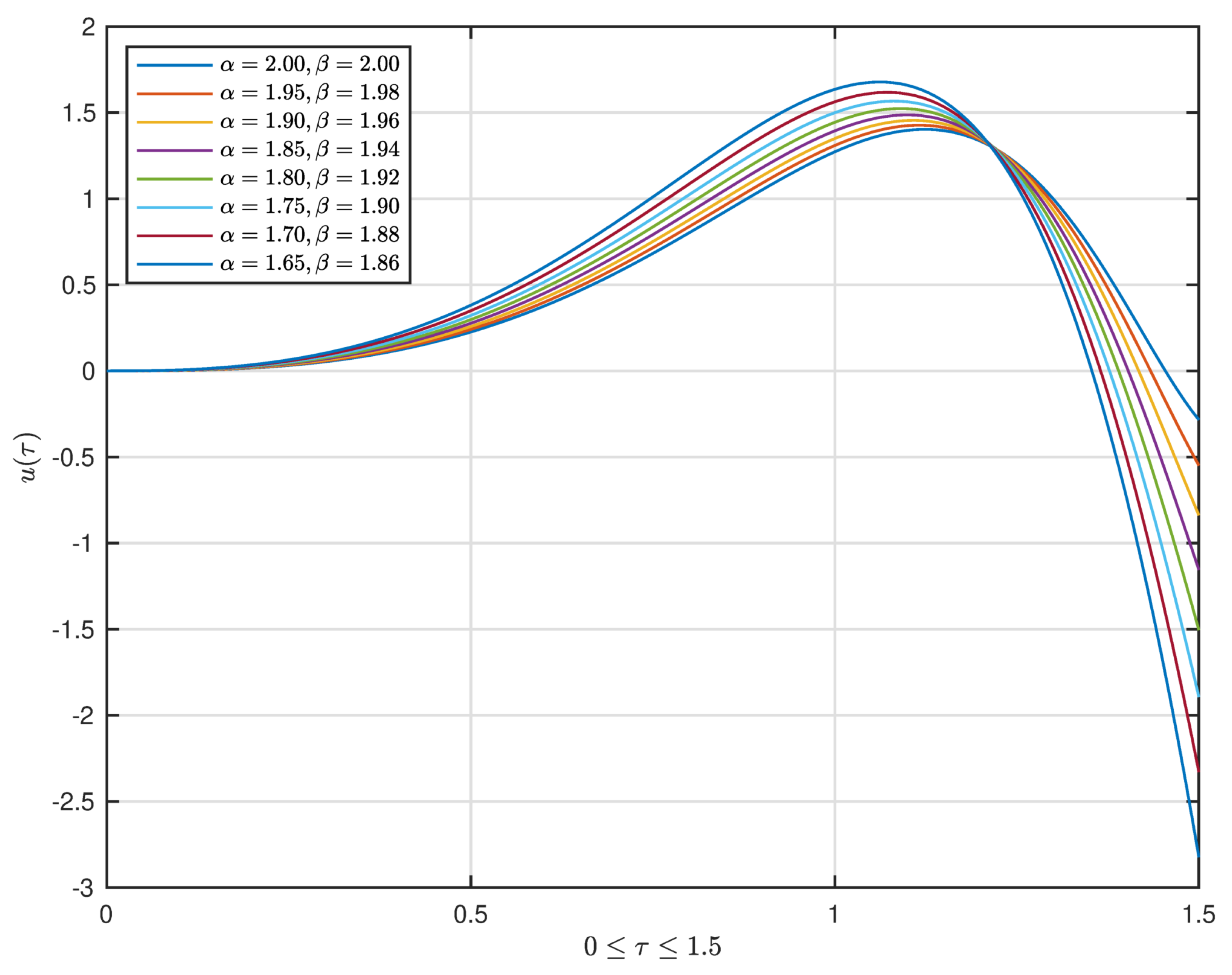We consider $f(\tau ,u(\tau ),(\mathcal{K}u\left)\right(\tau ),(\mathcal{W}u\left)\right(\tau \left)\right)$, $\mathcal{H}(\zeta ,u(\zeta \left)\right)$, and $\mathcal{G}(\sigma ,u(\sigma \left)\right)$ as follows:

(i) 

Given the function

$$\begin{array}{ccc}\hfill f(\tau ,u(\tau ),(\mathcal{K}u\left)\right(\tau ),(\mathcal{W}u\left)\right(\tau \left)\right)& =& \frac{{\tau }^4+2{\tau }^2-6}{5{\tau }^2+3t+4}+\frac{5e^{-2\tau -1}}{4-{sin}^2\pi \tau }·\frac{\left|u\right(\tau \left)\right|}{5+\left|u\right(\tau \left)\right|}\hfill \\ & & +\frac{2\tau +6}{3^{5\tau +2}}\left[\frac{\left|\right(\mathcal{K}u\left)\right(\tau \left)\right|}{4+\left|\right(\mathcal{K}u\left)\right(\tau \left)\right|}+\frac{\left|\right(\mathcal{W}u\left)\right(\tau \left)\right)|}{5+\left|\right(\mathcal{W}u\left)\right(\tau \left)\right)|}\right],\hfill \\ \hfill \mathcal{H}(\zeta ,u\left(\zeta \right))=\frac{2}{6+\left|u\right(\xi \left)\right|},& & \mathcal{G}(\sigma ,u\left(\sigma \right))=\frac{2\left|u\right(\sigma \left)\right|}{4+5\left|u\right(\sigma \left)\right|},\hfill \end{array}$$

where

$$\begin{array}{ccc}\hfill \left(\mathcal{K}u\right)\left(\tau \right)& =& \frac{1}{\mathrm{\Gamma }\left(0.8\right)}{\int }_0^{\tau }{\left(\psi \left(\tau \right)-\psi \left(s\right)\right)}^{0.8-1}{\psi }^{\prime }\left(s\right)k(\tau ,s)u\left(s\right)ds,\hfill \end{array}$$

(62)

$$\begin{array}{ccc}\hfill \left(\mathcal{W}u\right)\left(\tau \right)& =& \frac{1}{\mathrm{\Gamma }\left(1.7\right)}{\int }_0^{\tau }{\left(\psi \left(\tau \right)-\psi \left(s\right)\right)}^{1.7-1}{\psi }^{\prime }\left(s\right)w(\tau ,s)u\left(s\right)ds,\hfill \end{array}$$

(63)

with

$$k(\tau ,s)=\frac{2sin\left(\pi \tau \right)}{s^2+2\tau +5},w(\tau ,s)=\frac{3(2\tau -2)}{5+cos\left(\pi s\right)}.$$

For $u_i$, $v_i$, $w_i\in \mathbb{R}$, $i=1,2$, $\tau \in [0,3/2]$, we obtain

$$\begin{array}{ccc}& & \left|f(\tau ,u_1,v_1,w_1)-f(\tau ,u_2,v_2,w_2)\right|\le \frac{1}{3}|u_1-u_2|+\frac{1}{4}|v_1-v_2|+\frac{1}{5}|w_1-w_2|,\hfill \\ & & \left|\mathcal{H}(\tau ,u_1)-\mathcal{H}(\tau ,u_2)\right|\le \frac{1}{3}|u_1-u_2|\mathrm{and}\left|\mathcal{G}(\tau ,u_1)-\mathcal{G}(\tau ,u_2)\right|\le \frac{1}{2}|u_1-u_2|.\hfill \end{array}$$

The conditions $\left({\mathcal{P}}_1\right)$–$\left({\mathcal{P}}_2\right)$ are satisfied with ${\mathcal{L}}_1=1/3$, ${\mathcal{L}}_2=1/4$, ${\mathcal{L}}_3=1/5$, ${\mathcal{H}}_1^{*}=1/3$, ${\mathcal{G}}_1^{*}=1/2$, $k_1^{*}=2/5$, and $w_1^{*}=3/5$. Hence, ${\Delta }_1+{\Delta }_2\approx 0.6077104343<1$. Since, Theorem 1 are fulfilled. Then, the problem (61) has a unique solution on $[0,3/2]$. Moreover, we have

$${\mathfrak{C}}_f:=\frac{\mathrm{\Lambda }(\alpha +\beta )}{1-\left({\mathcal{L}}_1{\mathrm{\Psi }}^{\alpha +\beta }\left(b\right)+{\mathcal{L}}_2{k}_1^{*}{\mathrm{\Psi }}^{\theta +\alpha +\beta }\left(b\right)+{\mathcal{L}}_3{w}_1^{*}{\mathrm{\Psi }}^{\delta +\alpha +\beta }\left(b\right)\right)}\approx 0.55937654>0.$$

From Theorem 4, the problem (61) is $\mathbb{UH}$ and $\mathbb{GUH}$ stables on $[0,3/2]$. Take $\mathcal{T}\left(\tau \right)={(\psi \left(\tau \right)-\psi \left(0\right))}^{1/3}$, and we have

$${\mathcal{I}}_{a^{+}}^{\alpha ;\psi }\mathcal{T}\left(\tau \right)=\frac{\mathrm{\Gamma }(4/3)}{\mathrm{\Gamma }(17/6)}{(\psi \left(\tau \right)-\psi \left(0\right))}^{3/2}\mathcal{T}\left(\tau \right)\le \frac{\mathrm{\Gamma }(4/3){tan}^{3/2}(\pi /3)}{2\sqrt{2}\mathrm{\Gamma }(17/6)}\mathcal{T}\left(\tau \right).$$

The inequality (52) is fulfilled with ${\lambda }_{\mathcal{T}}=\frac{\mathrm{\Gamma }(4/3){tan}^{3/2}(\pi /3)}{2\sqrt{2}\mathrm{\Gamma }(17/6)}>0$ and $\Theta \approx 4.6986661$. Then,

$${\mathfrak{C}}_{f,\mathcal{T}}=\frac{\Theta {\lambda }_{\mathcal{T}}}{1-\left({\mathcal{L}}_1{\mathrm{\Psi }}^{\alpha +\beta }\left(b\right)+{\mathcal{L}}_2{k}_1^{*}{\mathrm{\Psi }}^{\theta +\alpha +\beta }\left(b\right)+{\mathcal{L}}_3{w}_1^{*}{\mathrm{\Psi }}^{\delta +\alpha +\beta }\left(b\right)\right)}\approx 2.08782437>0.$$

Therefore, from Theorem 5, the problem (61) is $\mathbb{UHR}$ and $\mathbb{GUHR}$ stables on $[0,3/2]$.

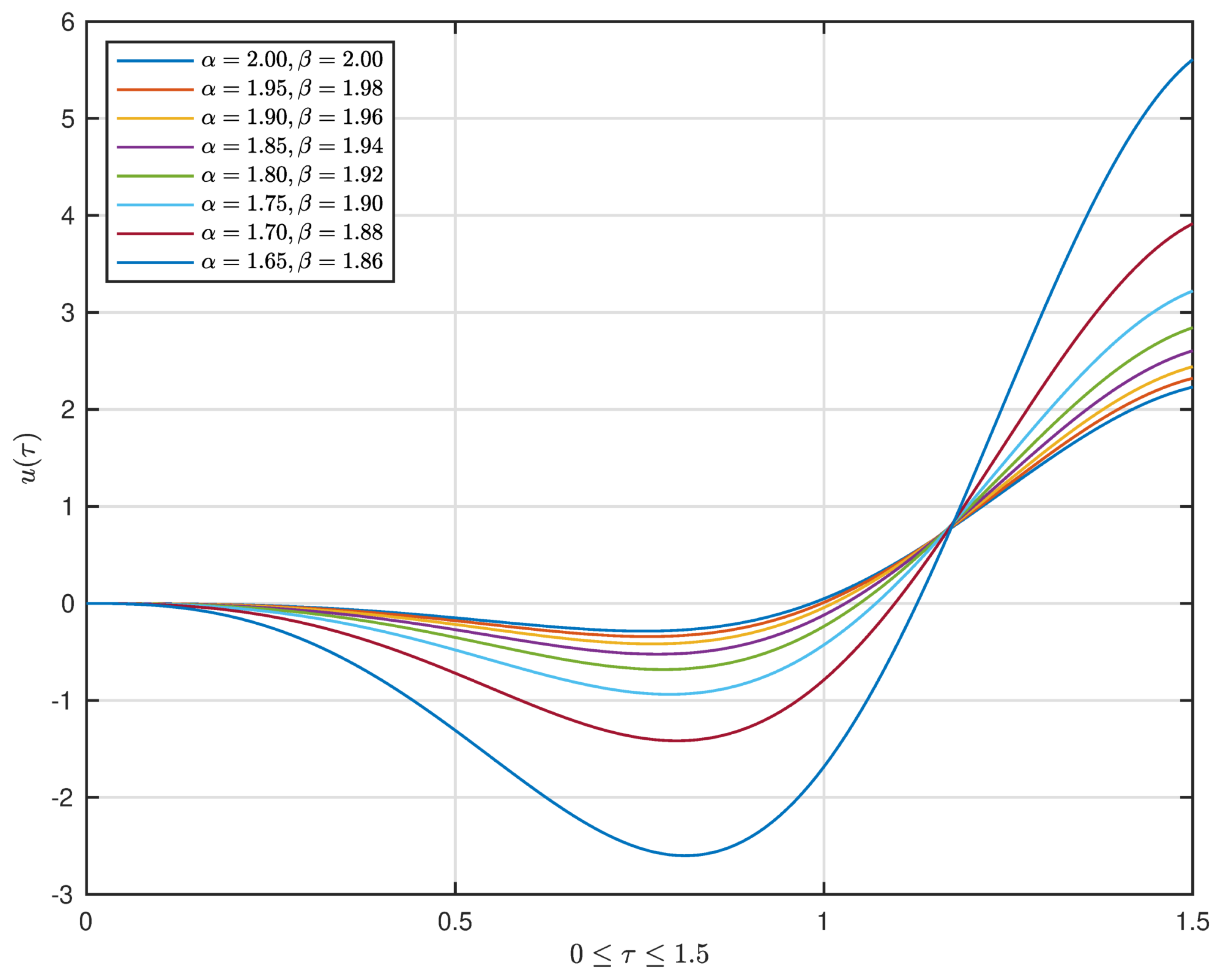
(ii) 

Given the function

$$\begin{array}{ccc}& & f(\tau ,u\left(\tau \right),\left(\mathcal{K}u\right)\left(\tau \right),\left(\mathcal{W}u\right)\left(\tau \right))=\frac{2cos\left(\pi \tau \right)+1}{3^{sin\left(\pi \tau \right)+2}}·\frac{\left|u\right(\tau \left)\right|+3}{2+\left|u\right(\tau \left)\right|}\hfill \\ & & +\frac{4\tau -1}{5^{3\tau +2}}·\left[\frac{\left|\right(\mathcal{K}u\left)\right(\tau \left)\right|+\left|\right(\mathcal{W}u\left)\right(\tau \left)\right|}{4+\left|\right(\mathcal{K}u\left)\right(\tau \left)\right|+\left|\right(\mathcal{W}u\left)\right(\tau \left)\right|}\right],\hfill \\ & & \mathcal{H}(\tau ,u\left(\tau \right))=\frac{4\tau +2}{5-2\tau }·\frac{\left|u\right(\tau \left)\right|}{8+5\left|u\right(\tau \left)\right|},\mathcal{G}(\tau ,u\left(\tau \right))=\frac{\tau sin\left(u\right(\tau \left)\right)}{9},\hfill \end{array}$$

with (62) and (63), where $k(\tau ,s)=2/(5+s^{\tau +1})$ and $w(\tau ,s)=3/(7-2sin(\pi s\tau \left)\right)$.

For u, v, $w\in \mathbb{R}$, and $\tau \in [0,3/2]$, we estimate that

$$\begin{array}{ccc}& & \left|f(\tau ,u,v,w)\right|\le \frac{1+2cos\left(\pi \tau \right)}{3^{sin\left(\pi \tau \right)+2}}·\frac{\left|u\right(\tau \left)\right|+3}{2}+\frac{4\tau -1}{5^{3\tau +2}}·\frac{\left|v\right|+\left|w\right|}{4}\hfill \\ & & \left|\mathcal{H}(\tau ,u)\right|\le \frac{4\tau +2}{5-2\tau }·\frac{\left|u\right|}{8},\left|\mathcal{G}(\tau ,u)\right|\le \frac{\tau }{9}·\left|u\right|.\hfill \end{array}$$

The assumption $\left({\mathcal{P}}_4\right)$ is also valid with $p_1\left(\tau \right)=(1+2cos\left(\pi \tau \right))/\left(3^{sin\left(\pi \tau \right)+2}\right)$, $p_2\left(\tau \right)=(4\tau -1)/(4·5^{3\tau +2})=p_3\left(\tau \right)$, $q_1\left(\tau \right)=(4\tau +2)/(5-2\tau )$, $q_2\left(\tau \right)=\tau /9$, $\mathbb{U}\left(\right|u\left|\right)=\left(\right|u|+3)/2$, $\mathbb{V}\left(\right|u\left|\right)=\left|u\right|/8$ and $\mathbb{W}\left(\right|u\left|\right)=\left|u\right|$. Thus, $p_1^{*}=1/3$, $p_2^{*}=1/20=p_3^{*}$, $q_1^{*}=4$, $q_2^{*}=1/6$, $k_1^{*}=2/5$, and $w_1^{*}=3/5$. There is a positive constant ${\mathcal{M}}^{*}>0.37949755$ verifying (${\mathcal{P}}_5$). Then, Theorem is fulfilled, and we can summarize that the problem (61) has at least one solution on $[0,3/2]$.

For any $u_i$, $v_i$, $w_i\in \mathbb{R}$, $i=1,2,$ and $\tau \in [0,3/2]$, one has

$$\left|f(\tau ,u_1,v_1,w_1)-f(\tau ,u_2,v_2,w_2)\right|\le \frac{5}{12}\left|u_1-u_2\right|+\frac{1}{20}\left|v_1-v_2\right|+\frac{1}{20}\left|w_1-w_2\right|.$$

The conditions $\left({\mathcal{P}}_1\right)$-$\left({\mathcal{P}}_2\right)$ are verified with ${\mathcal{L}}_1=5/12$, ${\mathcal{L}}_2={\mathcal{L}}_3=1/20$, ${\mathcal{H}}_1^{*}=1/2$, ${\mathcal{G}}_1^{*}=1/6$, $k_1^{*}=2/5$ and $w_1^{*}=3/5$. Thus, ${\Delta }_1+{\Delta }_2\approx 0.44078217<1$. Hence, the problem (61) has a unique solution on $[0,3/2]$. Moreover, we obtain ${\mathfrak{C}}_f:=0.56437711>0$. Theorem 4 is satisfied, the problem (61) is $\mathbb{UH}$ and $\mathbb{GUH}$ stables on $[0,3/2]$. Take $\mathcal{T}\left(\tau \right)={(\psi \left(\tau \right)-\psi \left(0\right))}^{1/2}$, and we have

$${\mathcal{I}}_{a^{+}}^{\alpha ;\psi }\mathcal{T}\left(\tau \right)=\frac{1}{4\sqrt{\pi }}{(\psi \left(t\right)-\psi \left(0\right))}^{3/2}\mathcal{T}\left(\tau \right)\le \frac{{tan}^{3/2}(\pi /3)}{8\sqrt{2\pi }}\mathcal{T}\left(\tau \right).$$

The inequality (52) is satisfied with ${\lambda }_{\mathcal{T}}=\frac{{tan}^{3/2}(\pi /3)}{8\sqrt{2\pi }}>0$ and $\Theta \approx 4.69866612$. Then,

$${\mathfrak{C}}_{f,\mathcal{T}}=\frac{\Theta {\lambda }_{\mathcal{T}}}{1-\left({\mathcal{L}}_1{\mathrm{\Psi }}^{\alpha +\beta }\left(b\right)+{\mathcal{L}}_2{k}_1^{*}{\mathrm{\Psi }}^{\theta +\alpha +\beta }\left(b\right)+{\mathcal{L}}_3{w}_1^{*}{\mathrm{\Psi }}^{\delta +\alpha +\beta }\left(b\right)\right)}\approx 2.10648855>0.$$

Hence, Theorem 5 is true, and the problem (61) is $\mathbb{UHR}$ and $\mathbb{GUHR}$ stables on $[0,3/2]$.

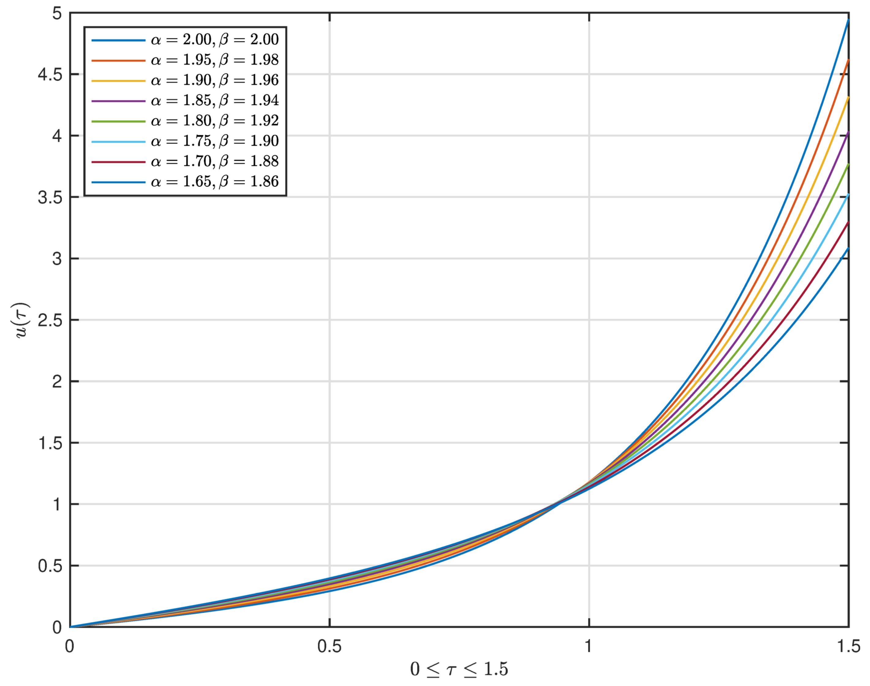
(iii) 

Given the function

$$\begin{array}{ccc}& & f(\tau ,u\left(\tau \right),\left(\mathcal{K}u\right)\left(\tau \right),\left(\mathcal{W}u\right)\left(\tau \right))=\frac{e^{3\tau -5}}{ln(5-2\tau )}+\frac{\sqrt{4{\tau }^2+2\tau +4}}{\tau sin\left(\tau \right)+6}sin\left(u\left(\tau \right)\right)\hfill \\ & & +\frac{2\tau }{9-2\tau }·\frac{\left|\right(\mathcal{K}u\left)\right(\tau \left)\right|}{1+2\left|\right(\mathcal{K}u\left)\right(\tau \left)\right|}\hfill \\ & & +\frac{4cos\tau }{3^{6\tau +2}}arctan\left(\left(\mathcal{W}u\right)\left(\tau \right)\right),\hfill \\ & & \mathcal{H}(\tau ,u\left(\tau \right))=\frac{\left|2u\right(\tau )+5|}{{\tau }^2+5},\mathcal{G}(\tau ,u\left(\tau \right))=\frac{2\tau sin\left(u\right(\tau \left)\right)+3}{5+ln(2\tau +5)},\hfill \end{array}$$

with (62) and (63), where $k(\tau ,s)=4/(7+s\tau )$ and $w(\tau ,s)=2/(7+2s{cos}^2\left(\pi \tau \right))$.

For any $u_i$, $v_i$, $w_i\in \mathbb{R}$, $i=1,2$, and $\tau \in [0,3/2]$, we obtain

$$\begin{array}{ccc}& & \left|f(\tau ,u_1,v_1,w_1)-f(\tau ,u_2,v_2,w_2)\right|\le \frac{2}{3}|u_1-u_2|+\frac{1}{2}|v_1-v_2|+\frac{4}{9}|w_1-w_2|,\hfill \\ & & \left|\mathcal{H}(\tau ,u_1)-\mathcal{H}(\tau ,u_2)\right|\le \frac{2}{5}|u_1-u_2|\mathrm{and}\left|\mathcal{G}(\tau ,u_1)-\mathcal{G}(\tau ,u_2)\right|\le \frac{3}{5}|u_1-u_2|.\hfill \end{array}$$

The conditions $\left({\mathcal{P}}_1\right)$-$\left({\mathcal{P}}_2\right)$ are satisfied with ${\mathcal{L}}_1=2/3$, ${\mathcal{L}}_2=1/2$, ${\mathcal{L}}_3=4/9$, ${\mathcal{H}}_1^{*}=2/5$, ${\mathcal{G}}_1^{*}=3/5$, $k_1^{*}=4/7$, and $w_1^{*}=2/7$. Hence, we have

$$\left({\Delta }_1+{\Delta }_2-{\mathrm{\Psi }}^{\alpha +\beta }\left(b\right){\mathcal{L}}_1-{\mathrm{\Psi }}^{\theta +\alpha +\beta }\left(b\right)k_1^{*}{\mathcal{L}}_2-{\mathrm{\Psi }}^{\delta +\alpha +\beta }\left(b\right)w_1^{*}{\mathcal{L}}_3\right)\approx 0.76735591<1.$$

For u, v, $w\in \mathbb{R}$, and $\tau \in [0,3/2]$, we have

$$\begin{array}{ccc}& & \left|f(\tau ,u,v,w)\right|\le \frac{e^{3\tau -5}}{ln(5-2\tau )}+\frac{\sqrt{4{\tau }^2+2\tau +4}}{\tau sin\left(\tau \right)+6}\left|u\left(\tau \right)\right|\hfill \\ & & +\frac{2\tau }{9-2\tau }\left|\left(\mathcal{K}u\right)\left(\tau \right)\right|+\frac{4cos\tau }{3^{6\tau +2}}\left|\left(\mathcal{W}u\right)\left(\tau \right)\right|,\hfill \\ & & \left|\mathcal{H}(\tau ,u)\right|\le \frac{2\left|u\right|}{{\tau }^2+5}+\frac{5}{{\tau }^2+5},\left|\mathcal{G}(\tau ,u)\right|\le \frac{2\tau \left|u\right|}{5+ln(2\tau +5)}+\frac{3}{5+ln(2\tau +5)}.\hfill \end{array}$$

The condition $\left({\mathcal{P}}_5\right)$ is verified with $f_1\left(\tau \right)=e^{3\tau -5}/ln(5-2\tau )$, $f_2\left(\tau \right)=\sqrt{4{\tau }^2+2\tau +4}$$/(\tau sin(\tau )+6)$, $f_3\left(\tau \right)=2\tau /(9-2\tau )$, $f_4\left(\tau \right)=4cos\tau /3^{6\tau +2}$, $h_1\left(\tau \right)=5/({\tau }^2+5)$, $h_2\left(\tau \right)=2/({\tau }^2+5)$, $g_1\left(\tau \right)=3/(5+ln(2\tau +5)$, and $g_2\left(\tau \right)=2\tau /(5+ln(2\tau +5))$. So, Theorem 3 is verified, and we can summarize that the problem (61) has at least one solution on $[0,3/2]$.

In addition, the problem (61) has a unique solution on $[0,3/2]$ with ${\Delta }_1+{\Delta }_2\approx 0.89211721<1$. Moreover, we have that ${\mathfrak{C}}_f:=0.60023816>0$. Then, Theorem 4 is true, and the problem (61) is $\mathbb{UH}$ and $\mathbb{GUH}$ stables on $[0,3/2]$. Take $\mathcal{T}\left(\tau \right)={(\psi \left(\tau \right)-\psi \left(0\right))}^{1/4}$, and we get ${\lambda }_{\mathcal{T}}=\frac{\mathrm{\Gamma }(5/4){tan}^{3/2}(\pi /3)}{2\sqrt{2}\mathrm{\Gamma }(11/4)}\approx 0.45418619>0$ and $\Theta \approx 4.69866612$. Then, we obtain ${\mathfrak{C}}_{f,\mathcal{T}}\approx 2.43827113>0$. From Theorem 5, then, the problem (61), is $\mathbb{UHR}$ and $\mathbb{GUHR}$ stables on $[0,3/2]$.

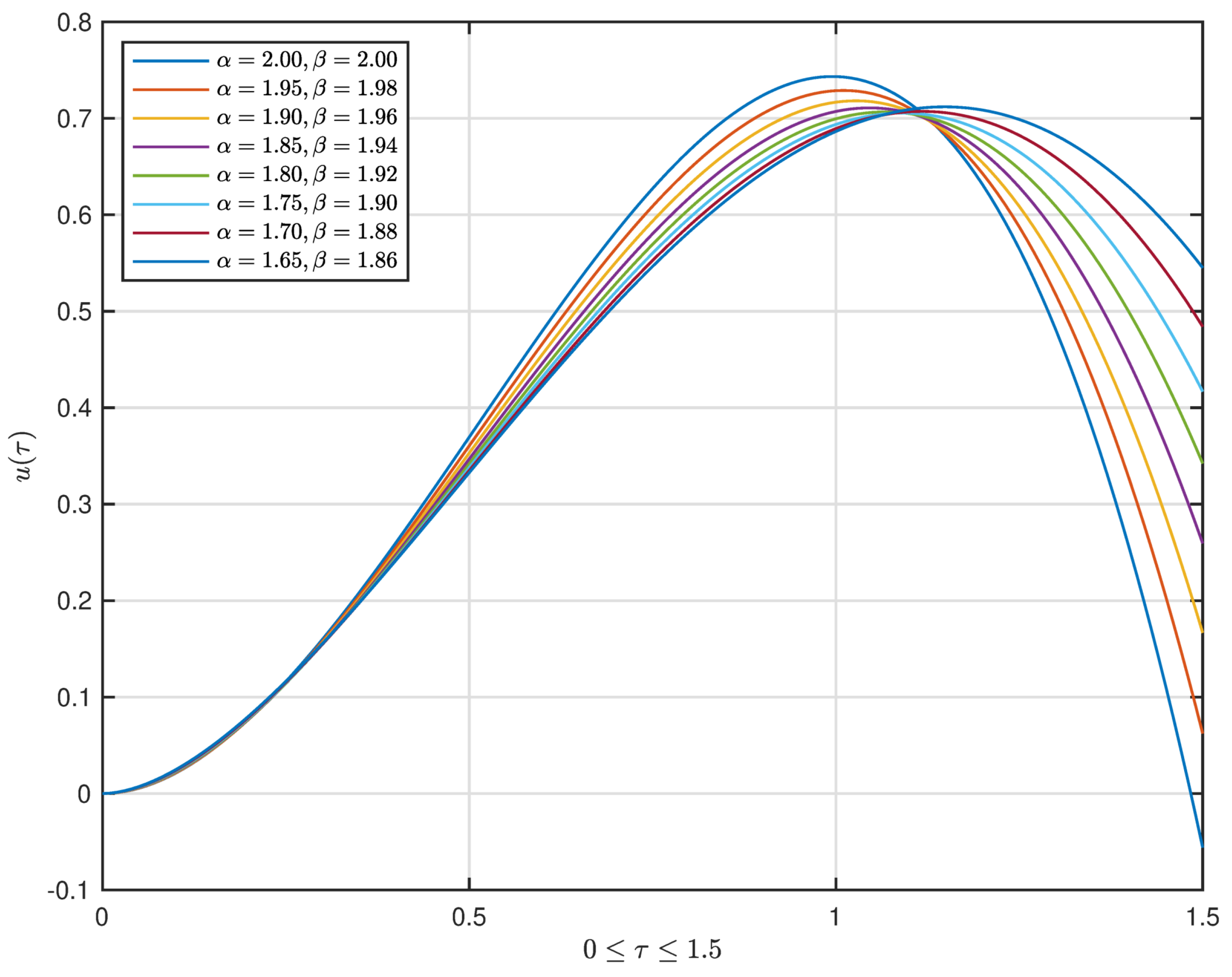
(iv) 

Consider $f(\tau ,u\left(\tau \right),\left(\mathcal{K}u\right)\left(\tau \right),\left(\mathcal{W}u\right)\left(\tau \right))={\varrho }_1{\left(\psi \left(\tau \right)-\psi \left(0\right)\right)}^{{\varpi }_1}$ and

$$\mathcal{G}(\tau ,u\left(\tau \right))={\varrho }_2{\left(\psi \left(\tau \right)-\psi \left(0\right)\right)}^{{\varpi }_2},\mathcal{H}(\tau ,u\left(\tau \right))={\varrho }_3{\left(\psi \left(\tau \right)-\psi \left(0\right)\right)}^{{\varpi }_3}.$$

By Lemma 4 with ${\varrho }_1=2$, ${\varrho }_2=3$, ${\varrho }_3=4$, ${\varpi }_1=1/7$, ${\varpi }_2=1/5$, and ${\varpi }_3=1/3$, the solution of the problem (61) is given by

$$\begin{array}{ccc}& & x\left(\tau \right)\hfill \\ & =& \frac{2\mathrm{\Gamma }(8/7){\left(\psi \left(\tau \right)-\psi \left(0\right)\right)}^{1/7+\alpha +\beta }}{\mathrm{\Gamma }(8/7+\alpha +\beta )}+\frac{{\left(\psi \left(\tau \right)-\psi \left(0\right)\right)}^{{\gamma }_1+\beta -1}}{\mathrm{\Omega }\mathrm{\Gamma }({\gamma }_1+\beta )}\hfill \\ & & \times [{\mathrm{\Omega }}_{22}\left(\frac{3\mathrm{\Gamma }(6/5){\left(\psi \left(\sigma \right)-\psi \left(0\right)\right)}^{7/5}}{\mathrm{\Gamma }(12/5)}-\sum _{i=1}^m\frac{2\mathrm{\Gamma }(8/7){\xi }_i{\left(\psi \left({\eta }_i\right)-\psi \left(0\right)\right)}^{1/7+\alpha +\beta }}{\mathrm{\Gamma }(8/7+\alpha +\beta )}\right)\hfill \\ & & -{\mathrm{\Omega }}_{12}\left(\frac{4\mathrm{\Gamma }(4/3){\left(\psi \left(\zeta \right)-\psi \left(0\right)\right)}^{11/6}}{\mathrm{\Gamma }(17/6)}-\sum _{j=1}^n\frac{2\mathrm{\Gamma }(8/7){\mu }_j{\left(\psi \left({\lambda }_j\right)-\psi \left(0\right)\right)}^{1/7+\alpha +\beta -{\varphi }_j}}{\mathrm{\Gamma }(8/7+\alpha +\beta -{\varphi }_j)}\right)]\hfill \\ & & +\frac{{\left(\psi \left(t\right)-\psi \left(0\right)\right)}^{{\gamma }_2-1}}{\mathrm{\Omega }\mathrm{\Gamma }\left({\gamma }_2\right)}\left[{\mathrm{\Omega }}_{11}\right(\frac{4\mathrm{\Gamma }(4/3){\left(\psi \left(\zeta \right)-\psi \left(0\right)\right)}^{11/6}}{\mathrm{\Gamma }(17/6)}\hfill \\ & & -\sum _{j=1}^n\frac{2\mathrm{\Gamma }(8/7){\mu }_j{\left(\psi \left({\lambda }_j\right)-\psi \left(0\right)\right)}^{1/7+\alpha +\beta -{\varphi }_j}}{\mathrm{\Gamma }(8/7+\alpha +\beta -{\varphi }_j)})\hfill \\ & & -{\mathrm{\Omega }}_{21}\left(\frac{3\mathrm{\Gamma }(6/5){\left(\psi \left(\sigma \right)-\psi \left(0\right)\right)}^{7/5}}{\mathrm{\Gamma }(12/5)}-\sum _{i=1}^m\frac{2\mathrm{\Gamma }(8/7){\xi }_i{\left(\psi \left({\eta }_i\right)-\psi \left(0\right)\right)}^{1/7+\alpha +\beta }}{\mathrm{\Gamma }(8/7+\alpha +\beta )}\right)].\hfill \end{array}$$

A graph displaying of $u\left(\tau \right)$ for the problem (61) under $\alpha =1.65,1.70,\dots ,2.00$ and $\beta =1.86,1.88,\dots ,2.00$ with $\psi \left(\tau \right)={\tau }^{\sqrt{\alpha }+\sqrt{\beta }}$, ${(sin\tau )}^{\sqrt{\alpha }+\sqrt{\beta }}$, ${(\alpha +\beta )}^{\frac{\tau }{2}}$, ${(ln(\tau +1))}^{\sqrt{\alpha +\beta }}$, is shown in Figure 1, Figure 2, Figure 3 and Figure 4.

6. Conclusions

The main aims of this study have been accomplished. Firstly, the uniqueness result for a nonlinear $\psi$-Hilfer $\mathbb{FBVP}$ describing Navier model with $\mathbb{NIBC}$s was analyzed by helping Banach’s fixed point theorem. Afterward, the existence results were established by applying fixed point theory of Leray-Schauder’s and Kransnoselskii’s types, while the guarantee of the existence of solutions was shown by the powerful techniques, such as Ulam’s stability, including $\mathbb{UH}$, $\mathbb{GUH}$, $\mathbb{UHR}$, and $\mathbb{GUHR}$ stables. Finally, we ensured the theoretical results via some illustrates in the special cases of $\psi$ are polynomial, trigonometry, exponential, and logarithm functions. This paper has considered different methods and is attractive for researchers who are interested in the work of the integro-differential equation describing Navier model under $\psi$-Hilfer fractional operators. We will concentrate on examining the qualitative theories of solutions to nonlinear equations or systems of real-world models with boundary conditions in the context of other fractional calculus in the future. It also remains to extend the results obtained to new Hilfer-type operators; see, for example, Reference [59].

References

- Podlubny, I. Fractional Differential Equations; Academic Press: New York, NY, USA, 1999. [Google Scholar]
- Hilfer, R. Applications of Fractional Calculus in Physics; World Scientific: Singapore, 2000. [Google Scholar]
- Kilbas, A.A.; Srivastava, H.M.; Trujillo, J.J. Theory and Applications of Fractional Differential Equations; Elsevier Science: Amsterdam, The Netherlands, 2006. [Google Scholar]
- Nandal, S.; Zaky, M.A.; De Staelen, R.H.; Hendy, A.S. Numerical simulation for a multidimensional fourth-order nonlinear fractional subdiffusion model with time delay. Mathematics 2021, 9, 3050. [Google Scholar] [CrossRef]
- Shokri, A. An explicit trigonometrically fitted ten-step method with phase-lag of order infinity for the numerical solution of the radial Schrödinger equation. Appl. Comput. Math. 2015, 14, 63–74. [Google Scholar]
- Baleanu, D.; Mousalou, A.; Rezapour, S. On the existence of solutions for some infinite coefficient-symmetric Caputo-Fabrizio fractional integro-differential equations. Bound. Value Probl. 2017, 207, 145. [Google Scholar] [CrossRef]
- Hao, X.; Sun, H.; Liu, L. Existence results for fractional integral boundary value problem involving fractional derivatives on an infinite interval. Math. Methods Appl. Sci. 2018, 41, 6984–6996. [Google Scholar] [CrossRef]
- Harikrishman, S.; Elsayed, E.; Kanagarajan, K. Existence and uniqueness results for fractional pantograph equations involving ψ-Hilfer fractional derivative. Dyn. Contin. Discrete Impuls. Syst. Ser. A Math. Anal. 2018, 25, 319–328. [Google Scholar]
- Boutiara, A.; Guerbati, K.; Benbachir, M. Caputo-Hadamard fractional differential equation with three-point boundary conditions in Banach spaces. AIMS Math. 2020, 5, 259–272. [Google Scholar]
- Ahmed, I.; Kuman, P.; Shah, K.; Borisut, P.; Sitthithakerngkiet, K.; Demba, M.A. Stability results for implicit fractional pantograph differential equations via ψ-Hilfer fractional derivative with a nonlocal Riemann-Liouville fractional integral condition. Mathematics 2020, 8, 94. [Google Scholar] [CrossRef] [Green Version]
- Etemad, S.; Ntouyas, S.K.; Imran, A.; Hussain, A.; Baleanu, D.; Rezapour, S. Application of some special operators on theanalysis of a new generalized fractional Navier problem in the context of q-calculus. Adv. Differ. Equ. 2021, 2021, 402. [Google Scholar] [CrossRef]
- Rezapour, S.; Tellab, B.; Deressa, C.T.; Etemad, S.; Nonlaopon, K. H-U-Type Stability and numerical solutions for a nonlinear model of the coupled systems of Navier BVPs via the generalized differential transform method. Fractal Fract. 2021, 5, 166. [Google Scholar] [CrossRef]
- Karthikeyan, K.; Karthikeyan, P.; Patanarapeelert, N.; Sitthiwirattham, T. Mild Solutions for Impulsive Integro-Differential Equations Involving Hilfer Fractional Derivative with almost Sectorial Operators. Axioms 2021, 10, 313. [Google Scholar] [CrossRef]
- Ahmad, B.; Ntouyas, S.K. Hilfer-Hadamard fractional boundary value problems with nonlocal mixed boundary conditions. Fractal Fract. 2021, 5, 195. [Google Scholar] [CrossRef]
- Shokri, A. The symmetric two-step P-stable nonlinear predictor-corrector methods for the numerical solution of second order initial value problems. Bull. Iran. Math. Soc. 2015, 41, 201–215. [Google Scholar]
- Saeed, A.M.; Abdo, M.S.; Jeelani, M.B. Existence and Ulam-Hyers stability of a fractional-order coupled system in the frame of generalized Hilfer derivatives. Mathematics 2021, 9, 2543. [Google Scholar] [CrossRef]
- Karthikeyan, K.; Karthikeyan, P.; Chalishajar, D.N.; Raja, D.S.; Sundararajan, P. Analysis on ψ-Hilfer fractional impulsive differential equations. Symmetry 2021, 13, 1895. [Google Scholar] [CrossRef]
- Boutiara, A.; Abdo, M.S.; Almalahi, M.A.; Ahmad, H.; Ishan, A. Implicit hybrid fractional boundary value problem via generalized Hilfer derivative. Symmetry 2021, 13, 1937. [Google Scholar] [CrossRef]
- Kotsamran, K.; Sudsutad, W.; Thaiprayoon, C.; Kongson, J.; Alzabut, J. Analysis of a nonlinear ψ-Hilfer fractional integro-differential equation describing cantilever beam model with nonlinear boundary conditions. Fractal Fract. 2021, 5, 177. [Google Scholar] [CrossRef]
- Gupta, C.P. Existence and uniqueness theorems for the bending of an elastic beam equation. Appl. Anal. 1988, 26, 289–304. [Google Scholar] [CrossRef]
- Zhong, Y.; Chen, S.; Wang, C. Existence results for a fourth-order ordinary differential equation with a four-point boundary condition. Appl. Math. Lett. 2008, 21, 465–470. [Google Scholar] [CrossRef] [Green Version]
- Sun, J.P.; Wang, X.Y. Positive solution for fourth-order four-point Sturm-Liouville boundary value problem. J. Appl. Math. Inform. 2010, 28, 679–686. [Google Scholar]
- Bonanno, G.; Chinni, A.; Tersian, S.A. Existence results for a two point boundary value problem involving a fourth-order equation. Electron. J. Qual. Theory Differ. Equ. 2015, 33, 1–9. [Google Scholar] [CrossRef]
- Bouteraa, N.; Benaicha, S.; Djourdem, H.; Benattia, M.E. Positive solutions of nonlinear fourth-order two-point boundary value problem with a parameter. Rom. J. Math. Comput. Sci. 2018, 8, 17–30. [Google Scholar]
- Tuz, M. The Existence of symmetric positive solutions of fourth-order elastic beam equations. Symmetry 2019, 11, 121. [Google Scholar] [CrossRef] [Green Version]
- Alzabut, J.; Selvam, A.G.M.; Dhineshbabu, R.; Kaabar, M.K.A. The existence, uniqueness, and stability analysis of the discrete fractional three-point boundary value problem for the elastic beam equation. Symmetry 2021, 13, 789. [Google Scholar] [CrossRef]
- Faraji Oskouie, M.; Ansari, R.; Rouhi, H. Bending analysis of functionally graded nanobeams based on the fractional nonlocal continuum theory by the variational Legendre spectral collocation method. Meccanica 2018, 53, 1115–1130. [Google Scholar] [CrossRef]
- Sidhardh, S.; Patnaik, S.; Semperlotti, F. Fractional-order structural stability: Formulation and application to the critical load of nonlocal slender structures. Int. J. Mech. Sci. 2021, 201, 106443. [Google Scholar] [CrossRef]
- Lazopoulos, K.A.; Lazopoulos, A.K. On the fractional deformation of a linearly elastic bar. J. Mech. Behav. Mater. 2020, 29, 9–18. [Google Scholar] [CrossRef]
- Lazopoulos, K.A.; Lazopoulos, A.K. On fractional bending of beams. Arch. Appl. Mech. 2016, 86, 1133–1145. [Google Scholar] [CrossRef]
- Alotta, G.; Failla, G.; Zingales, M. Finite element formulation of a nonlocal hereditary fractional-order timoshenko beam. J. Eng. Mech. 2015, 143, D4015001. [Google Scholar] [CrossRef]
- Tarasov, V.E. Fractional mechanics of elastic solids: Continuum aspects. J. Eng. Mech. 2016, 143, D4016001. [Google Scholar] [CrossRef]
- Failla, G. Stationary response of beams and frames with fractional dampers through exact frequency response functions. J. Eng. Mech.-A Solids 2016, 143, D4016004. [Google Scholar] [CrossRef]
- Sumelka, W.; Blaszczyk, T.; Liebold, C. Fractional Euler-Bernoulli beams: Theory, numerical study and experimental validation. Eur. J. Mech. 2015, 54, 243–251. [Google Scholar] [CrossRef] [Green Version]
- Sidhardh, S.; Patnaik, S.; Semperlotti, F. Geometrically nonlinear response of a fractional-order nonlocal model of elasticity. Int. J.-Non Mech. 2020, 125, 103529. [Google Scholar] [CrossRef]
- Stempin, P.; Sumelka, W. Space-Fractional Euler-Bernoulli beam model theory and identification for silver nanobeam bending. Int. J. Mech. Sci. 2020, 186, 105902. [Google Scholar] [CrossRef]
- Reiss, E.L.; Callegari, A.J.; Ahluwalia, D.S. Ordinary Differential Equations with Applications; Holt, Rinehart & Winston: New York, NY, USA, 1978. [Google Scholar]
- Aftabizadeh, A.R. Existence and uniqueness theorems for fourth-order boundary value problems. J. Math. Anal. Appl. 1986, 116, 415–426. [Google Scholar] [CrossRef] [Green Version]
- Ma, R.; Zhang, J.; Fu, S. The method of lower and upper solutions for fourth-order two-point boundary value problems. J. Math. Anal. Appl. 1997, 215, 415–422. [Google Scholar]
- Bai, Z.; Ge, W.; Wang, Y. The method of lower and upper solutions for some fourth-order equations. J. Inequal. Pure Appl. Math. 2004, 5, 13. [Google Scholar]
- Dang, Q.A.; Long, D.Q.; Ngo, T.K.Q. A novel efficient method for nonlinear boundary value problems. Numer. Algorithms 2017, 76, 427–439. [Google Scholar] [CrossRef]
- Bachar, I.; Eltayeb, H. Existence and uniqueness results for fractional Navier boundary value problems. Adv. Differ. Equ. 2020, 2020, 609. [Google Scholar] [CrossRef]
- Abdeljawad, T.; Karapınar, E.; Panda, S.K.; Mlaiki, N. Solutions of boundary value problems on extended-Branciari b-distance. J. Inequa. Appl. 2020, 2020, 103. [Google Scholar] [CrossRef]
- Chandran, K.; Gopalan, K.; Zubair, S.T.; Abdeljawad, T. A fixed point approach to the solution of singular fractional differential equations with integral boundary conditions. Adv. Differ. Equ. 2021, 2021, 56. [Google Scholar] [CrossRef]
- Etemad, S.; Rezapour, S. On the existence of solutions for fractional boundary value problems on the ethane graph. Adv. Differ. Equ. 2020, 2020, 276. [Google Scholar] [CrossRef]
- Tarasov, V.E. Fractional integro-differential equations for electromagnetic waves in dielectric media. Theor. Math. Phys. 2009, 158, 355–359. [Google Scholar] [CrossRef] [Green Version]
- Yang, A.M.; Han, Y.; Zhang, Y.Z.; Wang, L.T.; Zhang, D.; Yang, X.J. On nonlocal fractional Volterra integro-differential equations in fractional steady heat transfer. Therm. Sci. 2016, 20, 789–793. [Google Scholar] [CrossRef] [Green Version]
- Sousa, J.V.D.C.; De Oliveira, E.C. Capelas de: Ulam-Hyers stability of a nonlinear fractional Volterra integro-differential equation. Appl. Math. Lett. 2018, 81, 50–56. [Google Scholar] [CrossRef]
- Zada, A.; Alzabut, J.; Waheed, H.; Popa, I.-L. Ulam-Hyers stability of impulsive integrodifferential equations with Riemann-Liouville boundary conditions. Adv. Differ. Equ. 2020, 2020, 64. [Google Scholar] [CrossRef] [Green Version]
- Sousa, J.; Vanterler da, C.; Oliveira, E. Capelas de: On the Ulam-Hyers-Rassias stability for nonlinear fractional differential equations using the ψ-Hilfer operator. J. Fixed Point Theory Appl. 2018, 20, 96. [Google Scholar] [CrossRef]
- Thaiprayoon, C.; Sudsutad, W.; Alzabut, J.; Etemad, S.; Rezapour, S. On the qualitative analysis of the fractional boundary value problem describing thermostat control model via ψ-Hilfer fractional operator. Adv. Differ. Equ. 2021, 2021, 201. [Google Scholar] [CrossRef]
- Alzabut, J.; Adjabi, Y.; Sudsutad, W.; Ur Rehman, M. New generalizations for Gronwall type inequalities involving a ψ-fractional operator and their applications. AIMS Math. 2021, 6, 5053–5077. [Google Scholar] [CrossRef]
- Seemab, A.; Ur Rehman, M.; Alzabut, J.; Adjabi, Y.; Abdo, M.S. Langevin equation with nonlocal boundary conditions involving a ψ-Caputo fractional operators of different orders. AIMS Math. 2021, 6, 6749–6780. [Google Scholar] [CrossRef]
- Shatanawi, W.; Boutiara, A.; Abdo, M.S.; Jeelani, M.B.; Abodayeh, K. Nonlocal and multiple point fractional boundary value problem in the frame of a generalized Hilfer derivative. Adv. Differ. Equ. 2021, 2021, 294. [Google Scholar] [CrossRef]
- Sousa, J.V.C.; Capelas de Oliveira, E. On the ψ-Hilfer fractional derivative. Commun. Nonlinear Sci. Numer. Simul. 2018, 60, 72–91. [Google Scholar] [CrossRef]
- Granas, A.; Dugundji, J. Fixed Point Theory; Springer: New York, NY, USA, 2003. [Google Scholar]
- Griffel, D.H. Applied Functional Analysis; Ellis Horwood: Chichester, UK, 1981. [Google Scholar]
- Krasnoselskii, M.A. Two remarks on the method of successive approximations. Usp. Mat. Nauk 1955, 10, 123–127. [Google Scholar]
- Valdés, J.E.N. Generalized fractional Hilfer integral and derivative. Contrib. Math. 2020, 2, 55–60. [Google Scholar] [CrossRef]
Publisher’s Note: MDPI stays neutral with regard to jurisdictional claims in published maps and institutional affiliations. |
© 2021 by the authors. Licensee MDPI, Basel, Switzerland. This article is an open access article distributed under the terms and conditions of the Creative Commons Attribution (CC BY) license (https://creativecommons.org/licenses/by/4.0/).
Share and Cite
Pleumpreedaporn, S.; Sudsutad, W.; Thaiprayoon, C.; Nápoles, J.E.; Kongson, J. A Study of ψ-Hilfer Fractional Boundary Value Problem via Nonlinear Integral Conditions Describing Navier Model. Mathematics 2021, 9, 3292. https://doi.org/10.3390/math9243292
Pleumpreedaporn S, Sudsutad W, Thaiprayoon C, Nápoles JE, Kongson J. A Study of ψ-Hilfer Fractional Boundary Value Problem via Nonlinear Integral Conditions Describing Navier Model. Mathematics. 2021; 9(24):3292. https://doi.org/10.3390/math9243292
Chicago/Turabian StylePleumpreedaporn, Songkran, Weerawat Sudsutad, Chatthai Thaiprayoon, Juan E. Nápoles, and Jutarat Kongson. 2021. "A Study of ψ-Hilfer Fractional Boundary Value Problem via Nonlinear Integral Conditions Describing Navier Model" Mathematics 9, no. 24: 3292. https://doi.org/10.3390/math9243292