Homoclinic Orbits in Several Classes of Three-Dimensional Piecewise Affine Systems with Two Switching Planes

Abstract

The existence of homoclinic orbits or heteroclinic cycle plays a crucial role in chaos research. This paper investigates the existence of the homoclinic orbits to a saddle-focus equilibrium point in several classes of three-dimensional piecewise affine systems with two switching planes regardless of the symmetry. An analytic proof is provided using the concrete expression forms of the analytic solution, stable manifold, and unstable manifold. Meanwhile, a sufficient condition for the existence of two homoclinic orbits is also obtained. Furthermore, two concrete piecewise affine asymmetric systems with two homoclinic orbits have been constructed successfully, demonstrating the method’s effectiveness.

1. Introduction

Because many chaotic phenomena in physics and engineering systems can be associated with homoclinic orbits or heteroclinic cycle, the existence of homoclinic orbits or heteroclinic cycle is critical in chaos research. For example, Chertovskih et al. [1] discovered a family of periodic and chaotic regimes by bifurcating homoclinic orbits in a nonlinear magnetic field. Li and Tomsovic [2] demonstrated in multidimensional chaotic Hamiltonian systems that the actions of an unstable trajectory can be expanded into linear combinations of homoclinic orbit actions using the classical action functions. In the field of electronic circuits [3,4], there are some methods for designing chaos circuits based on homoclinic orbits or heteroclinic cycles. Furthermore, the Shil’nikov theorem and its extensions [5,6,7,8] demonstrated that the existence of homoclinic orbits or heteroclinic cycles under certain conditions implies the existence of horseshoes. However, the corresponding existences were simply assumed in these theorems. In some specific dynamic systems, the perturbation method [9,10], series method [11,12], and numerical computation [13,14] are used to demonstrate the existence of homoclinic orbits or heteroclinic cycles. In addition, Leonov [15] proposed a Fishing principle to explain the existence of homoclinic and heteroclinic cycles in Lorenz-like systems.

For piecewise affine system, its analytic solution, stable manifold, and unstable manifold are easy to be determined, which provides favorable conditions for the construction of homoclinic orbits. For example, Llibre et al. [16] established some sufficient conditions for the existence of homoclinic orbits in both Shil’nikov and non-Shil’nikov cases. Meanwhile, in a three-parametric piecewise linear system, they discovered the existence of horseshoes. In [17], Huan et al. proposed a sufficient condition for the existence of homoclinic orbits in three-dimensional piecewise affine systems and demonstrated the existence of horseshoes under appropriate conditions. Yang et al. [18,19] recently provided an analytic proof for the existence of homoclinic orbits in a class of three-dimensional piecewise affine systems which is different from the one in [17]. Wu and Yang also reached some corresponding conclusions in a class of four-dimensional piecewise affine systems(cf. [20]). They concentrated on piecewise affine systems with one switching plane in the above-mentioned literatures. On the other hand, some practical piecewise affine systems can have multiple switching planes. In some special cases, for example, Chua’s circuit [3,4,21] which can be described as a symmetric continuous piecewise linear system with two switching planes, exhibited a so-called chaotic "double-scroll attractor." Furthermore, Chua et al. [3] demonstrated mathematically that the double scroll is chaotic when the conditions of Shil’nikov’s theorem are met. Additionally, multi-scroll chaos generation has numerous potential applications in information systems [22]. Yu et al. [23] devised a method for generating grid multi-wing butterfly chaotic attractors from a piecewise Lü system [24,25].

In this paper, we investigate the existence of homoclinic orbits to saddle-focus equilibrium point in three-dimensional three-zone piecewise affine systems with two switching planes regardless of symmetry. In Section 2, we give an analytic proof for the existence of one homoclinic orbit and illustrate its effectiveness by two examples. In Section 3, a sufficient condition for the existence of two homoclinic orbits is obtained. Additionally, we also construct two concrete piecewise affine systems without symmetry which have two homoclinic orbits. Finally, some concluding remarks are given in Section 4.

2. The Existence of Single Homoclinic Orbit

We consider the following class of three-dimensional piecewise affine systems:

$$\dot{\mathbf{x}}=\left\{\begin{array}{c}\mathbf{A}\mathbf{x}+\mathbf{a},x\le d_1,\hfill \\ \mathbf{B}\mathbf{x}+\mathbf{b},d_1<x<d_2,\hfill \\ \mathbf{C}\mathbf{x}+\mathbf{c},x\ge d_2,\hfill \end{array}\right.$$

(1)

where $\mathbf{x}\in R^3$, $\mathbf{a},\mathbf{b},\mathbf{c}$ are constant vectors in $R^3$, and $d_1,d_2$ ($d_1<d_2$) are real numbers. The eigenvalues of $\mathbf{A}$ are $\alpha \pm i\beta$ with $\beta >0$ and $\lambda$, the eigenvalues of $\mathbf{B}$ and $\mathbf{C}$ are ${\lambda }_i$, ${\gamma }_i$, $i=1,2,3$ with ${\lambda }_1\le {\lambda }_2\le {\lambda }_3$ and ${\gamma }_1\le {\gamma }_2\le {\gamma }_3$.

Let ${\Sigma }_1=\{\mathbf{x}\in R^3\mid x=d_1\},{\Sigma }_2=\{\mathbf{x}\in R^3\mid x=d_2\},{\Sigma }_l=\{\mathbf{x}\in R^3\mid x<d_1\},{\Sigma }_m=\{\mathbf{x}\in R^3\mid d_1<x<d_2\},{\Sigma }_r=\{\mathbf{x}\in R^3\mid x>d_2\}$ and denote by $\mathbf{n}={(1,0,0)}^T$ the normal vector to ${\Sigma }_1$ and ${\Sigma }_2$. Suppose the left system of Equations (1)

$$\dot{\mathbf{x}}=\mathbf{A}\mathbf{x}+\mathbf{a},$$

(2)

has an equilibrium point $\mathbf{p}={(x_p,y_p,z_p)}^T$ with $\mathbf{p}=-{\mathbf{A}}^{-1}\mathbf{a}\in {\Sigma }_l$, then $x_p<d_1$. The middle system

$$\dot{\mathbf{x}}=\mathbf{B}\mathbf{x}+\mathbf{b},$$

(3)

has an equilibrium point $\mathbf{q}={(x_q,y_q,z_q)}^T$ with $\mathbf{q}=-{\mathbf{B}}^{-1}\mathbf{b}$. The right system

$$\dot{\mathbf{x}}=\mathbf{C}\mathbf{x}+\mathbf{c},$$

(4)

has an equilibrium point $\mathbf{r}={(x_r,y_r,z_r)}^T$ with $\mathbf{r}=-{\mathbf{C}}^{-1}\mathbf{c}$.

Without loss of generality, suppose that $\mathbf{A}=\mathbf{P}{\mathbf{J}}_{\mathbf{1}}{\mathbf{P}}^{-1}$, $\mathbf{B}=\mathbf{Q}{\mathbf{J}}_{\mathbf{2}}{\mathbf{Q}}^{-1}$, $\mathbf{C}=\mathbf{R}{\mathbf{J}}_{\mathbf{3}}{\mathbf{R}}^{-1}$, where

$${\mathbf{J}}_{\mathbf{1}}=\left(\begin{array}{ccccc}\alpha & & \hfill -\beta & & \hfill 0\\ \beta & & \hfill \alpha & & \hfill 0\\ 0& & \hfill 0& & \hfill \lambda \end{array}\right),{\mathbf{J}}_{\mathbf{2}}=\left(\begin{array}{ccccc}{\lambda }_1& & \hfill 0& & \hfill 0\\ 0& & \hfill {\lambda }_2& & \hfill 0\\ 0& & \hfill 0& & \hfill {\lambda }_3\end{array}\right),{\mathbf{J}}_{\mathbf{3}}=\left(\begin{array}{ccccc}{\gamma }_1& & \hfill 0& & \hfill 0\\ 0& & \hfill {\gamma }_2& & \hfill 0\\ 0& & \hfill 0& & \hfill {\gamma }_3\end{array}\right)$$

represent the Jordan canonical forms of matrices $\mathbf{A}$, $\mathbf{B}$, and $\mathbf{C}$, respectively. The invertible matrices $\mathbf{P}$, $\mathbf{Q}$, $\mathbf{R}$ are given by $\mathbf{P}=({\xi }_1,{\xi }_2,{\xi }_3)$, $\mathbf{Q}=({\eta }_1,{\eta }_2,{\eta }_3)$ and $\mathbf{R}=({\zeta }_1,{\zeta }_2,{\zeta }_3)$. Here, ${\xi }_i={({\xi }_{i1},{\xi }_{i2},{\xi }_{i3})}^T,{\eta }_i={({\eta }_{i1},{\eta }_{i2},{\eta }_{i3})}^T$ and ${\zeta }_i={({\zeta }_{i1},{\zeta }_{i2},{\zeta }_{i3})}^T\in R^3(i=1,2,3)$ are the generalized eigenvectors of the matrices $\mathbf{A}$, $\mathbf{B}$ and $\mathbf{C}$, respectively. It is worth noting that the Jordan normal forms ${\mathbf{J}}_{\mathbf{2}}$ and ${\mathbf{J}}_{\mathbf{3}}$ can have other forms when their eigenvalues are repeated, but our analytic method remains valid. As a result, in order to keep things simple, we will not consider all other forms.

The solutions of system (2)–(4) satisfying the initial conditions ${\varphi }_i(0,{\mathbf{x}}_i^0)={\mathbf{x}}_{\mathbf{i}}^{\mathbf{0}}$$(i=1,2,3)$ are denoted by ${\varphi }_i(t,{\mathbf{x}}_{\mathbf{i}}^{\mathbf{0}})$, respectively. It is easy to see that

$${\varphi }_1(t,{\mathbf{x}}_{\mathbf{1}}^{\mathbf{0}})=e^{\mathbf{A}t}({\mathbf{x}}_{\mathbf{1}}^{\mathbf{0}}-\mathbf{p})+\mathbf{p},$$

$${\varphi }_2(t,{\mathbf{x}}_{\mathbf{2}}^{\mathbf{0}})=e^{\mathbf{B}t}({\mathbf{x}}_{\mathbf{2}}^{\mathbf{0}}-\mathbf{q})+\mathbf{q},$$

$${\varphi }_3(t,{\mathbf{x}}_{\mathbf{3}}^{\mathbf{0}})=e^{\mathbf{C}t}({\mathbf{x}}_{\mathbf{3}}^{\mathbf{0}}-\mathbf{r})+\mathbf{r}.$$

Furthermore, suppose

$${\mathbf{x}}_{\mathbf{1}}^{\mathbf{0}}=\mathbf{p}+\left({\xi }_1{\xi }_2{\xi }_3\right){\left(x_1^0{y}_1^0{z}_1^0\right)}^T,$$

$${\mathbf{x}}_{\mathbf{2}}^{\mathbf{0}}=\mathbf{q}+\left({\eta }_1{\eta }_2{\eta }_3\right){\left(x_2^0{y}_2^0{z}_2^0\right)}^T,$$

$${\mathbf{x}}_{\mathbf{3}}^{\mathbf{0}}=\mathbf{r}+\left({\zeta }_1{\zeta }_2{\zeta }_3\right){\left(x_3^0{y}_3^0{z}_3^0\right)}^T.$$

Thus, we have

$${\varphi }_1(t,{\mathbf{x}}_1^0)=\mathbf{p}+\left({\xi }_1{\xi }_2{\xi }_3\right)\left(\begin{array}{c}{e}^{\alpha t}(x_1^{0}cos\left(\beta t\right)-y_1^{0}sin\left(\beta t\right))\\ e^{\alpha t}(x_1^{0}sin\left(\beta t\right)+y_1^{0}cos\left(\beta t\right))\\ z_1^0{e}^{\lambda t}\end{array}\right),$$

(5)

$${\varphi }_2(t,{\mathbf{x}}_2^0)=\mathbf{q}+\left({\eta }_1{\eta }_2{\eta }_3\right)\left(\begin{array}{c}{x}_2^0{e}^{{\lambda }_{1}t}\\ y_2^0{e}^{{\lambda }_{2}t}\\ z_2^0{e}^{{\lambda }_{3}t}\end{array}\right),$$

(6)

$${\varphi }_3(t,{\mathbf{x}}_2^0)=\mathbf{r}+\left({\zeta }_1{\zeta }_2{\zeta }_3\right)\left(\begin{array}{c}{x}_3^0{e}^{{\gamma }_{1}t}\\ y_3^0{e}^{{\gamma }_{2}t}\\ z_3^0{e}^{{\gamma }_{3}t}\end{array}\right).$$

(7)

We further assume that $E^s\left(\mathbf{p}\right)\cap {\Sigma }_1\ne ⌀$ and $E^u\left(\mathbf{p}\right)\cap {\Sigma }_1\ne ⌀$ in order to ensure the existence of homoclinic orbits. Without loss of generality, we suppose that $\alpha >0,\lambda <0$. Then we have that

$$E^s\left(\mathbf{p}\right)=\mathbf{p}+span\left\{{\xi }_3\right\}=\{\mathbf{p}+k{\xi }_3\mid k\in \mathbf{R}\},$$

$$E^u\left(\mathbf{p}\right)=\mathbf{p}+span\{{\xi }_1,{\xi }_2\}=\{\mathbf{p}+k_1{\xi }_1+k_2{\xi }_2\mid k_1,k_2\in \mathbf{R}\}.$$

Assume that ${\mathbf{p}}_{\mathbf{0}}=E^s\left(\mathbf{p}\right)\cap {\Sigma }_1$ and $l_1=E^u\left(\mathbf{p}\right)\cap {\Sigma }_1$, we then can get

$${\mathbf{p}}_{\mathbf{0}}={(d_1,y_p+\frac{d_1-x_p}{{\xi }_{31}}{\xi }_{32},z_p+\frac{d_1-x_p}{{\xi }_{31}}{\xi }_{33})}^{⊺},$$

$$l_1=\{\mathbf{x}=\mathbf{p}+k_1{\xi }_{\mathbf{1}}+k_2{\xi }_{\mathbf{2}}\mid x_p+k_1{\xi }_{11}+k_2{\xi }_{21}=d_1,k_1,k_2\in \mathbf{R}\}.$$

In the following theorem, we state the conclusion for the existence of single homoclinic orbit of system (1).

Theorem 1.

For the system (1), if the following conditions are satisfied:

(i) There exist real numbers $k_1,k_2$ such that ${\mathbf{p}}_{\mathbf{1}}\in l_1$ and

$$\alpha (d_1-x_p)+\beta (k_1{\xi }_{21}-k_2{\xi }_{11})>0,M{e}^{-\alpha T}\frac{\beta }{\sqrt{{\alpha }^2+{\beta }^2}}<d_1-x_p,$$

where

$$M=\sqrt{{(d_1-x_p)}^2+{(k_1{\xi }_{21}-k_2{\xi }_{11})}^2},$$

$$T=\left\{\begin{array}{c}[\pi +arctan\left(\frac{\beta }{\alpha }\right)+arcsin\left(\frac{d_1-x_p}{M}\right)]/\beta ,k_1{\xi }_{21}-k_2{\xi }_{11}\ge 0,\hfill \\ [2\pi +arctan\left(\frac{\beta }{\alpha }\right)-arcsin\left(\frac{d_1-x_p}{M}\right)]/\beta ,k_1{\xi }_{21}-k_2{\xi }_{11}<0.\hfill \end{array}\right.$$

(ii) There exists a constant $T_{11}>0$ such that

$${\mathbf{q}}_{\mathbf{1}}=\mathbf{q}+\left({\eta }_1{\eta }_2{\eta }_3\right){\left({\sigma }_1{e}^{{\lambda }_1{T}_{11}}{\sigma }_2{e}^{{\lambda }_2{T}_{11}}{\sigma }_3{e}^{{\lambda }_3{T}_{11}}\right)}^{⊺},x_q+{\sigma }_1{e}^{{\lambda }_1{T}_{11}}{\eta }_{11}+{\sigma }_2{e}^{{\lambda }_2{T}_{11}}{\eta }_{21}+{\sigma }_3{e}^{{\lambda }_3{T}_{11}}{\eta }_{31}=d_2,$$

$${\sigma }_1{\lambda }_1{\eta }_{11}+{\sigma }_2{\lambda }_2{\eta }_{21}+{\sigma }_3{\lambda }_3{\eta }_{31}>0,{\sigma }_1{\lambda }_1{e}^{{\lambda }_1{T}_{11}}{\eta }_{11}+{\sigma }_2{\lambda }_2{e}^{{\lambda }_2{T}_{11}}{\eta }_{21}+{\sigma }_3{\lambda }_3{e}^{{\lambda }_3{T}_{11}}{\eta }_{31}>0,$$

and if

$$\frac{-{\sigma }_2{\lambda }_2({\lambda }_2-{\lambda }_1){\eta }_{21}}{{\sigma }_3{\lambda }_3({\lambda }_3-{\lambda }_1){\eta }_{31}}>0,$$

then

$$t_{11}:=\frac{1}{{\lambda }_3-{\lambda }_2}ln\left(\frac{-{\sigma }_2{\lambda }_2({\lambda }_2-{\lambda }_1){\eta }_{21}}{{\sigma }_3{\lambda }_3({\lambda }_3-{\lambda }_1){\eta }_{31}}\right)\notin (0,T_{11}).$$

Here, ${({\sigma }_1,{\sigma }_2,{\sigma }_3)}^{⊺}$ is the coordinate of ${\mathbf{p}}_{\mathbf{1}}$ under the coordinate system $\{\mathbf{q};{\eta }_1,{\eta }_2,{\eta }_3\}$.

(iii) There exists a constant $T_{00}<0$ such that

$${\mathbf{q}}_{\mathbf{0}}=\mathbf{q}+\left({\eta }_1{\eta }_2{\eta }_3\right){\left({\rho }_1{e}^{{\lambda }_1{T}_{00}}{\rho }_2{e}^{{\lambda }_2{T}_{00}}{\rho }_3{e}^{{\lambda }_3{T}_{00}}\right)}^{⊺},x_q+{\rho }_1{e}^{{\lambda }_1{T}_{00}}{\eta }_{11}+{\rho }_2{e}^{{\lambda }_2{T}_{00}}{\eta }_{21}+{\rho }_3{e}^{{\lambda }_3{T}_{00}}{\eta }_{31}=d_2,$$

$${\rho }_1{\lambda }_1{\eta }_{11}+{\rho }_2{\lambda }_2{\eta }_{21}+{\rho }_3{\lambda }_3{\eta }_{31}<0,{\rho }_1{\lambda }_1{e}^{{\lambda }_1{T}_{00}}{\eta }_{11}+{\rho }_2{\lambda }_2{e}^{{\lambda }_2{T}_{00}}{\eta }_{21}+{\rho }_3{\lambda }_3{e}^{{\lambda }_3{T}_{00}}{\eta }_{31}<0,$$

and if

$$\frac{-{\rho }_2{\lambda }_2({\lambda }_2-{\lambda }_1){\eta }_{21}}{{\rho }_3{\lambda }_3({\lambda }_3-{\lambda }_1){\eta }_{31}}>0,$$

then

$$t_{00}:=\frac{1}{{\lambda }_3-{\lambda }_2}ln\left(\frac{-{\rho }_2{\lambda }_2({\lambda }_2-{\lambda }_1){\eta }_{21}}{{\rho }_3{\lambda }_3({\lambda }_3-{\lambda }_1){\eta }_{31}}\right)\notin (T_{00},0).$$

Here, ${({\rho }_1,{\rho }_2,{\rho }_3)}^{⊺}$ is the coordinate of ${\mathbf{p}}_{\mathbf{0}}$ under the coordinate system $\{\mathbf{q};{\eta }_1,{\eta }_2,{\eta }_3\}$.

(iv) There exists a constant $T_{10}>0$ such that

$${\mathbf{q}}_{\mathbf{0}}=\mathbf{r}+\left({\zeta }_1{\zeta }_2{\zeta }_3\right){\left({\tau }_1{e}^{{\gamma }_1{T}_{10}}{\tau }_2{e}^{{\gamma }_2{T}_{10}}{\tau }_3{e}^{{\gamma }_3{T}_{10}}\right)}^{⊺},x_r+{\tau }_1{e}^{{\gamma }_1{T}_{10}}{\zeta }_{11}+{\tau }_2{e}^{{\gamma }_2{T}_{10}}{\zeta }_{21}+{\tau }_3{e}^{{\gamma }_3{T}_{10}}{\zeta }_{31}=d_2,$$

$${\tau }_1{\gamma }_1{\zeta }_{11}+{\tau }_2{\gamma }_2{\zeta }_{21}+{\tau }_3{\gamma }_3{\zeta }_{31}>0,{\tau }_1{\gamma }_1{e}^{{\gamma }_1{T}_{10}}{\zeta }_{11}+{\tau }_2{\gamma }_2{e}^{{\gamma }_2{T}_{10}}{\zeta }_{21}+{\tau }_3{\gamma }_3{e}^{{\gamma }_3{T}_{10}}{\zeta }_{31}<0,$$

Here, ${({\tau }_1,{\tau }_2,{\tau }_3)}^{⊺}$ is the coordinate of ${\mathbf{q}}_{\mathbf{1}}$ under the coordinate system $\{\mathbf{r};{\zeta }_1,{\zeta }_2,{\zeta }_3\}$.

Then system (1) has a homoclinic orbit connecting the equilibrium point $\mathbf{p}$ to itself that crosses the switching planes ${\Sigma }_1$ and ${\Sigma }_2$ transversally at ${\mathbf{p}}_{\mathbf{0}},{\mathbf{p}}_{\mathbf{1}}$, ${\mathbf{q}}_{\mathbf{0}},{\mathbf{q}}_{\mathbf{1}}$, respectively.

Proof. 

If system (1) possesses a homoclinic orbit to the equilibrium point $\mathbf{p}$ and that orbit crosses ${\Sigma }_1$ transversally at two points, then one of the points must be ${\mathbf{p}}_{\mathbf{0}}=E^s\left(\mathbf{p}\right)\cap {\Sigma }_1$ and the other must be in the straight line $l_1$. Furthermore, if the following conditions are met, the homoclinic orbit crosses ${\Sigma }_1$ and ${\Sigma }_2$ transversally:

(1)

${\mathbf{p}}_{\mathbf{1}}\in l_1;$

(2)

The positive orbit of ${\mathbf{p}}_{\mathbf{0}}$ satisfies

$$O_{+}\left({\mathbf{p}}_{\mathbf{0}}\right)=\{{\varphi }_1(t,{\mathbf{p}}_{\mathbf{0}})\mid t>0\}\subset {\Sigma }_l;$$

(3)

The negative orbit of ${\mathbf{p}}_{\mathbf{1}}$ satisfies

$$O_{-}\left({\mathbf{p}}_{\mathbf{1}}\right)=\{{\varphi }_1(t,{\mathbf{p}}_{\mathbf{1}})\mid t<0\}\subset {\Sigma }_l;$$

(4)

There exists a constant $T_{11}>0$, such that

$$\{{\varphi }_2(t,{\mathbf{p}}_{\mathbf{1}})\mid t\in (0,T_{11})\}\subset {\Sigma }_{m}and{\varphi }_2(T_{11},{\mathbf{p}}_{\mathbf{1}})={\mathbf{q}}_{\mathbf{1}}\in {\Sigma }_2;$$

(5)

There exists a constant $T_{00}<0$, such that

$$\{{\varphi }_2(t,{\mathbf{p}}_{\mathbf{0}})\mid t\in (T_{00},0)\}\subset {\Sigma }_{m}and{\varphi }_2(T_{00},{\mathbf{p}}_{\mathbf{0}})={\mathbf{q}}_{\mathbf{0}}\in {\Sigma }_2;$$

(6)

There exists a constant $T_{10}>0$, such that

$$\{{\varphi }_3(t,{\mathbf{q}}_{\mathbf{1}})\mid t\in (0,T_{10})\}\subset {\Sigma }_{r}and{\varphi }_3(T_{10},{\mathbf{q}}_1)={\mathbf{q}}_0\in {\Sigma }_2;$$

(7)

$${\mathbf{n}}^{⊺}(\mathbf{A}{\mathbf{p}}_{\mathbf{0}}+\mathbf{a}){\mathbf{n}}^{⊺}(\mathbf{B}{\mathbf{p}}_{\mathbf{0}}+\mathbf{b})>0,{\mathbf{n}}^{⊺}(\mathbf{A}{\mathbf{p}}_{\mathbf{1}}+\mathbf{a}){\mathbf{n}}^{⊺}(\mathbf{B}{\mathbf{p}}_{\mathbf{1}}+\mathbf{b})>0,$$

$${\mathbf{n}}^{⊺}(\mathbf{B}{\mathbf{q}}_{\mathbf{0}}+\mathbf{b}){\mathbf{n}}^{⊺}(\mathbf{C}{\mathbf{q}}_{\mathbf{0}}+\mathbf{c})>0,{\mathbf{n}}^{⊺}(\mathbf{B}{\mathbf{q}}_{\mathbf{1}}+\mathbf{b}){\mathbf{n}}^{⊺}(\mathbf{C}{\mathbf{q}}_{\mathbf{1}}+\mathbf{c})>0.$$

Condition (7) ensures that the homoclinic orbit crosses ${\Sigma }_1$ and ${\Sigma }_2$ transversally at ${\mathbf{p}}_{\mathbf{0}},{\mathbf{p}}_{\mathbf{1}}$, ${\mathbf{q}}_{\mathbf{0}},{\mathbf{q}}_{\mathbf{1}}$.

Conditions $\left(1\right)$ and $\left(2\right)$ clearly hold. Now consider the condition $\left(3\right)$.

The negative orbit of ${\mathbf{p}}_{\mathbf{1}}$ satisfies $O_{-}\left({\mathbf{p}}_{\mathbf{1}}\right)=\{{\varphi }_1(t,{\mathbf{p}}_{\mathbf{1}})\mid t<0\}\subset {\Sigma }_l$ if and only if

$${\mathbf{n}}^{⊺}{\varphi }_1(t,{\mathbf{p}}_{\mathbf{1}})<d_{1}forallt<0.$$

(8)

Let $f_1\left(t\right)={\mathbf{n}}^{⊺}({\varphi }_1(-t,{\mathbf{p}}_{\mathbf{1}})-\mathbf{p})$, then (8) is true if and only if the inequality $f_1\left(t\right)<d_1-x_p$ holds for all $t>0$. The expression (5) enables us to derive

$$f_1\left(t\right)=M{e}^{-\alpha t}sin(-\beta t+\theta ),$$

(9)

where

$$M=\sqrt{{(d_1-x_p)}^2+{(k_1{\xi }_{21}-k_2{\xi }_{11})}^2},sin\theta =\frac{d_1-x_p}{M},cos\theta =\frac{k_1{\xi }_{21}-k_2{\xi }_{11}}{M}.$$

From (9), we have

$$f_1^{\prime }\left(t\right)=M{e}^{-\alpha t}[-\alpha sin(-\beta t+\theta )-\beta cos(-\beta t+\theta )],$$

$$f_1^{\prime \prime }\left(t\right)=M{e}^{-\alpha t}[({\alpha }^2-{\beta }^2)sin(-\beta t+\theta )+2\alpha \beta cos(-\beta t+\theta )].$$

Then we can get

$$f_1\left(0\right)=d_1-x_p,f_1^{\prime }\left(0\right)=-\alpha (d_1-x_p)-\beta (k_1{\xi }_{21}-k_2{\xi }_{11}).$$

We need $f_1^{\prime }\left(0\right)<0$ to guarantee that $f_1\left(t\right)<d_1-x_p$ holds for all $t>0$. This is exactly the first inequality of condition (i) in Theorem 1. Since $\alpha >0$, $f_1\left(t\right)$ is a damping periodic oscillating function, the inequality $f_1\left(t\right)<d_1-x_p$ holds for all $t>0$ iff $f_1\left(T\right)<d_1-x_p$ for the local maximum point $T\in (0,\frac{2\pi }{\beta })$.

Note that $f_1^{\prime }\left(T\right)=0$ if and only if $tan(-\beta T+\theta )=\frac{-\beta }{\alpha }$, i.e.,

$$sin(-\beta T+\theta )=\frac{\beta }{\sqrt{{\alpha }^2+{\beta }^2}},cos(-\beta T+\theta )=\frac{-\alpha }{\sqrt{{\alpha }^2+{\beta }^2}},$$

(10)

or

$$sin(-\beta T+\theta )=\frac{-\beta }{\sqrt{{\alpha }^2+{\beta }^2}},cos(-\beta T+\theta )=\frac{\alpha }{\sqrt{{\alpha }^2+{\beta }^2}}.$$

(11)

If Equations (10) hold, then $f_1^{\prime \prime }\left(T\right)<0$. In other words, T is a local maximum point of $f_1\left(t\right)$. On the contrary, T will be a local minimum point of $f_1\left(t\right)$. After the calculation of trigonometric, we get

$$T=\left\{\begin{array}{c}[\pi +arctan\left(\frac{\beta }{\alpha }\right)+arcsin\left(\frac{d_1-x_p}{M}\right)]/\beta ,k_1{\xi }_{21}-k_2{\xi }_{11}\ge 0,\hfill \\ [2\pi +arctan\left(\frac{\beta }{\alpha }\right)-arcsin\left(\frac{d_1-x_p}{M}\right)]/\beta ,k_1{\xi }_{21}-k_2{\xi }_{11}<0,\hfill \end{array}\right.$$

and the corresponding local minimum value

$$f_1\left(T\right)=M{e}^{-\alpha T}\frac{\beta }{\sqrt{{\alpha }^2+{\beta }^2}}.$$

As a result, the second inequality of (i) yields $O_{-}\left({\mathbf{p}}_{\mathbf{1}}\right)=\{{\varphi }_1(t,{\mathbf{p}}_1)\mid t<0\}\subset {\Sigma }_l$.

Then we consider condition $\left(4\right)$. Since the coordinate of ${\mathbf{p}}_{\mathbf{1}}$ is ${({\sigma }_1,{\sigma }_2,{\sigma }_3)}^{⊺}$ under the coordinate system $\{\mathbf{q};{\eta }_1,{\eta }_2,{\eta }_3\}$, then $x_q+{\sigma }_1{\eta }_{11}+{\sigma }_2{\eta }_{21}+{\sigma }_3{\eta }_{31}=d_1$. From the equations of condition (ii), we can conclude ${\varphi }_2(T_{11},{\mathbf{p}}_{\mathbf{1}})={\mathbf{q}}_{\mathbf{1}}\in {\Sigma }_2$. Additionally, $\{{\varphi }_2(t,{\mathbf{p}}_{\mathbf{1}})\mid t\in (0,T_{11})\}\subset {\Sigma }_m$ if and only if $d_1<{\mathbf{n}}^{⊺}{\varphi }_2(t,{\mathbf{p}}_1)<d_2$ holds for all $t\in (0,T_{11})$. Denote $f_2\left(t\right)={\mathbf{n}}^{⊺}({\varphi }_2(t,{\mathbf{p}}_1)-\mathbf{q})$, then $\{{\varphi }_2(t,{\mathbf{p}}_1)\mid t\in (0,T_{11})\}\subset {\Sigma }_m$ if and only if $d_1-x_q<f_2\left(t\right)<d_2-x_q$ holds for all $t\in (0,T_{11})$. According to (6), we obtain that

$$f_2\left(t\right)=e^{{\lambda }_{1}t}({\sigma }_1{\eta }_{11}+{\sigma }_2{e}^{({\lambda }_2-{\lambda }_1)t}{\eta }_{21}+{\sigma }_3{e}^{({\lambda }_3-{\lambda }_1)t}{\eta }_{31}),$$

$$f_2\left(0\right)=d_1-x_q,f_2\left(T_{11}\right)=d_2-x_q,$$

$$f_2^{\prime }\left(t\right)=e^{{\lambda }_{1}t}({\sigma }_1{\lambda }_1{\eta }_{11}+{\sigma }_2{\lambda }_2{e}^{({\lambda }_2-{\lambda }_1)t}{\eta }_{21}+{\sigma }_3{\lambda }_3{e}^{({\lambda }_3-{\lambda }_1)t}{\eta }_{31}).$$

By a simple calculation, we have

$$f_2^{\prime }\left(0\right)={\sigma }_1{\lambda }_1{\eta }_{11}+{\sigma }_2{\lambda }_2{\eta }_{21}+{\sigma }_3{\lambda }_3{\eta }_{31},$$

$$f_2^{\prime }\left(T_{11}\right)={\sigma }_1{\lambda }_1{e}^{{\lambda }_1{T}_{11}}{\eta }_{11}+{\sigma }_2{\lambda }_2{e}^{{\lambda }_2{T}_{11}}{\eta }_{21}+{\sigma }_3{\lambda }_3{e}^{{\lambda }_3{T}_{11}}{\eta }_{31}.$$

Since $f_2\left(0\right)=d_1-x_q<f_2\left(T_{11}\right)=d_2-x_q$, to get $d_1-x_q<f_2\left(t\right)<d_2-x_q$ for all $t\in (0,T_{11})$, we need $f_2^{\prime }\left(0\right)>0,f_2^{\prime }\left(T_{11}\right)>0$, i.e., the inequalities in condition (ii). Next, we prove that $d_1-x_q<f_2\left(t\right)<d_2-x_q$ for all $t\in (0,T_{11})$ if the condition (ii) holds. Let

$$h\left(t\right)={\sigma }_1{\lambda }_1{\eta }_{11}+{\sigma }_2{\lambda }_2{e}^{({\lambda }_2-{\lambda }_1)t}{\eta }_{21}+{\sigma }_3{\lambda }_3{e}^{({\lambda }_3-{\lambda }_1)t}{\eta }_{31},$$

then

$$f_2^{\prime }\left(t\right)=e^{{\lambda }_{1}t}h\left(t\right),h\left(0\right)>0,h\left(T_{11}\right)>0,$$

$$h^{\prime }\left(t\right)=e^{({\lambda }_2-{\lambda }_1)t}[{\sigma }_2{\lambda }_2({\lambda }_2-{\lambda }_1){\eta }_{21}+{\sigma }_3{\lambda }_3({\lambda }_3-{\lambda }_1)e^{({\lambda }_3-{\lambda }_2)t}{\eta }_{31}].$$

(12)

The extreme points of $f_2\left(t\right)$ in $(0,T_{11})$ are exactly the zeros of $h\left(t\right)$, according to $f_2^{\prime }\left(t\right)=e^{{\lambda }_{1}t}h\left(t\right)$. From (12), if

$$\frac{-{\sigma }_2{\lambda }_2({\lambda }_2-{\lambda }_1){\eta }_{21}}{{\sigma }_3{\lambda }_3({\lambda }_3-{\lambda }_1){\eta }_{31}}>0,$$

then

$$t_{11}=\frac{1}{{\lambda }_3-{\lambda }_2}ln(\frac{-{\sigma }_2{\lambda }_2({\lambda }_2-{\lambda }_1){\eta }_{21}}{{\sigma }_3{\lambda }_3({\lambda }_3-{\lambda }_1){\eta }_{31}}),$$

is the unique zero of $h^{\prime }\left(t\right)$. Again, since $t_{11}\notin (0,T_{11})$, hence $h\left(t\right)>0$ for all $t\in (0,T_{11})$. That is, there is no extreme point in $(0,T_{11})$ for $f_2\left(t\right)$. Therefore $d_1-x_q<f_2\left(t\right)<d_2-x_q$ holds for all $t\in (0,T_{11})$.

The proof of condition (5) is similar to the one for condition (4), thus we omit the details.

Next, we will prove the condition (6). By the assumption of (iv), which ${({\tau }_1,{\tau }_2,{\tau }_3)}^{⊺}$ is the coordinate of ${\mathbf{q}}_{\mathbf{1}}$ under the coordinate system $\{\mathbf{r};{\zeta }_1,{\zeta }_2,{\zeta }_3\}$, $x_r+{\tau }_1{\zeta }_{11}+{\tau }_2{\zeta }_{21}+{\tau }_3{\zeta }_{31}=d_2$. From the equations of condition (iv), we have ${\varphi }_3(T_{10},{\mathbf{q}}_{\mathbf{1}})={\mathbf{q}}_{\mathbf{0}}\in {\Sigma }_2$. To prove $\{{\varphi }_3(t,{\mathbf{q}}_{\mathbf{1}})\mid t\in (0,T_{10})\}\subset {\Sigma }_r$, we denote $f_3\left(t\right)={\mathbf{n}}^{⊺}({\varphi }_3(t,{\mathbf{q}}_{\mathbf{1}})-\mathbf{r})$, then $\{{\varphi }_3(t,{\mathbf{q}}_{\mathbf{1}})\mid t\in (0,T_{10})\}\subset {\Sigma }_r$ if and only if $f_3\left(t\right)>d_2-x_r$ holds for all $t\in (0,T_{10})$. From (7), we obtain that

$$f_3\left(t\right)={\tau }_1{e}^{{\gamma }_{1}t}{\zeta }_{11}+{\tau }_2{e}^{{\gamma }_{2}t}{\zeta }_{21}+{\tau }_3{e}^{{\gamma }_{3}t}{\zeta }_{31},$$

$$f_3\left(0\right)=d_2-x_r,f_3\left(T_{10}\right)=d_2-x_r,$$

$$f_3^{\prime }\left(t\right)=e^{{\gamma }_{1}t}({\tau }_1{\gamma }_1{\zeta }_{11}+{\tau }_2{\gamma }_2{e}^{({\gamma }_2-{\gamma }_1)t}{\zeta }_{21}+{\tau }_3{\gamma }_3{e}^{({\gamma }_3-{\gamma }_1)t}{\zeta }_{31}).$$

By calculation, we can get

$$f_3^{\prime }\left(0\right)={\tau }_1{\gamma }_1{\zeta }_{11}+{\tau }_2{\gamma }_2{\zeta }_{21}+{\tau }_3{\gamma }_3{\zeta }_{31},$$

$$f_3^{\prime }\left(T_{10}\right)={\tau }_1{\gamma }_1{e}^{{\gamma }_1{T}_{10}}{\zeta }_{11}+{\tau }_2{\gamma }_2{e}^{{\gamma }_2{T}_{10}}{\zeta }_{21}+{\tau }_3{\gamma }_3{e}^{{\gamma }_3{T}_{10}}{\zeta }_{31}.$$

Let

$$g\left(t\right)={\tau }_1{\gamma }_1{\zeta }_{11}+{\tau }_2{\gamma }_2{e}^{({\gamma }_2-{\gamma }_1)t}{\zeta }_{21}+{\tau }_3{\gamma }_3{e}^{({\gamma }_3-{\gamma }_1)t}{\zeta }_{31},$$

then we have

$$f_3^{\prime }\left(t\right)=e^{{\gamma }_{1}t}g\left(t\right),g\left(0\right)>0,g\left(T_{10}\right)<0,$$

$$g^{\prime }\left(t\right)=e^{({\gamma }_2-{\gamma }_1)t}[{\tau }_2{\gamma }_2({\gamma }_2-{\gamma }_1){\zeta }_{21}+{\tau }_3{\lambda }_3({\gamma }_3-{\gamma }_1)e^{({\gamma }_3-{\gamma }_2)t}{\zeta }_{31}].$$

(13)

In view of (13), $g^{\prime }\left(t\right)=0$ has at most one solution in $(0,T_{10})$. When $g^{\prime }\left(t\right)=0$ has no solution in $(0,T_{10})$, then $g^{\prime }\left(t\right)<0$ for all $t\in (0,T_{10})$. Further, $f_3\left(t\right)$ has a unique maximum point in $(0,T_{10})$. When $g^{\prime }\left(t\right)=0$ has only one solution in $(0,T_{10})$, since $g\left(0\right)>0>g\left(T_{10}\right)$, then $g\left(t\right)$ has a unique zero in $(0,T_{10})$. Likewise, $f_3\left(t\right)$ also has a unique extreme value point in $(0,T_{10})$. Again, due to $f_3\left(0\right)=d_2-x_r,f_3\left(T_{10}\right)=d_2-x_r$ and $f_3^{\prime }\left(0\right)>0,f_3^{\prime }\left(T_{10}\right)<0$, we can conclude that $f_3\left(t\right)>d_2-x_r$ for all $t\in (0,T_{10})$.

Finally, the transversal condition $\left(7\right)$ is verified. From the inequalities in conditions $\left(i\right)-\left(iv\right)$, we gain

$${\mathbf{n}}^{⊺}(\mathbf{A}{\mathbf{p}}_{\mathbf{0}}+\mathbf{a})=\lambda (d_1-x_p)<0,$$

$${\mathbf{n}}^{⊺}(\mathbf{B}{\mathbf{p}}_{\mathbf{0}}+\mathbf{b})={\rho }_1{\lambda }_1{\eta }_{11}+{\rho }_2{\lambda }_2{\eta }_{21}+{\rho }_3{\lambda }_3{\eta }_{31}<0,$$

$${\mathbf{n}}^{⊺}(\mathbf{A}{\mathbf{p}}_{\mathbf{1}}+\mathbf{a})=\alpha (d_1-x_p)+\beta (k_1{\xi }_{21}-k_2{\xi }_{11})>0,$$

$${\mathbf{n}}^{⊺}(\mathbf{B}{\mathbf{p}}_{\mathbf{1}}+\mathbf{b})={\sigma }_1{\lambda }_1{\eta }_{11}+{\sigma }_2{\lambda }_2{\eta }_{21}+{\sigma }_3{\lambda }_3{\eta }_{31}>0,$$

$${\mathbf{n}}^{⊺}(\mathbf{B}{\mathbf{q}}_{\mathbf{0}}+\mathbf{b})={\rho }_1{\lambda }_1{e}^{{\lambda }_1{T}_{00}}{\eta }_{11}+{\rho }_2{\lambda }_2{e}^{{\lambda }_2{T}_{00}}{\eta }_{21}+{\rho }_3{\lambda }_3{e}^{{\lambda }_3{T}_{00}}{\eta }_{31}<0,$$

$${\mathbf{n}}^{⊺}(\mathbf{C}{\mathbf{q}}_{\mathbf{0}}+\mathbf{c})={\tau }_1{\gamma }_1{e}^{{\gamma }_1{T}_{10}}{\zeta }_{11}+{\tau }_2{\gamma }_2{e}^{{\gamma }_2{T}_{10}}{\zeta }_{21}+{\tau }_3{\gamma }_3{e}^{{\gamma }_3{T}_{10}}{\zeta }_{31}<0,$$

$${\mathbf{n}}^{⊺}(\mathbf{B}{\mathbf{q}}_{\mathbf{1}}+\mathbf{b})={\sigma }_1{\lambda }_1{e}^{{\lambda }_1{T}_{11}}{\eta }_{11}+{\sigma }_2{\lambda }_2{e}^{{\lambda }_2{T}_{11}}{\eta }_{21}+{\sigma }_3{\lambda }_3{e}^{{\lambda }_3{T}_{11}}{\eta }_{31}>0,$$

$${\mathbf{n}}^{⊺}(\mathbf{C}{\mathbf{q}}_{\mathbf{1}}+\mathbf{c})={\tau }_1{\gamma }_1{\zeta }_{11}+{\tau }_2{\gamma }_2{\zeta }_{21}+{\tau }_3{\gamma }_3{\zeta }_{31}>0.$$

Thus, condition $\left(7\right)$ holds.

The proof of Theorem 1 is completed. □

Remark 1.

We can obtain a similar conclusion with the ones in Theorem 1 when the homoclinic equilibrium point $\mathbf{r}$ lies in ${\Sigma }_r$. Therefore, we will not discuss this case here.

Following that, we build two examples to demonstrate the effectiveness of the preceding result.

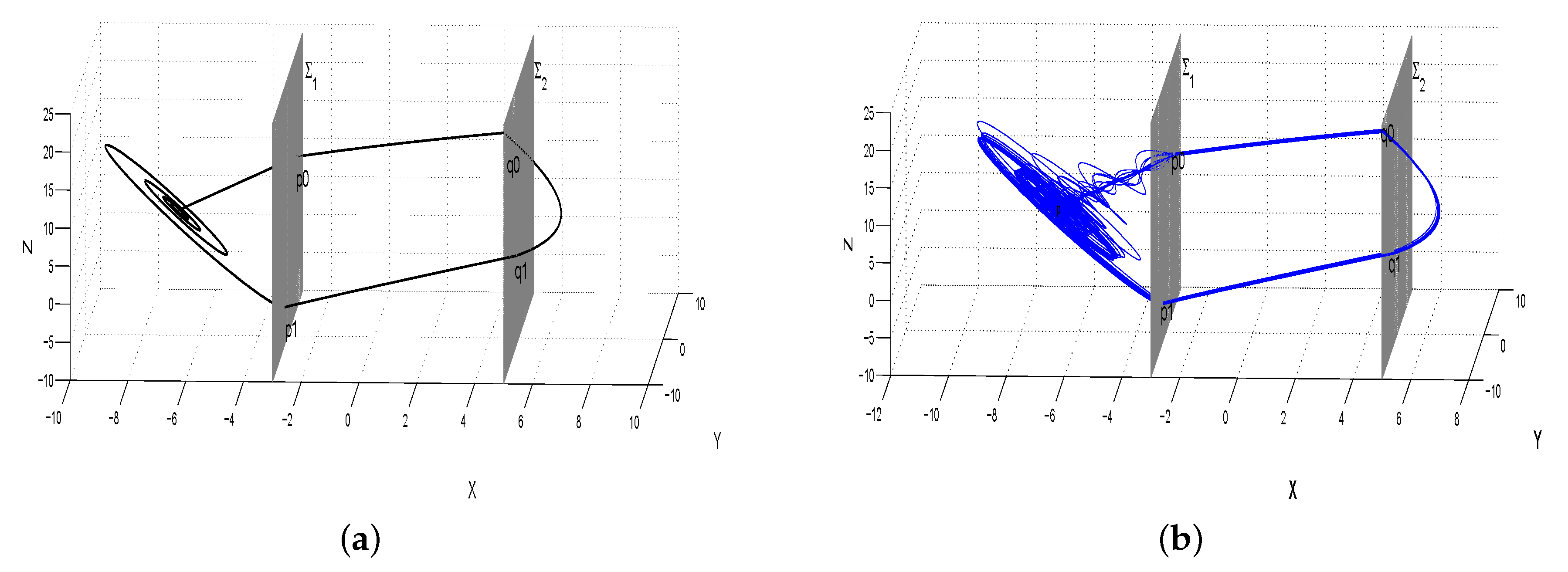
Example 1.

Consider the system

$$\dot{\mathbf{x}}=\left\{\begin{array}{c}\mathbf{A}\mathbf{x}+\mathbf{a},x\le -3,\hfill \\ \mathbf{B}\mathbf{x}+\mathbf{b},-3<x<5,\hfill \\ \mathbf{C}\mathbf{x}+\mathbf{c},x\ge 5,\hfill \end{array}\right.$$

(14)

where $\mathbf{A}=\mathbf{P}{\mathbf{J}}_{\mathbf{1}}{\mathbf{P}}^{-1}$, $\mathbf{B}=\mathbf{Q}{\mathbf{J}}_{\mathbf{2}}{\mathbf{Q}}^{-1}$ and $\mathbf{C}=\mathbf{R}{\mathbf{J}}_{\mathbf{3}}{\mathbf{R}}^{-1}$ with

$${\mathbf{J}}_{\mathbf{1}}=\left(\begin{array}{ccccc}1& & \hfill -8& & \hfill 0\\ 8& & \hfill 1& & \hfill 0\\ 0& & \hfill 0& & \hfill -1.1\end{array}\right),{\mathbf{J}}_{\mathbf{2}}=\left(\begin{array}{ccccc}-1& & \hfill 0& & \hfill 0\\ 0& & \hfill 0& & \hfill 0\\ 0& & \hfill 0& & \hfill 1\end{array}\right),{\mathbf{J}}_{\mathbf{3}}=\left(\begin{array}{ccccc}-1& & \hfill 0& & \hfill 0\\ 0& & \hfill 2& & \hfill 0\\ 0& & \hfill 0& & \hfill 3\end{array}\right),$$

$$\mathbf{P}=\left(\begin{array}{ccccc}-2& & \hfill -2& & \hfill 2\\ 4& & \hfill 2& & \hfill 1\\ 5& & \hfill 4& & \hfill 3\end{array}\right),\mathbf{Q}=\left(\begin{array}{ccccc}1& & \hfill 1& & \hfill 3\\ -3& & \hfill 1& & \hfill -1\\ 2& & \hfill 2& & \hfill 3\end{array}\right),\mathbf{R}=\left(\begin{array}{ccccc}-17/7& & \hfill 5/7& & \hfill 1\\ 2& & \hfill 1& & \hfill 1\\ -2& & \hfill 1& & \hfill -2\end{array}\right).$$

$$\mathbf{p}={(-7,4,4)}^{⊺}\in {\Sigma }_l,\mathbf{q}={(-5,16,0)}^{⊺},\mathbf{r}={(15,-10,7)}^{⊺},\mathbf{a}=-\mathbf{A}\mathbf{p},\mathbf{b}=-\mathbf{B}\mathbf{q},\mathbf{c}=-\mathbf{C}\mathbf{r}.$$

By trivial computation, we obtain that ${\mathbf{p}}_{\mathbf{0}}={(-3,6,10)}^{⊺}$, ${\mathbf{p}}_{\mathbf{1}}={(-3,-2,-5)}^{⊺}$, ${\mathbf{q}}_{\mathbf{1}}={(5,-2,2)}^{⊺}$ and ${\rho }_1=5,{\rho }_2=3,{\rho }_3=-2$, ${\sigma }_1=2,{\sigma }_2=-9,{\sigma }_3=3$, ${\tau }_1=4,{\tau }_2=1,$${\tau }_3=-1$.

Next, we verify the conditions in Theorem 1. Let $k_1=k_2=-1,T_{00}=-ln2,T_{10}=T_{11}=ln2$, then we have ${\mathbf{q}}_{\mathbf{0}}={(5,-10,23)}^{⊺}$. Moreover,

$$\alpha (d_1-x_p)+\beta (k_1{\xi }_{21}-k_2{\xi }_{11})=4>0,M{e}^{-\alpha T}\frac{\beta }{\sqrt{{\alpha }^2+{\beta }^2}}<4.$$

$$\frac{-{\sigma }_2{\lambda }_2({\lambda }_2-{\lambda }_1){\eta }_{21}}{{\sigma }_3{\lambda }_3({\lambda }_3-{\lambda }_1){\eta }_{31}}=0,$$

$${\sigma }_1{\lambda }_1{\eta }_{11}+{\sigma }_2{\lambda }_2{\eta }_{21}+{\sigma }_3{\lambda }_3{\eta }_{31}=7>0,$$

$${\sigma }_1{\lambda }_1{e}^{{\lambda }_1{T}_{11}}{\eta }_{11}+{\sigma }_2{\lambda }_2{e}^{{\lambda }_2{T}_{11}}{\eta }_{21}+{\sigma }_3{\lambda }_3{e}^{{\lambda }_3{T}_{11}}{\eta }_{31}=17>0,$$

$$\frac{-{\rho }_2{\lambda }_2({\lambda }_2-{\lambda }_1){\eta }_{21}}{{\rho }_3{\lambda }_3({\lambda }_3-{\lambda }_1){\eta }_{31}}=0,$$

$${\rho }_1{\lambda }_1{\eta }_{11}+{\rho }_2{\lambda }_2{\eta }_{21}+{\rho }_3{\lambda }_3{\eta }_{31}=-11<0,$$

$${\rho }_1{\lambda }_1{e}^{{\lambda }_1{T}_{00}}{\eta }_{11}+{\rho }_2{\lambda }_2{e}^{{\lambda }_2{T}_{00}}{\eta }_{21}+{\rho }_3{\lambda }_3{e}^{{\lambda }_3{T}_{00}}{\eta }_{31}=-13<0,$$

$${\tau }_1{\gamma }_1{\zeta }_{11}+{\tau }_2{\gamma }_2{\zeta }_{21}+{\tau }_3{\gamma }_3{\zeta }_{31}=57/7>0,$$

$${\tau }_1{\gamma }_1{e}^{{\gamma }_1{T}_{10}}{\zeta }_{11}+{\tau }_2{\gamma }_2{e}^{{\gamma }_2{T}_{10}}{\zeta }_{21}+{\tau }_3{\gamma }_3{e}^{{\gamma }_3{T}_{10}}{\zeta }_{31}=-94/7<0.$$

It can be seen that system (14) meets all the conditions in Theorem 1, so it has a homoclinic orbit to the equilibrium point $\mathbf{p}$.

Remark 2.

For piecewise affine systems, there are also some conclusions similar to Shil’nikov Theorem when Shil’nikov-like conditions are satisfied. Huan et al. [17] had given a rigorous proof by the topological horseshoe theorem [26,27] based on the ideas of Shil’nikov theorem.

Actually, because system (14) satisfies $\alpha +\lambda <0$, it has infinite numbers of chaotic invariant sets. Figure 1a,b show the system’s homoclinic orbit and a chaotic invariant set, respectively.

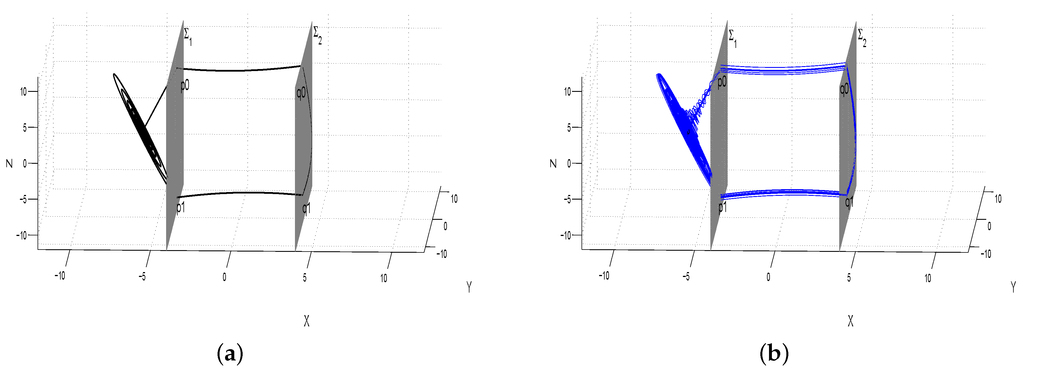
Example 2.

Consider the system

$$\dot{\mathbf{x}}=\left\{\begin{array}{c}\mathbf{A}\mathbf{x}+\mathbf{a},x\le -4,\hfill \\ \mathbf{B}\mathbf{x}+\mathbf{b},-4<x<4,\hfill \\ \mathbf{C}\mathbf{x}+\mathbf{c},x\ge 4,\hfill \end{array}\right.$$

(15)

where$\mathbf{A}=\mathbf{P}{\mathbf{J}}_{\mathbf{1}}{\mathbf{P}}^{-1}$,$\mathbf{B}=\mathbf{Q}{\mathbf{J}}_{\mathbf{2}}{\mathbf{Q}}^{-1}$and$\mathbf{C}=\mathbf{R}{\mathbf{J}}_{\mathbf{3}}{\mathbf{R}}^{-1}$with

$${\mathbf{J}}_{\mathbf{1}}=\left(\begin{array}{ccccc}1& & \hfill -20& & \hfill 0\\ 20& & \hfill 1& & \hfill 0\\ 0& & \hfill 0& & \hfill -1.1\end{array}\right),{\mathbf{J}}_{\mathbf{2}}=\left(\begin{array}{ccccc}-1& & \hfill 0& & \hfill 0\\ 0& & \hfill -1& & \hfill 0\\ 0& & \hfill 0& & \hfill 1\end{array}\right),{\mathbf{J}}_{\mathbf{3}}=\left(\begin{array}{ccccc}-1& & \hfill 0& & \hfill 0\\ 0& & \hfill 1& & \hfill 0\\ 0& & \hfill 0& & \hfill 2\end{array}\right),$$

$$\mathbf{P}=\left(\begin{array}{ccccc}1& & \hfill 1& & \hfill 2\\ -2& & \hfill 4& & \hfill 2\\ -4& & \hfill -6& & \hfill 8\end{array}\right),\mathbf{Q}=\left(\begin{array}{ccccc}2& & \hfill 2& & \hfill 4\\ -3& & \hfill 1& & \hfill -2\\ 3& & \hfill 1& & \hfill -2\end{array}\right),\mathbf{R}=\left(\begin{array}{ccccc}-2& & \hfill 1& & \hfill 1\\ 1& & \hfill -2& & \hfill -1\\ -4& & \hfill 2& & \hfill -4\end{array}\right).$$

$$\mathbf{p}={(-6,0,0)}^{⊺}\in {\Sigma }_l,\mathbf{q}={(0,0,0)}^{⊺},\mathbf{r}={(8,-3,-6)}^{⊺},\mathbf{a}=-\mathbf{A}\mathbf{p},\mathbf{b}=-\mathbf{B}\mathbf{q},\mathbf{c}=-\mathbf{C}\mathbf{r}.$$

By simple computation, we obtain that ${\mathbf{p}}_{\mathbf{0}}={(-4,2,8)}^{⊺}$, ${\mathbf{p}}_{\mathbf{1}}={(-4,2,-10)}^{⊺}$, ${\mathbf{q}}_{\mathbf{1}}={(4,-2,-8)}^{⊺}$ and ${\rho }_1=1,{\rho }_2=1,{\rho }_3=-2$, ${\sigma }_1=-2,{\sigma }_2=-2,{\sigma }_3=1$, ${\tau }_1=2,{\tau }_2=1,{\tau }_3=-1$.

Next, we verify the conditions in Theorem 1. Let $k_1=k_2=1,T_{00}=-ln2,T_{10}=T_{11}=ln2$, then we have ${\mathbf{q}}_{\mathbf{0}}={(4,-2,10)}^{⊺}$. Moreover,

$$\alpha (d_1-x_p)+\beta (k_1{\xi }_{21}-k_2{\xi }_{11})=2>0,M{e}^{-\alpha T}\frac{\beta }{\sqrt{{\alpha }^2+{\beta }^2}}<2.$$

$$\frac{-{\sigma }_2{\lambda }_2({\lambda }_2-{\lambda }_1){\eta }_{21}}{{\sigma }_3{\lambda }_3({\lambda }_3-{\lambda }_1){\eta }_{31}}=0,$$

$${\sigma }_1{\lambda }_1{\eta }_{11}+{\sigma }_2{\lambda }_2{\eta }_{21}+{\sigma }_3{\lambda }_3{\eta }_{31}=12>0,$$

$${\sigma }_1{\lambda }_1{e}^{{\lambda }_1{T}_{11}}{\eta }_{11}+{\sigma }_2{\lambda }_2{e}^{{\lambda }_2{T}_{11}}{\eta }_{21}+{\sigma }_3{\lambda }_3{e}^{{\lambda }_3{T}_{11}}{\eta }_{31}=12>0,$$

$$\frac{-{\rho }_2{\lambda }_2({\lambda }_2-{\lambda }_1){\eta }_{21}}{{\rho }_3{\lambda }_3({\lambda }_3-{\lambda }_1){\eta }_{31}}=0,$$

$${\rho }_1{\lambda }_1{\eta }_{11}+{\rho }_2{\lambda }_2{\eta }_{21}+{\rho }_3{\lambda }_3{\eta }_{31}=-12<0,$$

$${\rho }_1{\lambda }_1{e}^{{\lambda }_1{T}_{00}}{\eta }_{11}+{\rho }_2{\lambda }_2{e}^{{\lambda }_2{T}_{00}}{\eta }_{21}+{\rho }_3{\lambda }_3{e}^{{\lambda }_3{T}_{00}}{\eta }_{31}=-12<0,$$

$${\tau }_1{\gamma }_1{\zeta }_{11}+{\tau }_2{\gamma }_2{\zeta }_{21}+{\tau }_3{\gamma }_3{\zeta }_{31}=3>0,$$

$${\tau }_1{\gamma }_1{e}^{{\gamma }_1{T}_{10}}{\zeta }_{11}+{\tau }_2{\gamma }_2{e}^{{\gamma }_2{T}_{10}}{\zeta }_{21}+{\tau }_3{\gamma }_3{e}^{{\gamma }_3{T}_{10}}{\zeta }_{31}=-4<0.$$

Obviously, system (15) also satisfies all the conditions in Theorem 1, thus it has a homoclinic orbit to the equilibrium point $\mathbf{p}$. Similarly, system (15) meets $\alpha +\lambda <0$, implying that it has an infinite number of chaotic invariant sets. Figure 2a,b show the system’s homoclinic orbit and a chaotic invariant set, respectively.

3. The Existence of Two Homoclinic Orbits

In the sequel, we suppose that the homoclinic equilibrium point lies between the switching planes ${\Sigma }_1$ and ${\Sigma }_2$. We consider the three-dimensional piecewise affine systems as follows:

$$\dot{\mathbf{x}}=\left\{\begin{array}{c}\mathbf{B}\mathbf{x}+\mathbf{b},x\le d_1,\hfill \\ \mathbf{A}\mathbf{x}+\mathbf{a},d_1<x<d_2,\hfill \\ \mathbf{C}\mathbf{x}+\mathbf{c},x\ge d_2,\hfill \end{array}\right.$$

(16)

which have the same elements as system (1).

Now, we assume that the equilibrium point $\mathbf{p}$ corresponding the middle system of (16) lies between the switching planes ${\Sigma }_1$ and ${\Sigma }_2$ (i.e., $d_1<x_p<d_2$) and $E^s\left(\mathbf{p}\right)\bigcap {\Sigma }_1\ne ⌀$, $E^u\left(\mathbf{p}\right)\bigcap {\Sigma }_1\ne ⌀$. Then we have $E^s\left(\mathbf{p}\right)\bigcap {\Sigma }_2\ne ⌀$ and $E^u\left(\mathbf{p}\right)\bigcap {\Sigma }_2\ne ⌀$ since plane ${\Sigma }_2$ is Parallel to ${\Sigma }_1$. Denote ${\mathbf{q}}_{\mathbf{0}}=E^s\left(\mathbf{p}\right)\cap {\Sigma }_2$ and $l_2=E^u\left(\mathbf{p}\right)\cap {\Sigma }_2$, then we have

$${\mathbf{q}}_{\mathbf{0}}={(d_2,y_p+\frac{d_2-x_p}{{\xi }_{31}}{\xi }_{32},z_p+\frac{d_2-x_p}{{\xi }_{31}}{\xi }_{33})}^{⊺},$$

$$l_2=\{\mathbf{x}=\mathbf{p}+k_1^{\prime }{\xi }_{\mathbf{1}}+k_2^{\prime }{\xi }_{\mathbf{2}}\mid x_p+k_1^{\prime }{\xi }_{11}+k_2^{\prime }{\xi }_{21}=d_2,k_1^{\prime },k_2^{\prime }\in \mathbf{R}\}.$$

Next, we give a sufficient condition for the existence of two homoclinic orbits of system (16).

Theorem 2.

If the following conditions hold for system (16):

(i) There exist real numbers $k_1,k_2$ such that ${\mathbf{p}}_{\mathbf{1}}\in l_1$ and

$$\alpha (d_1-x_p)+\beta (k_1{\xi }_{21}-k_2{\xi }_{11})<0,$$

$$M_1{e}^{-\alpha T_1}\frac{\beta }{\sqrt{{\alpha }^2+{\beta }^2}}<d_2-x_p,M_1{e}^{-\alpha T_2}\frac{-\beta }{\sqrt{{\alpha }^2+{\beta }^2}}>d_1-x_p,$$

where

$$M_1=\sqrt{{(d_1-x_p)}^2+{(k_1{\xi }_{21}-k_2{\xi }_{11})}^2},$$

$$T_1=\frac{arctan\left(\frac{\beta }{\alpha }\right)-arcsin\left(\frac{x_p-d_1}{M_1}\right)}{\beta },T_2=\frac{\pi +arctan\left(\frac{\beta }{\alpha }\right)-arcsin\left(\frac{x_p-d_1}{M_1}\right)}{\beta };$$

(ii) There exists a constant $T_3>0$ such that

$${\mathbf{p}}_{\mathbf{0}}=\mathbf{q}+\left({\eta }_1{\eta }_2{\eta }_3\right){\left({\sigma }_1{e}^{{\lambda }_1{T}_3}{\sigma }_2{e}^{{\lambda }_2{T}_3}{\sigma }_3{e}^{{\lambda }_3{T}_3}\right)}^{⊺},x_q+{\sigma }_1{e}^{{\lambda }_1{T}_3}{\eta }_{11}+{\sigma }_2{e}^{{\lambda }_2{T}_3}{\eta }_{21}+{\sigma }_3{e}^{{\lambda }_3{T}_3}{\eta }_{31}=d_1,$$

$${\sigma }_1{\lambda }_1{\eta }_{11}+{\sigma }_2{\lambda }_2{\eta }_{21}+{\sigma }_3{\lambda }_3{\eta }_{31}<0,{\sigma }_1{\lambda }_1{e}^{{\lambda }_1{T}_3}{\eta }_{11}+{\sigma }_2{\lambda }_2{e}^{{\lambda }_2{T}_3}{\eta }_{21}+{\sigma }_3{\lambda }_3{e}^{{\lambda }_3{T}_3}{\eta }_{31}>0.$$

Here, ${({\sigma }_1,{\sigma }_2,{\sigma }_3)}^{⊺}$ is the coordinate of ${\mathbf{p}}_{\mathbf{1}}$ under the coordinate system $\{\mathbf{q};{\eta }_1,{\eta }_2,{\eta }_3\}$.

(iii) There exist real numbers $k_1^{\prime },k_2^{\prime }$ such that ${\mathbf{q}}_{\mathbf{1}}\in l_2$ and

$$\alpha (d_2-x_p)+\beta (k_1^{\prime }{\xi }_{21}-k_2^{\prime }{\xi }_{11})>0,$$

$$M_2{e}^{-\alpha T_1^{\prime }}\frac{-\beta }{\sqrt{{\alpha }^2+{\beta }^2}}>d_1-x_p,M_2{e}^{-\alpha T_2^{\prime }}\frac{\beta }{\sqrt{{\alpha }^2+{\beta }^2}}<d_2-x_p,$$

where

$$M_2=\sqrt{{(d_2-x_p)}^2+{(k_1^{\prime }{\xi }_{21}-k_2^{\prime }{\xi }_{11})}^2},$$

$$T_1^{\prime }=\frac{arctan(\frac{\beta }{\alpha })+arcsin(\frac{d_2-x_p}{M_2})}{\beta },T_2^{\prime }=\frac{\pi +arctan(\frac{\beta }{\alpha })+arcsin(\frac{d_2-x_p}{M_2})}{\beta };$$

(iv) There exists a constant $T_4>0$ such that

$${\mathbf{q}}_{\mathbf{0}}=\mathbf{r}+\left({\zeta }_{\mathbf{1}}{\zeta }_{\mathbf{2}}{\zeta }_{\mathbf{3}}\right){\left({\tau }_1{e}^{{\gamma }_1{T}_4}{\tau }_2{e}^{{\gamma }_2{T}_4}{\tau }_3{e}^{{\gamma }_3{T}_4}\right)}^{⊺},x_r+{\tau }_1{e}^{{\gamma }_1{T}_4}{\zeta }_{11}+{\tau }_2{e}^{{\gamma }_2{T}_4}{\zeta }_{21}+{\tau }_3{e}^{{\gamma }_3{T}_4}{\zeta }_{31}=d_2,$$

$${\tau }_1{\gamma }_1{\zeta }_{11}+{\tau }_2{\gamma }_2{\zeta }_{21}+{\tau }_3{\gamma }_3{\zeta }_{31}>0,{\tau }_1{\gamma }_1{e}^{{\gamma }_1{T}_4}{\zeta }_{11}+{\tau }_2{\gamma }_2{e}^{{\gamma }_2{T}_4}{\zeta }_{21}+{\tau }_3{\gamma }_3{e}^{{\gamma }_3{T}_4}{\zeta }_{31}<0.$$

Here, ${({\tau }_1,{\tau }_2,{\tau }_3)}^{⊺}$ is the coordinate of ${\mathbf{q}}_{\mathbf{1}}$ under the coordinate system $\{\mathbf{r};{\zeta }_1,{\zeta }_2,{\zeta }_3\}$.

Then system (16) has two orbits ${\Gamma }_l$ and ${\Gamma }_r$, which are both homoclinic to the equilibrium point $\mathbf{p}$. Moreover, ${\Gamma }_l$ crosses the switching plane ${\Sigma }_1$ transversally at ${\mathbf{p}}_{\mathbf{0}}$ and ${\mathbf{p}}_{\mathbf{1}}$, meanwhile ${\Gamma }_r$ crosses the switching plane ${\Sigma }_2$ transversally at ${\mathbf{q}}_{\mathbf{0}}$ and ${\mathbf{q}}_{\mathbf{1}}$.

Proof. 

Because conditions (iii)–(iv) are similar to conditions (i)–(ii), we only prove the first two here. It is equivalent to proving that there is a homoclinic orbit ${\Gamma }_l$ to the equilibrium point $\mathbf{p}$ with transversal crossing ${\Sigma }_1$ at ${\mathbf{p}}_{\mathbf{0}}$ and ${\mathbf{p}}_{\mathbf{1}}$. That is, the following conditions hold:

(1)

${\mathbf{p}}_{\mathbf{1}}\in l_1;$

(2)

The positive orbit of ${\mathbf{p}}_{\mathbf{0}}$ satisfies

$$O_{+}\left({\mathbf{p}}_{\mathbf{0}}\right)=\{{\varphi }_1(t,{\mathbf{p}}_{\mathbf{0}})\mid t>0\}\subset {\Sigma }_m;$$

(3)

The negative orbit of ${\mathbf{p}}_{\mathbf{1}}$ satisfies

$$O_{-}\left({\mathbf{p}}_{\mathbf{1}}\right)=\{{\varphi }_1(t,{\mathbf{p}}_{\mathbf{1}})\mid t<0\}\subset {\Sigma }_m;$$

(4)

There exists a constant $T_3>0$, such that

$$\{{\varphi }_2(t,{\mathbf{p}}_{\mathbf{1}})\mid t\in (0,T_3)\}\subset {\Sigma }_{l}and{\varphi }_2(T_3,{\mathbf{p}}_{\mathbf{1}})={\mathbf{p}}_{\mathbf{0}}\in {\Sigma }_1;$$

(5)

$${\mathbf{n}}^{⊺}(\mathbf{A}{\mathbf{p}}_{\mathbf{0}}+\mathbf{a}){\mathbf{n}}^{⊺}(\mathbf{B}{\mathbf{p}}_{\mathbf{0}}+\mathbf{b})>0,{\mathbf{n}}^{⊺}(\mathbf{A}{\mathbf{p}}_{\mathbf{1}}+\mathbf{a}){\mathbf{n}}^{⊺}(\mathbf{B}{\mathbf{p}}_{\mathbf{1}}+\mathbf{b})>0.$$

Condition (5) ensures that the homoclinic orbit ${\Gamma }_l$ crosses ${\Sigma }_1$ transversally at ${\mathbf{p}}_{\mathbf{0}}$ and ${\mathbf{p}}_{\mathbf{1}}$.

Conditions $\left(1\right)$ and $\left(2\right)$ clearly hold.

For condition $\left(3\right)$, we still denote $f_1\left(t\right)={\mathbf{n}}^{⊺}({\varphi }_1(-t,{\mathbf{p}}_{\mathbf{1}})-\mathbf{p})$, then

$$f_1\left(t\right)=M_1{e}^{-\alpha t}sin(-\beta t+{\theta }_1),$$

where

$$M_1=\sqrt{{(d_1-x_p)}^2+{(k_1{\xi }_{21}-k_2{\xi }_{11})}^2},sin{\theta }_1=\frac{d_1-x_p}{M},cos{\theta }_1=\frac{k_1{\xi }_{21}-k_2{\xi }_{11}}{M}.$$

Therefore, $O_{-}\left({\mathbf{p}}_{\mathbf{1}}\right)=\{{\varphi }_1(t,{\mathbf{p}}_{\mathbf{1}})\mid t<0\}\subset {\Sigma }_m$ if and only if $d_1-x_p<f_1\left(t\right)<d_2-x_p$ holds for all $t>0$. With a simple calculation, we obtain

$$f_1\left(0\right)=d_1-x_p,f_1^{\prime }\left(0\right)=-\alpha (d_1-x_p)-\beta (k_1{\xi }_{21}-k_2{\xi }_{11}).$$

Similar to the previous analysis, we request $f_1^{\prime }\left(0\right)>0$,, i.e.,

$$\alpha (d_1-x_p)+\beta (k_1{\xi }_{21}-k_2{\xi }_{11})<0.$$

On the other hand, we need that $d_1-x_p<f_1\left(T_1\right),f_1\left(T_2\right)<d_2-x_p$ for the local extreme points $T_1,T_2\in (0,\frac{2\pi }{\beta })$. Here,

$$T_1=\frac{arctan(\frac{\beta }{\alpha })-arcsin(\frac{x_p-d_1}{M_1})}{\beta },T_2=\frac{\pi +arctan(\frac{\beta }{\alpha })-arcsin(\frac{x_p-d_1}{M_1})}{\beta },$$

are the local maximum and minimum points in $(0,\frac{2\pi }{\beta })$, respectively. Thus, we can get $O_{-}\left({\mathbf{p}}_{\mathbf{1}}\right)=\{{\varphi }_1(t,{\mathbf{p}}_1)\mid t<0\}\subset {\Sigma }_m$ by condition (i).

Since the proofs of condition $\left(4\right)$ and $\left(5\right)$ are similar to the ones in Theorem 1, the details are omitted here. The proof is then completed. □

Next, we give two examples to illustrate the effectiveness of the conclusion in Theorem 2.

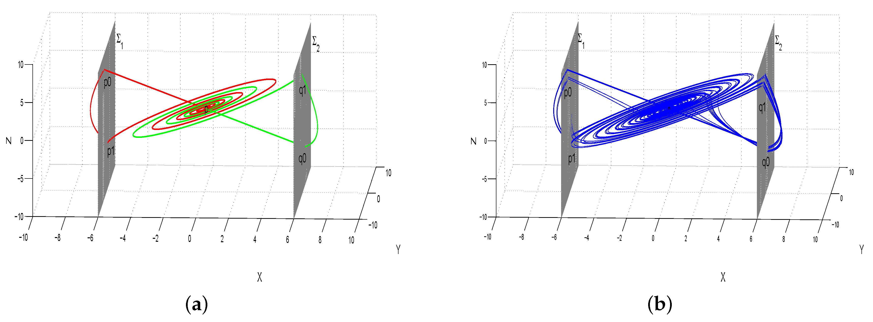
Example 3.

Consider the system

$$\dot{\mathbf{x}}=\left\{\begin{array}{c}\mathbf{B}\mathbf{x}+\mathbf{b},x\le -6,\hfill \\ \mathbf{A}\mathbf{x}+\mathbf{a},-6<x<6,\hfill \\ \mathbf{C}\mathbf{x}+\mathbf{c},x\ge 6,\hfill \end{array}\right.$$

(17)

where $\mathbf{A}=\mathbf{P}{\mathbf{J}}_{\mathbf{1}}{\mathbf{P}}^{-1}$, $\mathbf{B}=\mathbf{Q}{\mathbf{J}}_{\mathbf{2}}{\mathbf{Q}}^{-1}$ and $\mathbf{C}=\mathbf{R}{\mathbf{J}}_{\mathbf{3}}{\mathbf{R}}^{-1}$ with

$${\mathbf{J}}_{\mathbf{1}}=\left(\begin{array}{ccccc}1& & \hfill -10& & \hfill 0\\ 10& & \hfill 1& & \hfill 0\\ 0& & \hfill 0& & \hfill -20\end{array}\right),{\mathbf{J}}_{\mathbf{2}}=\left(\begin{array}{ccccc}-1& & \hfill 0& & \hfill 0\\ 0& & \hfill 1& & \hfill 0\\ 0& & \hfill 0& & \hfill 2\end{array}\right),{\mathbf{J}}_{\mathbf{3}}=\left(\begin{array}{ccccc}-2& & \hfill 0& & \hfill 0\\ 0& & \hfill -1& & \hfill 0\\ 0& & \hfill 0& & \hfill 1\end{array}\right),$$

$$\mathbf{P}=\left(\begin{array}{ccccc}3& & \hfill 3& & \hfill 2\\ -2& & \hfill 1& & \hfill 1\\ 2& & \hfill 3& & \hfill -2\end{array}\right),\mathbf{Q}=\left(\begin{array}{ccccc}2& & \hfill 1& & \hfill 1\\ 2& & \hfill 3& & \hfill -1\\ -2& & \hfill -2& & \hfill 3\end{array}\right),\mathbf{R}=\left(\begin{array}{ccccc}3/2& & \hfill 3/2& & \hfill -3\\ 1& & \hfill 2& & \hfill 3\\ -5& & \hfill -3& & \hfill 1\end{array}\right).$$

$$\mathbf{p}={(0,0,1)}^{⊺}\in {\Sigma }_m,\mathbf{q}={(-16,-9,3)}^{⊺},\mathbf{r}={(12,-4,-9)}^{⊺},\mathbf{a}=-\mathbf{A}\mathbf{p},\mathbf{b}=-\mathbf{B}\mathbf{q},\mathbf{c}=-\mathbf{C}\mathbf{r}.$$

Let $k_1=k_2=-1,k_1^{\prime }=k_2^{\prime }=1,T_3=T_4=ln2$, we can obtain that ${\mathbf{p}}_{\mathbf{0}}={(-6,-3,7)}^{⊺}$, ${\mathbf{p}}_{\mathbf{1}}={(-6,1,-4)}^{⊺}$, ${\mathbf{q}}_{\mathbf{0}}={(6,3,-5)}^{⊺}$, ${\mathbf{q}}_{\mathbf{1}}={(6,-1,6)}^{⊺}$ and ${\sigma }_1=4,{\sigma }_2=1,{\sigma }_3=1$, ${\tau }_1=-4,{\tau }_2=2,{\tau }_3=1$.

Next, we verify the conditions in Theorem 2.

$$\alpha (d_1-x_p)+\beta (k_1{\xi }_{21}-k_2{\xi }_{11})=-6<0,$$

$$M_1{e}^{-\alpha T_1}\frac{\beta }{\sqrt{{\alpha }^2+{\beta }^2}}<6=d_2-x_p,M_1{e}^{-\alpha T_2}\frac{-\beta }{\sqrt{{\alpha }^2+{\beta }^2}}>-6=d_1-x_p.$$

$${\sigma }_1{\lambda }_1{\eta }_{11}+{\sigma }_2{\lambda }_2{\eta }_{21}+{\sigma }_3{\lambda }_3{\eta }_{31}=-5<0,$$

$${\sigma }_1{\lambda }_1{e}^{{\lambda }_1{T}_3}{\eta }_{11}+{\sigma }_2{\lambda }_2{e}^{{\lambda }_2{T}_3}{\eta }_{21}+{\sigma }_3{\lambda }_3{e}^{{\lambda }_3{T}_3}{\eta }_{31}=2>0,$$

$$\alpha (d_2-x_p)+\beta (k_1^{\prime }{\xi }_{21}-k_2^{\prime }{\xi }_{11})=6>0,$$

$$M_2{e}^{-\alpha T_1^{\prime }}\frac{-\beta }{\sqrt{{\alpha }^2+{\beta }^2}}>-6=d_1-x_p,M_2{e}^{-\alpha T_2^{\prime }}\frac{\beta }{\sqrt{{\alpha }^2+{\beta }^2}}<6=d_2-x_p,$$

$${\tau }_1{\gamma }_1{\zeta }_{11}+{\tau }_2{\gamma }_2{\zeta }_{21}+{\tau }_3{\gamma }_3{\zeta }_{31}=6>0,$$

$${\tau }_1{\gamma }_1{e}^{{\gamma }_1{T}_4}{\zeta }_{11}+{\tau }_2{\gamma }_2{e}^{{\gamma }_2{T}_4}{\zeta }_{21}+{\tau }_3{\gamma }_3{e}^{{\gamma }_3{T}_4}{\zeta }_{31}=-9/2<0.$$

As a result, system (17) meets all the conditions in Theorem 2, it has two homoclinic orbits to the equilibrium point $\mathbf{p}$. Simultaneously, it also satisfies the Shil’nikov conditions from $\alpha +\lambda <0$, implying that it has infinite numbers of chaotic invariant sets. Figure 3a,b show the system’s two homoclinic orbits and a chaotic invariant set, respectively.

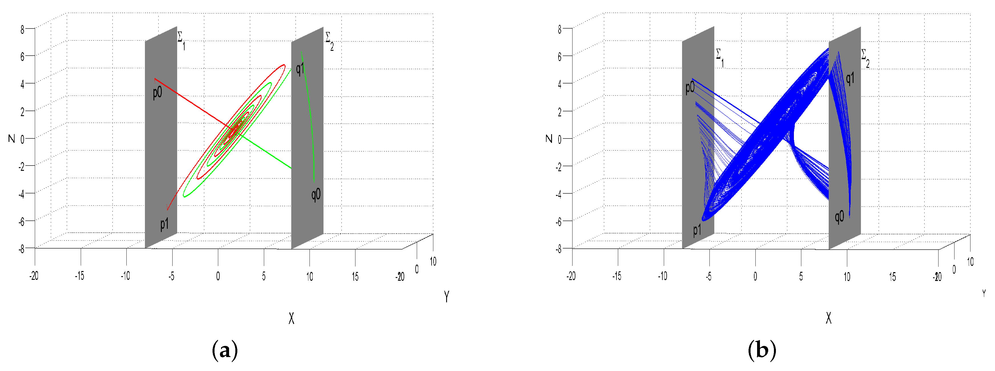
Example 4.

Consider the system

$$\dot{\mathbf{x}}=\left\{\begin{array}{c}\mathbf{B}\mathbf{x}+\mathbf{b},x\le -8,\hfill \\ \mathbf{A}\mathbf{x}+\mathbf{a},-8<x<8,\hfill \\ \mathbf{C}\mathbf{x}+\mathbf{c},x\ge 8,\hfill \end{array}\right.$$

(18)

where $\mathbf{A}=\mathbf{P}{\mathbf{J}}_{\mathbf{1}}{\mathbf{P}}^{-1}$, $\mathbf{B}=\mathbf{Q}{\mathbf{J}}_{\mathbf{2}}{\mathbf{Q}}^{-1}$ and $\mathbf{C}=\mathbf{R}{\mathbf{J}}_{\mathbf{3}}{\mathbf{R}}^{-1}$ with

$${\mathbf{J}}_{\mathbf{1}}=\left(\begin{array}{ccccc}1& & \hfill -10& & \hfill 0\\ 10& & \hfill 1& & \hfill 0\\ 0& & \hfill 0& & \hfill -20\end{array}\right),{\mathbf{J}}_{\mathbf{2}}=\left(\begin{array}{ccccc}-1& & \hfill 0& & \hfill 0\\ 0& & \hfill 0& & \hfill 0\\ 0& & \hfill 0& & \hfill 1\end{array}\right),{\mathbf{J}}_{\mathbf{3}}=\left(\begin{array}{ccccc}-1& & \hfill 0& & \hfill 0\\ 0& & \hfill -1& & \hfill 0\\ 0& & \hfill 0& & \hfill 1\end{array}\right),$$

$$\mathbf{P}=\left(\begin{array}{ccccc}2& & \hfill 2& & \hfill 4\\ -3& & \hfill 1& & \hfill 2\\ 1& & \hfill 2& & \hfill -2\end{array}\right),\mathbf{Q}=\left(\begin{array}{ccccc}2& & \hfill 1& & \hfill 1\\ 2& & \hfill 3& & \hfill -1\\ -2& & \hfill -2& & \hfill 3\end{array}\right),\mathbf{R}=\left(\begin{array}{ccccc}-1& & \hfill -1& & \hfill -2\\ -2& & \hfill -4& & \hfill 2\\ 4& & \hfill 3& & \hfill -3\end{array}\right).$$

$$\mathbf{p}={(0,0,0)}^{⊺}\in {\Sigma }_m,\mathbf{q}={(-12,1,0)}^{⊺},\mathbf{r}={(14,6,-5)}^{⊺},\mathbf{a}=-\mathbf{A}\mathbf{p},\mathbf{b}=-\mathbf{B}\mathbf{q},\mathbf{c}=-\mathbf{C}\mathbf{r}.$$

Let $k_1=k_2=-2,k_1^{\prime }=k_2^{\prime }=2,T_3=T_4=ln2$, we can obtain that ${\mathbf{p}}_{\mathbf{0}}={(-8,-4,4)}^{⊺}$, ${\mathbf{p}}_{\mathbf{1}}={(-8,4,-6)}^{⊺}$, ${\mathbf{q}}_{\mathbf{0}}={(8,4,-4)}^{⊺}$, ${\mathbf{q}}_{\mathbf{1}}={(8,-4,6)}^{⊺}$ and ${\sigma }_1=2,{\sigma }_2=1,{\sigma }_3=1$, ${\tau }_1=2,{\tau }_2=2,{\tau }_3=1$.

Next, we verify the conditions in Theorem 2.

$$\alpha (d_1-x_p)+\beta (k_1{\xi }_{21}-k_2{\xi }_{11})=-8<0,$$

$$M_1{e}^{-\alpha T_1}\frac{\beta }{\sqrt{{\alpha }^2+{\beta }^2}}<8=d_2-x_p,M_1{e}^{-\alpha T_2}\frac{-\beta }{\sqrt{{\alpha }^2+{\beta }^2}}>-8=d_1-x_p.$$

$${\sigma }_1{\lambda }_1{\eta }_{11}+{\sigma }_2{\lambda }_2{\eta }_{21}+{\sigma }_3{\lambda }_3{\eta }_{31}=-1<0,$$

$${\sigma }_1{\lambda }_1{e}^{{\lambda }_1{T}_3}{\eta }_{11}+{\sigma }_2{\lambda }_2{e}^{{\lambda }_2{T}_3}{\eta }_{21}+{\sigma }_3{\lambda }_3{e}^{{\lambda }_3{T}_3}{\eta }_{31}=1>0,$$

$$\alpha (d_2-x_p)+\beta (k_1^{\prime }{\xi }_{21}-k_2^{\prime }{\xi }_{11})=8>0,$$

$$M_2{e}^{-\alpha T_1^{\prime }}\frac{-\beta }{\sqrt{{\alpha }^2+{\beta }^2}}>-8=d_1-x_p,M_2{e}^{-\alpha T_2^{\prime }}\frac{\beta }{\sqrt{{\alpha }^2+{\beta }^2}}<8=d_2-x_p,$$

$${\tau }_1{\gamma }_1{\zeta }_{11}+{\tau }_2{\gamma }_2{\zeta }_{21}+{\tau }_3{\gamma }_3{\zeta }_{31}=2>0,$$

$${\tau }_1{\gamma }_1{e}^{{\gamma }_1{T}_4}{\zeta }_{11}+{\tau }_2{\gamma }_2{e}^{{\gamma }_2{T}_4}{\zeta }_{21}+{\tau }_3{\gamma }_3{e}^{{\gamma }_3{T}_4}{\zeta }_{31}=-2<0.$$

System (18) meets all the conditions in Theorem 2, thus it has two homoclinic orbits to the equilibrium point $\mathbf{p}$. It also satisfies the Shil’nikov conditions from $\alpha +\lambda <0$, so it has infinite numbers of chaotic invariant sets. Figure 4a,b show the system’s two homoclinic orbits and a chaotic invariant set, respectively.

4. Conclusions

We present an analytic method for determining the existence of homoclinic orbits in two classes of three-dimensional piecewise affine systems with two switching planes. In particular, several sufficient conditions for the existence of single and two homoclinic orbits are presented. In fact, when the equilibrium point $\mathbf{p}$ lies in ${\Sigma }_m$, we can still obtain some sufficient conditions for the existence of one homoclinic orbit in system (16). However, in order to avoid confusion between construction and notation, we do not consider this case here.

Additionally, for piecewise affine systems with more switching planes, our promoted method can be used to generate more homoclinic orbits or heteroclinic cycles. Furthermore, multi-scroll chaos generation and complex chaos circuits are possible. It can be also similarly used to investigate the existence of periodic orbits, homoclinic orbits, or heteroclinic cycles in some three-dimensional piecewise-linear discontinuous systems.

References

1. Chertovskih, R.; Gama, S.; Podvigina, O.; Zheligovsky, V. Dependence of magnetic field generation by thermal convection on the rotation rate: A case study. Phys. Nonlinear Phenom. 2010, 239, 1188–1209. [Google Scholar] [CrossRef] [Green Version]
2. Li, J.; Tomsovic, S. Homoclinic orbit expansion of arbitrary trajectories in chaotic systems: Classical action function and its memory. arXiv 2020, arXiv:2009.12224. [Google Scholar]
3. Chua, L.; Komuro, M.; Matsumoto, T. The double scroll family. IEEE Trans. Circuits Syst. 1986, 33, 1072–1118. [Google Scholar] [CrossRef] [Green Version]
4. Brown, R. Generalizations of the Chua equations. IEEE Tran. Circuits Syst.-I 1993, 40, 878–884. [Google Scholar] [CrossRef]
5. Shil’nikov, L.P. A case of the existence of a countable number of periodic motions. Sov. Math. Dokl. 1965, 6, 163–166. [Google Scholar]
6. Tresser, C. About some theorems by L.P. Shil’nikov. Inst. H. Poincaré Phys. Thoré 1984, 4, 441–461. [Google Scholar]
7. Shil’nikov, L.P.; Shil’nikov, A.L.; Turaev, D.V.; Chua, L.O. Methods of Qualitative Theory in Nonlinear Dynamics; World Scientific: Sigapore, 2001. [Google Scholar]
8. Wiggins, S. Introduction to Applied Nonlinear Dynamical Systems and Chaos, 2nd ed.; Springer: New York, NY, USA, 2003. [Google Scholar]
9. Deng, B. Constructing homoclinic orbits and chaotic attractors. Int. J. Bifurc. Chaos 1994, 4, 823–841. [Google Scholar] [CrossRef]
10. Cao, Y.; Chung, K.W.; Xu, J. A novel construction of homoclinic and heteroclinic orbits in nonlinear oscillators by a perturbation-incremental method. Nonlinear Dyn. 2011, 64, 221–236. [Google Scholar] [CrossRef]
11. Bao, J.; Yang, Q. A new method to fifind homoclinic and heteroclinic orbits. Appl. Math. Comput. 2011, 217, 6526–6540. [Google Scholar]
12. Choudhury, S.R.; Gambino, G. Convergent analytic solutions for homoclinic orbits in reversible and non-reversible systems. Nonlinear Dyn. 2013, 73, 1769–1782. [Google Scholar] [CrossRef] [Green Version]
13. Bai, F.; Spence, A.; Stuart, A.M. The numerical computation of heteroclinic connections in systems of gradient partial differential equations. SIAM J. Appl. Math. 1993, 53, 743–769. [Google Scholar] [CrossRef]
14. Freire, E.; Pizarro, L.; Rodríguez-Luis, A.J. Numerical continuation of homoclinic orbits to non-hyperbolic equilibria in planar systems. Nonlinear Dyn. 2000, 23, 353–375. [Google Scholar] [CrossRef]
15. Leonov, G. Fishing principle for homoclinic and heteroclinic trajectories. Nonlinear Dyn. 2014, 78, 2751–2758. [Google Scholar] [CrossRef]
16. Llibre, J.; Ponce, E.; Teruel, A.E. Horseshoes near homoclinic orbits for piecewise linear differential systems in R3. Internat. J. Bifur. Chaos 2007, 17, 1171–1184. [Google Scholar] [CrossRef]
17. Huan, S.; Li, Q.; Yang, X.S. Chaos in three-dimensional hybrid systems and design of chaos generators. Nonlinear Dyn. 2012, 69, 1915–1927. [Google Scholar] [CrossRef]
18. Wu, T.; Yang, X.S. A new class of 3-dimensional piecewise affine systems with homoclinic orbits. Discrete Contin. Dyn. Syst. 2016, 36, 5119–5129. [Google Scholar] [CrossRef]
19. Chen, Y.; Wu, T.; Yang, X.S. On the existence of homoclinic orbits in 3-dimensional piecewise affine systems. Comput. Appl. Math. 2018, 37, 6022–6033. [Google Scholar] [CrossRef]
20. Wu, T.; Yang, X.S. Construction of a Class of Four-Dimensional Piecewise Affine Systems with Homoclinic Orbits. Int. J. Bifur. Chaos 2016, 26, 1650099. [Google Scholar] [CrossRef]
21. Yang, X.S.; Li, Q. On entropy of Chua’s circuits. Internat. J. Bifur. Chaos 2005, 15, 1823–1828. [Google Scholar] [CrossRef]
22. Yalcin M., E.; Suykens, J.; Vandewalle, J. True random bit generation from a double-scroll attractor. IEEE Trans. Circuits Syst. I Fundam. Theory Appl. 2004, 51, 1395–1404. [Google Scholar] [CrossRef]
23. Yu, S.; Lü, J.; Chen, G.; Yu, X. Design of grid multi-wing butterfly chaotic attractors from piecewise Lü system based on switching control and heteroclinic orbit. In Proceedings of the IEEE International Symposium of Circuits Systems, Rio de Janeiro, Brazil, 15–18 May 2011. [Google Scholar]
24. Lü, J.; Yu, S.; Leung, H.; Chen, G. Experimental verification of multidirectional multiscroll chaotic attractors. IEEE Trans. Circuits Syst. Regul. Pap. 2006, 53, 149–165. [Google Scholar]
25. Lü, J.; Chen, G. Generating Multiscroll Chaotic Attractors: Theories, Methods and applications. Int. J. Bifur. Chaos 2006, 16, 775–858. [Google Scholar] [CrossRef]
26. Yang, X.S.; Tang, Y. Horseshoes in piecewise continuous maps. Chaos Solitons Fract. 2004, 19, 841–845. [Google Scholar] [CrossRef]
27. Yang, X.S. Topological horseshoes and computer assisted verification of chaotic dynamics. Int. J. Bifur. Chaos 2009, 19, 1127–1145. [Google Scholar] [CrossRef]
Figure 1. (a) The homoclinic orbit of Example 1 connects the equilibrium point p to itself which crosses the switching planes Σ 1 and Σ 2 transversally at p 0 , p 1 , q 0 , q 1 , respectively. (b) A chaotic invariant set of Example 1 near the homoclinic orbit.
Mathematics 09 03285 g001
Figure 2. (a) The homoclinic orbit of Example 2 connects the equilibrium point p to itself which crosses the switching planes Σ 1 and Σ 2 transversally at p 0 , p 1 , q 0 , q 1 , respectively; (b) A chaotic invariant set of Example 2 near the homoclinic orbit.
Mathematics 09 03285 g002
Figure 3. (a) The two homoclinic orbits of Example 3 are represented by red and green lines, respectively, which are both homoclinic to the saddle-focus equilibrium point p ; (b) A chaotic invariant set of Example 3 near the two homocliic orbits.
Mathematics 09 03285 g003
Figure 4. (a) The two homoclinic orbits of Example 4 e.g., adapted from Plew [15], with permission from American Society of Civil Engineers, 2011. are represented by red and green lines, respectively, which are both homoclinic to the saddle-focus equilibrium point p ; (b) A chaotic invariant set of Example 4 near the two homocliic orbits.
Mathematics 09 03285 g004
Publisher’s Note: MDPI stays neutral with regard to jurisdictional claims in published maps and institutional affiliations.