Generalization of the Optical Theorem to an Arbitrary Multipole Excitation of a Particle near a Transparent Substrate

Abstract

In the present paper, the generalization of the optical theorem to the case of a penetrable particle deposited near a transparent substrate that is excited by a multipole of an arbitrary order and polarization has been derived. In the derivation we employ classic Maxwell’s theory, Gauss’s theorem, and use a special representation for the multipole excitation. It has been shown that the extinction cross-section can be evaluated by the calculation of some specific derivatives from the scattered field at the position of the multipole location, in addition to some finite integrals which account for the multipole polarization and the presence of the substrate. Finally, the present paper considers some specific examples for the excitation of a particle by an electric quadrupole.

1. Introduction

The objective of the introduction is to trace the path of generalization of the optical theorem, starting from the classical result obtained initially for a scatterer located in free space that is excited by a plane wave; subsequently moving to the case of a scatterer in the presence of a transparent substrate; then focusing on the excitation by dipoles and multipoles in free space; and, finally, considering the generalized result we obtained for a penetrable obstacle located near a transparent substrate, that is excited by an electric multipole of an arbitrary order. The optical theorem introduces the fundamental concept of the extinction cross-section, which shows how much energy the scatterer takes from external excitation, regardless of whether it is a plane wave or a local source.

The optical theorem (OT) is one of the famous theoretical results in the plane wave scattering theory of electromagnetic waves [1]. It states that the sum of the scattering and absorption cross-sections (that is the extinction cross-section) is proportional to the scattered field amplitude in the propagation direction of the exciting plane wave. Similar results can be found in acoustics [2], seismics [3], and quantum mechanics [4]. Over the years, many generalizations and implementations of the OT were suggested [5,6,7]. In computational electromagnetics, this theorem is employed for the checking or verification of light scattering computer models, since, for a lossless particle, the total scattering cross-section must be equal to the imaginary part of the forward scattering amplitude [8]. The authors themselves have repeatedly used this method to test newly developed codes.

The results based on the optical theorem were analyzed and generalized by numerous researchers, in particular, for problems of plane wave scattering by an obstacle located near a plane transparent prism [9], and electromagnetic wave propagation in anisotropic and bianisotropic media [10,11]. A generalization of the optical theorem to the excitation of an obstacle in free space by a point source and an electric dipole was given by Athanasiadis et al. [12]. Eremin and Sveshnikov [13] extended the OT to the case of excitation of a scatterer by a point source in the presence of a transparent prism. The excitation of an obstacle by a multipole source occurs in numerous modern applications. These are problems that occur with the excitation by quantum dots [14], the analysis of luminescence processes and Raman spectroscopy [15], and the design of various optical antenna based on plasmon effects [16].

Eremin and Wriedt [17] extended the OT to the case of a local obstacle excitation by an arbitrary order electric multipole. However, in this paper, a special polarization of the multipole was considered. The present paper considers a generalization of the OT to the case of excitation of a local obstacle located near a lossless prism by an electric multipole of arbitrary order and polarization. We used integral transforms for the wave fields to show that the extinction cross-section can be found in clear analytical forms, by applying some differential operators to the scattering field in a single point. This permits the testing of computer models for the case of lossless scatterers by comparing the extinction cross-section with the scattering cross-section. Furthermore, the result enables the absorption cross-section to be computed for local obstacles deposited near a transparent substrate, which is especially important when analyzing plasmonic particles, because they generate a large number of evanescent field components [18].

The paper is organized as follows: in the subsequent section, we consider the mathematical statement of the boundary value scattering problem for an electric multipole of arbitrary order and, then, repeat the basic notations and results obtained for the case of a particle located in free space [17]. Following this section, we will proceed to the generalization of the OT to the case of a penetrable particle deposited near a transparent substrate. In the subsequent section, we formulate the main result in the form of Theorem 1. In the final section, we consider the main formula for some specific multipole excitations.

2. Problem Statement and Methods

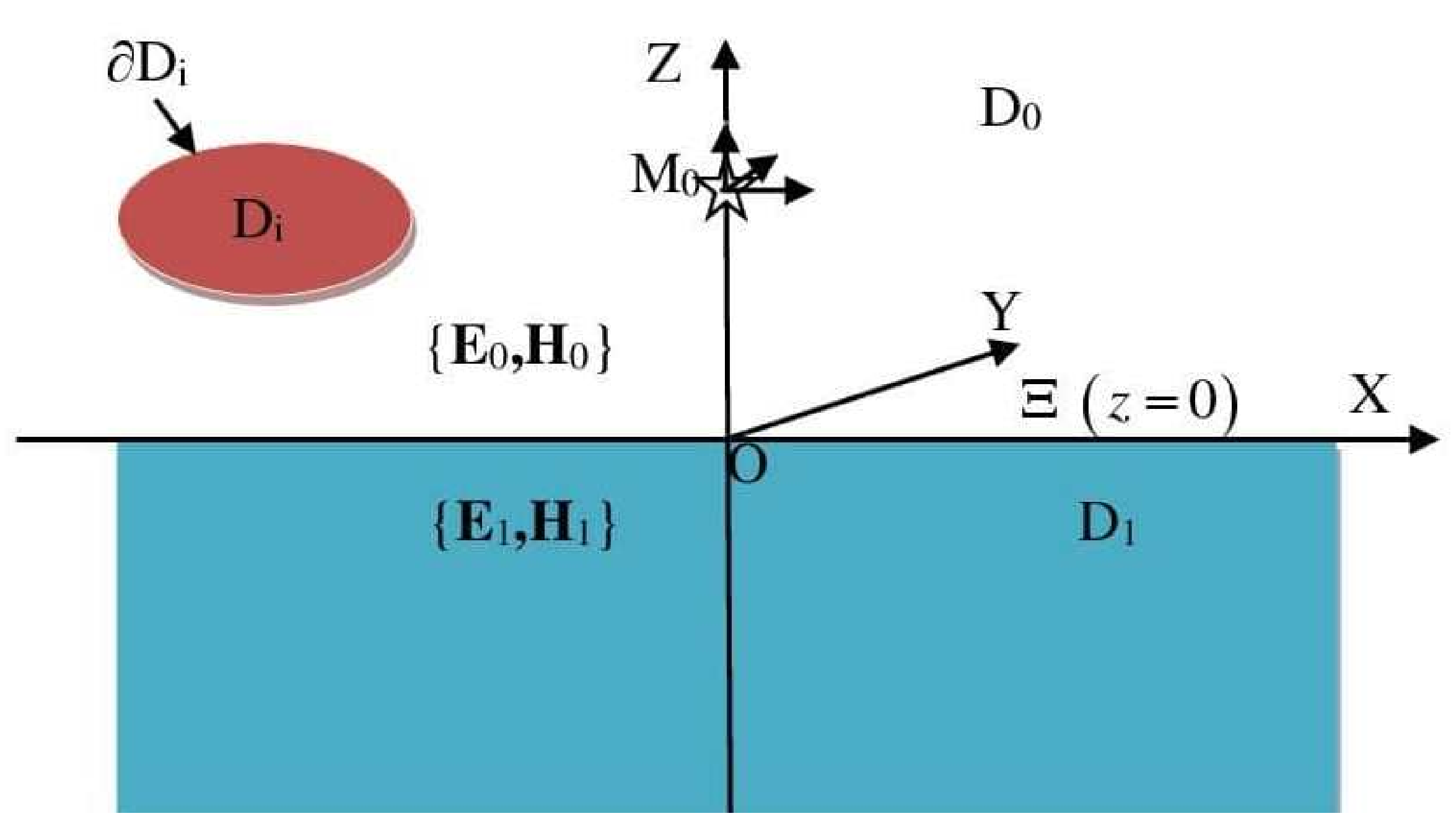
2.1. Boundary Value Problem Statement

Consider the excitation of a bounded isotropic penetrable particle $D_i$ with a smooth surface $\partial D_i$ by an electric multipole source of arbitrary order having a momentum p. A scheme of the considered scattering problem can be found in Figure 1.

Let the multipole be deposited at a point ${ \mathrm{M}}_0$, which is located outside of the particle $D_i$. The entire space ${ℝ}^3$ consists of two half-spaces, $D_0 \left(z>0\right)$ and $D_1 \left(z<0\right)$, separated by the plane interface $\mathsf{\Xi } \left(z=0\right)$. Assume that all media are nonmagnetic. Let the particle $D_i$ be located inside the upper half-space, $D_i\subset D_0$ and ${ \mathrm{M}}_0\in D_0$, too. Subsequently, the mathematical statement of the scattering problem can be written in the following form, including the time-harmonic Maxwell equations;

$$\nabla \times H_0=jk{\epsilon }_0{E}_0+J(M,M_0);\hspace{1em}\nabla \times E_0=-jk{H}_0 \mathrm{in} D_0;$$

$$\nabla \times H_l=jk{\epsilon }_l{E}_l;\begin{array}{cc}& \end{array}\hspace{1em}\nabla \times E_l=-jk{H}_l \mathrm{in} D_l,l=1,i;$$

the transmission conditions at the particle surface and plane interface;

$$\begin{array}{c}{n}_q\times \left(E_i(q)-E_0(q)\right)=0,\\ n_q\times \left(H_i(q)-H_0(q)\right)=0,\end{array} q\in \partial D_i,\begin{array}{c}{e}_z\times \left(E_1(Q)-E_0(Q)\right)=0,\\ e_z\times \left(H_1(Q)-H_0(Q)\right)=0,\end{array}\hspace{1em}\mathrm{Q}\in \mathsf{\Xi }$$

(1)

the Silver–Muller radiation conditions for all directions $r/r, z\ne 0$;

$$\underset{r\to \infty }{\lim } r\cdot \left(H_l\times \frac{r}{r}-\sqrt{{\epsilon }_l}{E}_l\right)=0,\hspace{1em}r=\left|M\right|\to \infty , l=0,1, z\ne 0;$$

and the additional infinity conditions along the interface $\mathsf{\Xi } \left(z=0\right)$ [19]

$$\max \left(\left|H_l\right|,\left|E_l\right|\right)=O({\rho }^{-\raisebox{1ex}{$1$}\!\left/ \!\raisebox{-1ex}{$2$}\right.}), \rho =\sqrt{x^2+y^2}, \rho \to \infty , z=\pm 0.$$

where the $\{E_l,H_l\}$—electric and magnetic fields in the corresponding domains $D_l, l=0,1,i$, $k=\omega /c$, $J=J(M,M_0)p$, $n_q$—unit external normal at $\partial D_i$, $e_z$—basic vector of the Cartesian coordinate system (x, y, z), axis OZ is orthogonal to Ξ. Assume that $\partial D_i\subset C^{(2,\alpha )}$ (Hölder space), the relative permittivity and permeability ${\epsilon }_i$ are continuous complex valued functions inside $D_i$ and $\mathrm{Im}{\epsilon }_i\le 0$, $\mathrm{Im}{\epsilon }_{0,1}=0$. The time dependence was chosen as $\exp \{\mathrm{j}\omega \mathrm{t}\}$. The corresponding radiation conditions were selected in such a form to provide uniqueness of the solution of the scattering problem (1).

Let us specify the $J(M,M_0)$ function. Choose the origin O of a Cartesian coordinate system and direct its Oz axis so that it passes through the point $M_0=\left(0,0,z_0\right)$ corresponding to the multipole position. Consider the multipole which, in a spherical coordinate system $\left(r,\theta ,\phi \right)$, accepts the following form:

$$w_n^m(M,M_0):=h_n^{(2)}(k_{0}r)P_n^m(\cos \theta )e^{-jm\phi };n=0,1,\dots ; m=0,\pm 1,\dots ; \left|m\right|\le n.$$

(2)

For the multipole (2), the following fundamental representation is valid [20]:

$$h_n^{(2)}(k_0{R}_{M{M}_0})P_n^m(\cos \theta )e^{-jm\phi }={(-1)}^m{j}^n{\left[\frac{j}{k_0}\left(\frac{\partial }{\partial x}-j\frac{\partial }{\partial y}\right)\right]}^m{P}_n^{(m)}\left(\frac{j}{k_0}\frac{\partial }{\partial z}\right)h_0^{(2)}(k_0{R}_{M{M}_0}),$$

here, $k_0=k\sqrt{{\epsilon }_0}$, $h_n^{(2)}(x)$ is a spherical Hankel function, $R_{M{M}_0}=\left|M-M_0\right|$, $P_n^{(m)}(\cos \theta )$ is an associated Legendre polynomial [21]. Introduce the following differential operator:

$$D_n^m={(-1)}^m{j}^{n-1}{\left[\frac{j}{k_0}{e}^{-j\phi }\frac{\partial }{\partial \rho }\right]}^m{P}_n^{(m)}\left(\frac{j}{k_0}\frac{\partial }{\partial z}\right).$$

(3)

taking into account the fundamental solution to the Helmholtz equation $\mathsf{\Psi }(M,M_0):$ $\mathsf{\Delta }\mathsf{\Psi }+k_0^2\mathsf{\Psi }=-\delta (M-M_0)$, which has the following form:

$\mathsf{\Psi }(M,M_0)=\frac{e^{-j{k}_0{R}_{M{M}_0}}}{4\pi R_{M{M}_0}}=-j\frac{k_0}{4\pi }{h}_0^{(2)}(k_0{R}_{M{M}_0})$, then

$\mathsf{\Delta }{w}_n^m+k_0^2{w}_n^m=\left(\mathsf{\Delta }+k_0^2\right)D_n^m\left\{j{h}_0^{(2)}(k_0{R}_{M{M}_0})\right\}=\frac{4\pi }{k_0}{D}_n^m\delta (M-M_0)$,

where δ—Dirac delta function. Subsequently, set up the $J(M,M_0)$ function in (1) as

$$J(M,M_0)=\frac{4\pi }{k_0}{D}_n^m\delta (M-M_0).$$

(4)

In this case, the scattering problem (1) has a unique solution [22]. In this case the electric field corresponding to the exciting multipole located at $M_0$ accepts the following form:

$$E_0^0(M)=-\frac{j}{k_0}\nabla \times \nabla \times \left\{w_n^m(M,M_0)p\right\}.$$

(5)

Now we are ready to proceed to the generalization of the optical theorem.

2.2. Generalization of the Optical Theorem

Choose a sphere $D_R$ of $R$—radius, centered at the plane Ξ and enclosing both $D_i$ and point $M_0$, and its boundary will be referred to as ${\mathsf{\Sigma }}_R$. The plane Ξ divides $D_R$ into two half-spheres $D_R^{\pm }$, deposited in $D_{0,1}$, and let ${\mathsf{\Sigma }}_R^{\pm }$ be parts of ${\mathsf{\Sigma }}_R$ belonging to $D_R^{\pm }$, respectively. The application of the Gauss divergence theorem [22] to the solution of the problem (1) of the total electric $E_0$ and the complex conjugate magnetic $H_0^{\ast }$ fields in the domain $D_R^{+}/{\overline{D}}_i$ allows us to obtain the following formula:

$$\begin{array}{l} {\displaystyle \underset{D_R^{+}/{\overline{D}}_i}{\int }\nabla \cdot \left[E_0\times H_0^{\ast }\right]}d\tau ={\displaystyle \underset{D_R^{+}/{\overline{D}}_i}{\int }\left\{H_0^{\ast }\cdot \nabla \times E_0-E_0\cdot \nabla \times H_0^{\ast }\right\}}d\tau =\\ ={\displaystyle \underset{D_R^{+}/{\overline{D}}_i}{\int }\left\{jk\left(-{\left|H_0^{\ast }\right|}^2+{\left|E_0\right|}^2\right)-(E_0\cdot J_{}^{\ast })\right\}}d\tau ={\displaystyle \underset{{\mathsf{\Sigma }}_R^{+}\cup {\mathsf{\Xi }}_R\cup \partial D_i}{\int }\left[E_0\times H_0^{\ast }\right]}\cdot ds,\end{array}$$

(6)

where ${\mathsf{\Xi }}_R:=\left\{M\in \mathsf{\Xi } : \left|M\right|\le R\right\}$ is a part of the plane $\mathsf{\Xi }$. Taking the real parts from both sides of (6) and rewriting the integrals in the right part we obtain the following formula:

$$\begin{array}{l}\mathrm{Re}{\displaystyle \underset{\partial D_i}{\int }\left[E_0\times H_0^{\ast }\right]}\cdot d\sigma +\mathrm{Re}{\displaystyle \underset{{\mathsf{\Sigma }}_R^{+}}{\int }\left[E_0\times H_0^{\ast }\right]}\cdot \frac{r}{r}d\sigma -\mathrm{Re}{\displaystyle \underset{{\mathsf{\Xi }}_R}{\int }\left[E_0\times H_0^{\ast }\right]}\cdot e_{z}d\sigma =\\ -\mathrm{Re}{\displaystyle \underset{D_R^{+}/{\overline{D}}_i}{\int }(E_0\cdot J^{\ast })}d\tau ,\end{array}$$

(7)

A similar application of Gauss’s theorem inside $D_i$ leads to the following:

$$\mathrm{Re}{\displaystyle \underset{\partial D_i}{\int }\left[E_i\times H_i{}^{\ast }\right]}\cdot d\sigma =k{\displaystyle \underset{D_i}{\int }\left\{\left|\mathrm{Im}{\epsilon }_i\right|{\left|E_i\right|}^2\right\}}d\tau .$$

(8)

The right part of (8) will be referred to as the absorption cross-section $C_{abs}$ and, subsequently, (7) accepts the following form:

$$C_{abs}+\mathrm{Re}{\displaystyle \underset{{\mathsf{\Sigma }}_R^{+}}{\int }\left[E_0\times H_0^{\ast }\right]}\cdot \frac{r}{r}d\sigma -\mathrm{Re}{\displaystyle \underset{{\mathsf{\Xi }}_R}{\int }\left[E_0\times H_0^{\ast }\right]}\cdot e_{z}d\sigma =-\mathrm{Re}{\displaystyle \underset{D_R^{+}/{\overline{D}}_i}{\int }(E_0\cdot J^{\ast })}d\tau .$$

(9)

Using Gauss’s theorem in the $D_R^{-}$ domain and taking the real part, we obtain the following formula:

$$\mathrm{Re}{\displaystyle \underset{{\mathsf{\Sigma }}_R^{-}}{\int }\left[E_1\times H_1^{\ast }\right]}\cdot \frac{r}{r}d\sigma +\mathrm{Re}{\displaystyle \underset{{\mathsf{\Xi }}_R}{\int }\left[E_1\times H_1^{\ast }\right]}\cdot e_{z}d\sigma =0.$$

(10)

Combining equations (9) and (10) yields the following:

$$C_{abs}+\mathrm{Re}{\displaystyle \underset{{\mathsf{\Sigma }}_R^{+}}{\int }\left[E_0\times H_0^{\ast }\right]}\cdot \frac{r}{r}d\sigma +\mathrm{Re}{\displaystyle \underset{{\mathsf{\Sigma }}_R^{-}}{\int }\left[E_1\times H_1^{\ast }\right]}\cdot \frac{r}{r}d\sigma =-\mathrm{Re}{\displaystyle \underset{D_R^{+}/{\overline{D}}_i}{\int }(E_0\cdot J^{\ast })}d\tau .$$

(11)

Subsequently, consider the far-field patterns $F_{0,1}(\theta ,\phi )$ of the fields [22] in the upper and lower half-spaces $D_R^{\pm }$

$$E_{0,1}(M)=\frac{e^{-jk{n}_{0,1}r}}{r}{F}_{0,1}(\theta ,\phi )+o(\frac{1}{r}),r\to \infty ,z\ne 0.$$

The far-field patterns are defined at the upper and lower unit hemi-spheres ${\mathsf{\Omega }}^{+}=\left\{0\le \phi \le {360}^{\circ };0\le \theta <{90}^{\circ }\right\}$, ${\mathsf{\Omega }}^{-}=\left\{0\le \phi \le {360}^{\circ };{90}^{\circ }<\theta \le {180}^{\circ }\right\}$, where $n_{0,1}=\sqrt{{\epsilon }_{0,1}}$. Then, having a radius R tending toward infinity leads to the following:

$$\begin{array}{l}\underset{R\to \infty }{\lim }\mathrm{Re}{\displaystyle \underset{{\mathsf{\Sigma }}_R^{+}}{\int }\left[E_0\times H_0^{\ast }\right]}\cdot \frac{r}{r}d\sigma =\mathrm{Re}\underset{R\to \infty }{\lim }{\displaystyle \underset{{\mathsf{\Sigma }}_R^{+}}{\int }{E}_0\cdot \left[H_0^{\ast }\times \frac{r}{r}\right]}d\sigma =\\ \sqrt{{\epsilon }_0}\underset{R\to \infty }{\lim }{{\displaystyle \underset{{\mathsf{\Sigma }}_R^{+}}{\int }\left|E_0\right|}}^{2}d\sigma =\sqrt{{\epsilon }_0}{\displaystyle \underset{{\mathsf{\Omega }}^{+}}{\int }{\left|F_0\right|}^{2}d\omega }.\end{array}$$

Similarly, for the lower half-space $D_1$:

$$\begin{array}{l}\underset{R\to \infty }{\lim }\mathrm{Re}{\displaystyle \underset{{\mathsf{\Sigma }}_R^{-}}{\int }\left[E_1\times H_1^{\ast }\right]}\cdot \frac{r}{r}d\sigma =\mathrm{Re}\underset{R\to \infty }{\lim }{\displaystyle \underset{{\mathsf{\Sigma }}_R^{-}}{\int }{E}_1\cdot \left[H_1^{\ast }\times \frac{r}{r}\right]}d\sigma \\ =\sqrt{{\epsilon }_1}\underset{R\to \infty }{\lim }{{\displaystyle \underset{{\mathsf{\Sigma }}_R^{-}}{\int }\left|E_1\right|}}^{2}d\sigma =\sqrt{{\epsilon }_1}{\displaystyle \underset{{\mathsf{\Omega }}^{-}}{\int }{\left|F_1\right|}^{2}d\omega .}\end{array}$$

The last integrals can be referred to as the scattering cross-sections in the upper and the lower half-spaces $D_{0,1}$—$C_{sc}^{\pm }$. Therefore, (11) can be rewritten in a simple form:

$$C_{abs}+C_{sc}^{+}+C_{sc}^{-}=-\mathrm{Re}{\displaystyle \underset{D_0/{\overline{D}}_i}{\int }(E_0\cdot J^{\ast })}d\tau .$$

(12)

It is worth noting that the scattering cross-sections $C_{sc}^{\pm }$ include a part associated to the multipole radiation patterns. Represent the total fields in $D_R^{\pm }$ as $E_{0,1}=E_{0,1}^s+E_{0,1}^d$, where $E_{0,1}^d$ is the field corresponding to the radiating multipole located at $M_0$, and $E_{0,1}^s$ is the scattered field corresponding only to the particle $D_i$. Because the total field $E_{0,1}$ satisfies the transmission conditions at the plane interface Ξ, both $E_{0,1}^s$ and $E_{0,1}^d$ should obey the same transmission conditions. We continue the transformation of the integral in the right part of (12) and, by employing the δ-function properties [23], we then account for [17]

$$\begin{array}{l}{\displaystyle \underset{D_0/{\overline{D}}_i}{\int }(E_0\cdot J^{\ast })}d\tau ={\displaystyle \underset{D_0/{\overline{D}}_i}{\int }\left(E_0^s(Q)+E_0^d(Q)\right)\cdot p{J}^{\ast }(Q,M_0)}d{\tau }_Q=\frac{4\pi }{k_0}{\displaystyle \underset{D_0/{\overline{D}}_i}{\int }{D}_n^{m\ast }\delta (Q-M_0)E_0^s(Q)\cdot p}d{\tau }_Q\\ +{\displaystyle \underset{D_0/{\overline{D}}_i}{\int }{E}_0^d(Q)\cdot p{J}^{\ast }(Q,M_0)}d{\tau }_Q={\displaystyle \underset{D_0/{\overline{D}}_i}{\int }{J}^{\ast }(Q,M_0)E_0^d(Q)\cdot p}d{\tau }_Q+\frac{4\pi }{k_0}{\left[D_n^{m+}\left(E_0^s(M)\cdot p\right)\right]}_{M=M_0}.\end{array}$$

(13)

The last term has already been obtained in [17]. Here, $D_n^{m+}$ is Hermitian conjugate operator, with respect to (3) having the following form:

$$D_n^{m+}={(-1)}^{m-1}{j}^{n-1}{\left[\frac{j}{k_0}{e}^{j\phi }\frac{\partial }{\partial \rho }\right]}^m{P}_n^{(m)}\left(\frac{j}{k_0}\frac{\partial }{\partial z}\right),$$

(14)

Here, $P_n^{(m)}(-x)={(-1)}^{n+m}{P}_n^{(m)}(x)$ [21]. It should be remembered that $E_0^s$ is an analytic function in the region $D_0$ [22]. To evaluate the first integral in the right part of (13), we need a representation for the electric multipole field satisfying the transmission conditions at the interface Ξ. This can be obtained based on the electric green tensor (GT) of half-space ${\overleftrightarrow{G}}^e(M,M_0)$, which can be written in the form [24]

$${\overleftrightarrow{G}}^e(M,M_0)=\left[\begin{array}{ccc}{G}_{11}^{}& 0& 0\\ 0& G_{11}^{}& 0\\ \partial g/\partial x_M& \partial g/\partial y_M& G_{33}^{}\end{array}\right].$$

(15)

The GT components in $D_{0,1}$ have the following representations:

$$G_{ll}(M,M_0)={\displaystyle \underset{0}{\overset{\infty }{\int }}{J}_0(\lambda r) v_{ll}(\lambda ,z,z_0)\lambda d\lambda } , l=1,3; g(M,M_0)={\displaystyle \underset{0}{\overset{\infty }{\int }}{J}_0(\lambda r) v_{31}(\lambda ,z,z_0)\lambda d\lambda },$$

where $r^2={(x-x_0)}^2+{(y-y_0)}^2$, $J_0$—cylindrical Bessel function [21], $(x_0,y_0,z_0)$—Cartesian coordinates of point $M_0$. The corresponding spectral functions $v_{11},v_{33},v_{31}$ fulfilling the transmission conditions at $z=0$ can be found in Appendix A (see formulas (A1) and(A2)).

Following the multipole definition, consider the multipole representation for the GT by extracting the singular part as:

$${\overleftrightarrow{W}}_n^m(M,M_0)=\frac{4\pi }{k_0}{D}_n^m\overleftrightarrow{G^e}(M,M_0)=w_n^m(M,M_0)\cdot I+\frac{4\pi }{k_0}{D}_n^m\overleftrightarrow{G_r^e}(M,M_0),$$

(16)

where $\overleftrightarrow{G_r^e}(M,M_0)$ is the regular part of the GT multipole representation, I—idem factor. Subsequently, the corresponding electric field of the multipole in $D_0$ appears as:

$$E_0^d(M)=E_0^0(M)-\frac{4\pi j}{k_0^2}\nabla \times \nabla \times \left\{D_n^m\overleftrightarrow{G_r^e}(M,M_0)p\right\}=E_0^0(M)+E_0^r(M).$$

(17)

Then,

$$\begin{array}{l}-\mathrm{Re}{\displaystyle \underset{D_0/{\overline{D}}_i}{\int }{J}^{\ast }(Q,M_0)E_0^d(Q)\cdot p}d{\tau }_Q=\\ \begin{array}{ccc}& & \end{array}-\mathrm{Re}{\displaystyle \underset{D_0/{\overline{D}}_i}{\int }{J}^{\ast }(Q,M_0)E_0^0(Q)\cdot p}d{\tau }_Q-\mathrm{Re}{\displaystyle \underset{D_0/{\overline{D}}_i}{\int }{J}^{\ast }(Q,M_0)E_0^r(Q)\cdot p}d{\tau }_Q.\end{array}$$

The first integral represents the total energy irradiated by a multipole deposited in free space. This integral is examined in detail in [25]. Let the polarization vector have the Cartesian coordinates $p=\left(p_x,p_y,p_z\right)$, then the first integral can be written as

$$-\mathrm{Re}{\displaystyle \underset{D_0/{\overline{D}}_i}{\int }{J}^{\ast }(Q,M_0)E_0^0(Q)\cdot p}d{\tau }_Q=\frac{\pi }{k_0^2}\left\{\left[\frac{2}{3}{\beta }_n^m+\frac{1}{3}\right]\left(p_x^2+p_y^2\right)+\left[\frac{2}{3}-\frac{2}{3}{\beta }_n^m\right]p_z^2\right\}{‖P_n^m‖}^2.$$

(18)

Substituting a specific expression for $J(Q,M_0)$: (4) and $E_0^0(Q)$: (5); taking into account that ${{\displaystyle \underset{-1}{\overset{1}{\int }}{P}_2^0(x)\left[P_n^m(x)\right]}}^{2}dx={\beta }_n^m{‖P_n^m‖}^2$ and following [25] we obtain (18), where ${\beta }_n^m=C(nn2,000)C(nn2,mm0),$ $C(\dots ,\dots )$ are Clebsch–Gordan coefficients, and ${‖P_n^m‖}^2$ is the norm of associated Legendre polynomials [21] ${‖P_n^m‖}^2=\frac{2}{2n+1}\frac{\left(n+m\right)!}{\left(n-m\right)!}$. Unfortunately, Clebsch–Gordan coefficients do not have an explicit analytical representation for an arbitrary integer $n,m$ but they can be estimated numerically.

Consider the integral containing the regular field in the right part of the last relation. We start from its z-component, then

$$p_z\cdot \nabla \times \nabla \times \left\{D_n^m{\overleftrightarrow{G}}_r^e(M,M_0)p_z\right\}={\left|p_z\right|}^2{D}_n^m\left\{k_0^2{\overline{G}}_{33}(M,M_0)+\frac{{\partial }^2}{\partial z^2}{\overline{G}}_{33}(M,M_0)\right\}.$$

By substituting the representation for the current into the integral, we obtain the following formula:

$$\begin{array}{cc}\hfill & \underset{D_0/{\overline{D}}_i}{\int }{J}^{*}{\mathbf{E}}_0^r{\mathbf{p}}_{z}d\tau \hfill \\ \hfill & =\frac{4\pi j}{k_0^2}{\left|{\mathbf{p}}_z\right|}^2{D}_n^{m+}{D}_n^m\underset{D_0/{\overline{D}}_i}{\int }\underset{0}{\overset{\infty }{\int }}{A}_{33}{J}_0\left(\lambda \rho \right)\left(k_0^2+\frac{{\partial }^2}{\partial z^2}\right)\frac{exp\left\{-{\eta }_{0}z\right\}}{{\eta }_0}\lambda d\lambda \delta (Q-M_0)d{\tau }_Q\hfill \\ \hfill & =\frac{4\pi j}{k_0^2}{\left|{\mathbf{p}}_z\right|}^2\underset{D_0/{\overline{D}}_i}{\int }\underset{0}{\overset{\infty }{\int }}{A}_{33}(\lambda ,z_0)D_n^{m+}{D}_n^m{J}_0\left(\lambda \rho \right)\frac{exp\left\{-{\eta }_{0}z\right\}}{{\eta }_0}{\lambda }^{3}d\lambda \delta (Q-M_0)d{\tau }_Q.\hfill \end{array}$$

(19)

It is worth noting that the multipole is located at the 0z axis, $M_0=(0,0,z_0)$. It can then be realized that

$$D_n^{m+}{D}_n^m=\frac{1}{k_0^{2m}}\frac{{\partial }^{2m}}{\partial {\rho }^{2m}}{\left[P_n^{(m)}(\frac{j}{k_0}\frac{\partial }{\partial z})\right]}^2.$$

By applying this operator to the integrand of the integral in the right part of (19), the following can be expressed:

$${\left\{\frac{{\partial }^{2m}}{\partial {\rho }^{2m}}{J}_0(\lambda \rho )\right\}}_{\rho =0}{\left\{{\left[P_n^{(m)}(\frac{j}{k_0}\frac{\partial }{\partial z})\right]}^2\frac{\exp \left\{-{\eta }_{0}z\right\}}{{\eta }_0}\right\}}_{z=z_0},$$

and accounting for $J_0(\lambda \rho )={\displaystyle \sum _{l=0}^{\infty }\frac{{(-1)}^l}{{(l!)}^2}}{\left(\frac{\lambda \rho }{2}\right)}^{2l}$ [21], that the following can be presented:

$$\begin{array}{l}{\left\{\frac{{\partial }^{2m}}{\partial {\rho }^{2m}}{J}_0(\lambda \rho )\right\}}_{\rho =0}{\left\{{\left[P_n^{(m)}(\frac{j}{k_0}\frac{\partial }{\partial z})\right]}^2\frac{\exp \left\{-{\eta }_{0}z\right\}}{{\eta }_0}\right\}}_{z=z_0}=\\ \begin{array}{cc}& \end{array}\frac{{(-1)}^m{\lambda }^{2m}\left(2m-1\right)!!}{\left(2m\right)!!}{\left[P_n^{(m)}(\frac{j}{k_0}{\eta }_0)\right]}^2\frac{\exp \left\{-{\eta }_0{z}_0\right\}}{{\eta }_0}.\end{array}$$

By substituting the formula for $A_{33}$: (A4) we obtain the following:

$$\begin{array}{l}{\displaystyle \underset{D_0/{\overline{D}}_i}{\int }{J}^{\ast }(Q,M_0)E_0^r(Q)p_z}d{\tau }_Q=\\ \begin{array}{cc}& \end{array}\frac{4\pi j{\left|p_z\right|}^2\left(2m-1\right)!!}{k_0^{2m+2}\left(2m\right)!!}{\displaystyle \underset{0}{\overset{\infty }{\int }}\frac{{\epsilon }_1{\eta }_0-{\epsilon }_0{\eta }_1}{{\epsilon }_1{\eta }_0+{\epsilon }_0{\eta }_1}{\left[P_n^{(m)}(\frac{j}{k_0}{\eta }_0)\right]}^2\frac{\exp \left\{-2{\eta }_0{z}_0\right\}}{{\eta }_0}{\lambda }^{2m+3}d\lambda }\end{array}$$

(20)

By taking the real part of the integral, we obtain the following:

$$\begin{array}{l}-\mathrm{Re}{\displaystyle \underset{D_0/{\overline{D}}_i}{\int }{J}^{\ast }{E}_0^r\cdot p_z}d{\tau }_Q=\\ \begin{array}{cc}& \end{array}\frac{4\pi {\left|p_z\right|}^2\left(2m-1\right)!!}{k_0^{2m+2}\left(2m\right)!!}\mathrm{Im}{\displaystyle \underset{0}{\overset{\infty }{\int }}\frac{{\epsilon }_1{\eta }_0-{\epsilon }_0{\eta }_1}{{\epsilon }_1{\eta }_0+{\epsilon }_0{\eta }_1}{\left[P_n^{(m)}(\frac{j}{k_0}{\eta }_0)\right]}^2\frac{\exp \left\{-2{\eta }_0{z}_0\right\}}{{\eta }_0}{\lambda }^{2m+3}d\lambda .}\end{array}$$

(21)

Consider the integrand in (21) following to [26]. It is clear that under $\lambda >\max (k_0,k_1)$ we have $\mathrm{Im}{\eta }_{0,1}=0$. Based on the properties of $P_n^{(m)}(jx)$ under $\mathrm{Im}x=0$, depending on the specific integer values of $n,m$, the following correlations are relevant: either $\mathrm{Re}{P}_n^{(m)}(jx)=0$, or $\mathrm{Im}{P}_n^{(m)}(jx)=0$. Hence, $\mathrm{Im}{\left[P_n^{(m)}(j\frac{{\eta }_0}{k_0})\right]}^2\equiv 0$ for $\forall n,m, n\in \mathbb{N}, n\ge m$, and $\lambda >\max (k_0,k_1)$. Therefore, for all real valued $k_1>k_0$, we obtain the following:

$$\begin{array}{l}-\mathrm{Re}{\displaystyle \underset{D_0/{\overline{D}}_i}{\int }{J}^{\ast }{E}_0^r\cdot p_z}d{\tau }_Q=\\ \begin{array}{cc}& \end{array}\frac{4\pi {\left|p_z\right|}^2(2m-1)!!}{k_0^{2m+2}(2m)!!}\mathrm{Im}{\displaystyle \underset{0}{\overset{k_1}{\int }}\frac{{\epsilon }_1{\eta }_0-{\epsilon }_0{\eta }_1}{{\epsilon }_1{\eta }_0+{\epsilon }_0{\eta }_1}{\left[P_n^{(m)}(\frac{j}{k_0}{\eta }_0)\right]}^2\frac{\exp \left\{-2{\eta }_0{z}_0\right\}}{{\eta }_0}{\lambda }^{2m+3}d\lambda .}\end{array}$$

(22)

We continue to analyze the regular field x-component in the same manner:

$$\begin{array}{l}{p}_x\cdot \nabla \times \nabla \times \left\{D_n^m{\overleftrightarrow{G}}_r^e(M,M_0)p_x\right\}=p_x\cdot \nabla \times \nabla \times D_n^m\left\{{\overline{G}}_{11}(M,M_0)+\frac{\partial }{\partial x}g(M,M_0)\right\}\cdot p_x=\\ \frac{4\pi j}{k_0^2}{\left|p_x\right|}^2{D}_n^m\left\{k_0^2\left[{\overline{G}}_{11}(M_0,M_0)+\frac{\partial }{\partial x}g(M,M_0)\right]+\left[\frac{{\partial }^2}{\partial x^2}{\overline{G}}_{11}(M_0,M_0)+\frac{{\partial }^3}{\partial x^3}g(M,M_0)\right]\right\}.\end{array}$$

(23)

It should be remembered that the presence of any odd order derivatives with respect to x or y of the integral containing $J_0(\lambda r)$ leads to the nullification of the result at $M=M_0 (r=0)$. This can be easily observed from the series for the Bessel function of zero order, which contains only even powers of argument. Subsequently, the relation (23) can be written as the following formula:

$$p_x\cdot \nabla \times \nabla \times \left\{D_n^m\overleftrightarrow{G_r^e}(M,M_0)p_x\right\}=\frac{4\pi j}{k_0^2}{\left|p_x\right|}^2{D}_n^m\left\{k_0^2{\overline{G}}_{11}(M_0,M_0)+\frac{{\partial }^2}{\partial x^2}{\overline{G}}_{11}(M_0,M_0)\right\}.$$

Let us proceed to the consideration of the x-component, that is:

$$\begin{array}{l}\begin{array}{cc}& \end{array}{\displaystyle \underset{D_0/{\overline{D}}_i}{\int }{J}^{\ast }{E}_0^r{p}_x}d\tau =\\ \begin{array}{ccc}& & \end{array}\frac{4\pi j}{k_0^2}{\left|p_x\right|}^2{D}_n^{m+}{D}_n^m{\displaystyle \underset{D_0/{\overline{D}}_i}{\int }{\displaystyle \underset{0}{\overset{\infty }{\int }}{A}_{11}(\lambda ,z_0)\left(k_0^2+\frac{{\partial }^2}{\partial x^2}\right)J_0(\lambda \rho )\frac{\exp \left\{-{\eta }_{0}z\right\}}{{\eta }_0}\lambda d\lambda }}\delta (Q-M_0)d{\tau }_Q.\end{array}$$

(24)

Following our previous consideration for the z-component (22) and the explicit formula for $A_{11}$: (A3), we can present the following:

$$\begin{array}{cc}\hfill & \underset{D_0/{\overline{D}}_i}{\int }{J}^{*}{\mathbf{E}}_0^r{\mathbf{p}}_{x}d\tau \hfill \\ \hfill & =\frac{4\pi j}{k_0^2}{\left|{\mathbf{p}}_x\right|}^2{D}_n^{m+}{D}_n^m\underset{D_0/{\overline{D}}_i}{\int }\underset{0}{\overset{\infty }{\int }}{A}_{11}\left(k_0^2+\frac{{\partial }^2}{\partial x^2}\right)J_0\left(\lambda \rho \right)\frac{exp\left\{-{\eta }_{0}z\right\}}{{\eta }_0}\lambda d\lambda \delta (Q-M_0)d{\tau }_Q\hfill \\ \hfill & =\frac{4\pi j{\left|{\mathbf{p}}_x\right|}^2\left(2m\right)!}{k_0^{2m}{\left[\left(2m\right)!!\right]}^2}\underset{0}{\overset{\infty }{\int }}\frac{{\eta }_0-{\eta }_1}{{\eta }_0+{\eta }_1}{\left[P_n^{\left(m\right)}\left(\frac{j}{k_0}{\eta }_0\right)\right]}^2\frac{exp\left\{-2{\eta }_0{z}_0\right\}}{{\eta }_0}{\lambda }^{2m+1}d\lambda +\hfill \\ \hfill & +\frac{4\pi j}{k_0^2}{\left|{\mathbf{p}}_x\right|}^2\underset{0}{\overset{\infty }{\int }}{A}_{11}(\lambda ,z_0){\left\{\frac{{\partial }^{2m}}{\partial {\rho }^{2m}}\frac{{\partial }^2}{\partial x^2}{J}_0\left(\lambda \rho \right)\right\}}_{\rho =0}{\left\{{\left[P_n^{\left(m\right)}\left(\frac{j}{k_0}\frac{\partial }{\partial z}\right)\right]}^2\frac{exp\left\{-{\eta }_{0}z\right\}}{{\eta }_0}\right\}}_{z=z_0}\lambda d\lambda .\hfill \end{array}$$

(25)

Then, the last integral in the previous relation (25) can be transformed as:

$$\begin{array}{l}{\displaystyle \underset{0}{\overset{\infty }{\int }}\frac{{\eta }_0-{\eta }_1}{{\eta }_0+{\eta }_1}{\zeta }_0{\left\{\frac{{\partial }^{2m}}{\partial {\rho }^{2m}}\frac{{\partial }^2}{\partial x^2}{J}_0(\lambda \rho )\right\}}_{\rho =0}{\left\{{\left[P_n^{(m)}(\frac{j}{k_0}\frac{\partial }{\partial z})\right]}^2\frac{\exp \left\{-{\eta }_{0}z\right\}}{{\eta }_0}\right\}}_{z=z_0}\lambda d\lambda }=\\ -\frac{(2m+1)!!}{k_0^{2m}(2m+2)!!}{\displaystyle \underset{0}{\overset{\infty }{\int }}\frac{{\eta }_0-{\eta }_1}{{\eta }_0+{\eta }_1}{\left[P_n^{(m)}(\frac{j}{k_0}{\eta }_0)\right]}^2\frac{\exp \left\{-2{\eta }_0{z}_0\right\}}{{\eta }_0}{\lambda }^{2m+3}d\lambda }.\end{array}$$

The collection of the two previously obtained relations allows us to conclude that

$$\begin{array}{cc}\hfill & \underset{D_0/{\overline{D}}_i}{\int }{J}^{*}{\mathbf{E}}_0^r{\mathbf{p}}_{x}d\tau =\frac{4\pi j{\left|{\mathbf{p}}_x\right|}^2(2m-1)!!}{k_0^{2m}\left(2m\right)!!}\underset{0}{\overset{\infty }{\int }}\frac{{\eta }_0-{\eta }_1}{{\eta }_0+{\eta }_1}{\left[P_n^{\left(m\right)}\left(\frac{j}{k_0}{\eta }_0\right)\right]}^2\frac{exp\left\{-2{\eta }_0{z}_0\right\}}{{\eta }_0}{\lambda }^{2m+1}d\lambda -\hfill \\ \hfill & -\frac{4\pi j{\left|{\mathbf{p}}_x\right|}^2(2m+1)!!}{k_0^{2m+2}\left(2m+2\right)!!}\underset{0}{\overset{\infty }{\int }}\frac{{\eta }_0-{\eta }_1}{{\eta }_0+{\eta }_1}{\left[P_n^{\left(m\right)}\left(\frac{j}{k_0}{\eta }_0\right)\right]}^2\frac{exp\left\{-2{\eta }_0{z}_0\right\}}{{\eta }_0}{\lambda }^{2m+3}d\lambda =\hfill \\ \hfill & \frac{4\pi j{\left|{\mathbf{p}}_x\right|}^2(2m-1)!!}{k_0^{2m+2}\left(2m\right)!!}\underset{0}{\overset{\infty }{\int }}\frac{{\eta }_0-{\eta }_1}{{\eta }_0+{\eta }_1}\left(k_0^2-{\lambda }^2\frac{(2m+1)}{(2m+2)}\right){\left[P_n^{\left(m\right)}\left(\frac{j}{k_0}{\eta }_0\right)\right]}^2\frac{exp\left\{-2{\eta }_0{z}_0\right\}}{{\eta }_0}{\lambda }^{2m+1}d\lambda .\hfill \end{array}$$

(26)

Obtaining the real part from both sides of (26) and accounting for (22), we finally apprehend the following

$$\begin{array}{l}-\mathrm{Re}{\displaystyle \underset{D_0/{\overline{D}}_i}{\int }{J}^{\ast }(Q,M_0)E_0^r(Q)\cdot p_x}d{\tau }_Q=\\ \begin{array}{cc}& \end{array}\frac{4\pi {\left|p_x\right|}^2(2m-1)!!}{k_0^{2m+2}\left(2m\right)!!}\mathrm{Im}{\displaystyle \underset{0}{\overset{k_1}{\int }}\frac{{\eta }_0-{\eta }_1}{{\eta }_0+{\eta }_1}\left(k_0^2-{\lambda }^2\frac{(2m+1)}{(2m+2)}\right){\left[P_n^{(m)}(\frac{j}{k_0}{\eta }_0)\right]}^2\frac{\exp \left\{-2{\eta }_0{z}_0\right\}}{{\eta }_0}{\lambda }^{2m+1}d\lambda .}\end{array}$$

(27)

It is clear that, for the y-component, we can obtain a similar representation.

3. Results

In the previous section, we completed all preliminary considerations and are ready to formulate the main result.

Theorem 1.

Let us consider the boundary value problem of excitation (1) of a penetrable scatterer deposited above a transparent substrate by a multipole of arbitrary order (4) and polarization p = (p_x,p_y,p_z), localized at the point M₀ = (0,0,z₀) of the Cartesian coordinate system. Then, the extinction cross-section$C_{ext}:=C_{scs}+C_{abs}$[27] accepts the following form:

$$\begin{array}{cc}\hfill & C_{ext}=-\frac{4\pi }{k_0}Re{\left[D_n^{m+}\left({\mathbf{E}}_0^s\left(M\right)·\mathbf{p}\right)\right]}_{M=M_0}+\frac{\pi }{k_0^2}\left\{\left[\frac{2}{3}{\beta }_n^m+\frac{1}{3}\right]\left(p_x^2+p_y^2\right)+\left[\frac{2}{3}-\frac{2}{3}{\beta }_n^m\right]p_z^2\right\}{∥P_n^m∥}^2+\hfill \\ \hfill & \frac{4\pi p_z^2(2m-1)!!}{k_0^{2m+2}\left(2m\right)!!}Im\underset{0}{\overset{k_1}{\int }}\frac{{\epsilon }_1{\eta }_0-{\epsilon }_0{\eta }_1}{{\epsilon }_1{\eta }_0+{\epsilon }_0{\eta }_1}{\left[P_n^{\left(m\right)}\left(\frac{j}{k_0}{\eta }_0\right)\right]}^2\frac{exp\left\{-2{\eta }_0{z}_0\right\}}{{\eta }_0}{\lambda }^{2m+3}d\lambda +\hfill \\ \hfill & \frac{4\pi \left(p_x^2+p_y^2\right)(2m-1)!!}{k_0^{2m+2}\left(2m\right)!!}Im\underset{0}{\overset{k_1}{\int }}\frac{{\eta }_0-{\eta }_1}{{\eta }_0+{\eta }_1}\left(k_0^2-{\lambda }^2\frac{(2m+1)}{(2m+2)}\right){\left[P_n^{\left(m\right)}\left(\frac{j}{k_0}{\eta }_0\right)\right]}^2\frac{exp\left\{-2{\eta }_0{z}_0\right\}}{{\eta }_0}{\lambda }^{2m+1}d\lambda .\hfill \end{array}$$

(28)

It is can clearly be observed that, in case of an absence of the substrate ${\epsilon }_1={\epsilon }_0\Rightarrow k_1=k_0\Rightarrow {\eta }_1={\eta }_0$, the Formula (28) is reduced to the following:

$$C_{ext}^0=-\frac{4\pi }{k_0}\mathrm{Re}{\left[D_n^{m+}\left(E_0^s(M)\cdot p\right)\right]}_{M=M_0}+\frac{\pi }{k_0^2}\left\{\left[\frac{2}{3}{\beta }_n^m+\frac{1}{3}\right]\left(p_x^2+p_y^2\right)+\left[\frac{2}{3}-\frac{2}{3}{\beta }_n^m\right]p_z^2\right\}{‖P_n^m‖}^2,$$

(29)

which represents the OT for multipole excitations of a particle in free space [25].

Let us consider a specific case: excitation by a vertical electric quadrupole $p_x=p_y=0$ deposited in $M_0=\left(0,0,z_0\right)$. This case corresponds to $m=0, n=1$. Subsequently,

$$D_1^0=P_1(\frac{j}{k_0}\frac{\partial }{\partial z})=\frac{j}{k_0}\frac{\partial }{\partial z}.$$

Using an estimate of the second term in (29), and then following [25], we obtain the following:

$${\displaystyle \underset{0}{\overset{\pi }{\int }}\left[P_1(\cos \theta )\right]{\sin }^2\theta \sin \theta d\theta ={\displaystyle \underset{-1}{\overset{1}{\int }}{x}^2(1-x^2)}}dx=\frac{4}{15}.$$

Considering that $D_1^{0+}=-\frac{j}{k_0}\frac{\partial }{\partial z}$, Formula (29) can be rewritten as

$$C_{ext}^0=\frac{4\pi }{k_0^2}\mathrm{Im}{\left[p_z\cdot \frac{\partial }{\partial z}{E}_0^s(M)\right]}_{M=M_0}+\frac{4\pi }{15k_0^2}.$$

(30)

We subsequently transform the corresponding integral in (28) as

$$\begin{array}{l}\frac{4\pi p_z^2}{k_0^2}\mathrm{Im}{\displaystyle \underset{0}{\overset{k_1}{\int }}\frac{{\epsilon }_1{\eta }_0-{\epsilon }_0{\eta }_1}{{\epsilon }_1{\eta }_0+{\epsilon }_0{\eta }_1}{\left[\frac{j}{k_0}{\eta }_0\right]}^2\frac{\exp \left\{-2{\eta }_0{z}_0\right\}}{{\eta }_0}{\lambda }^{3}d\lambda }=\\ -\frac{4\pi p_z^2}{k_0^4}\mathrm{Im}{\displaystyle \underset{0}{\overset{k_1}{\int }}\frac{{\epsilon }_1{\eta }_0-{\epsilon }_0{\eta }_1}{{\epsilon }_1{\eta }_0+{\epsilon }_0{\eta }_1}\exp \left\{-2{\eta }_0{z}_0\right\}{\eta }_0{\lambda }^{3}d\lambda }.\end{array}$$

Then, we finally obtain the extinction cross-section for the vertical electric quadrupole in the following form:

$$C_{ext}=\frac{4\pi p_z^2}{15k_0^2}+\frac{4\pi }{k_0^2}\mathrm{Im}{\left[p_z\cdot \frac{\partial }{\partial z}{E}_0^s(M)\right]}_{M=M_0}-\frac{4\pi p_z^2}{k_0^4}\mathrm{Im}{\displaystyle \underset{0}{\overset{k_1}{\int }}\frac{{\epsilon }_1{\eta }_0-{\epsilon }_0{\eta }_1}{{\epsilon }_1{\eta }_0+{\epsilon }_0{\eta }_1}\exp \left\{-2{\eta }_0{z}_0\right\}{\eta }_0{\lambda }^{3}d\lambda }.$$

(31)

The first term in (31) is responsible for the energy emitted by the excited source at infinity in free space, and the last term is responsible for the presence of the transparent prism.

4. Discussion

The result obtained is the most important generalization of the optical theorem to the case of a local scatterer of an arbitrary internal structure, located near a transparent substrate, and excited by an electric multipole of arbitrary polarization and arbitrary order. Previous generalizations of the OT were made for the case of a scatterer in free space [17] or for the case of excitation by some special case of multipole excitation [13]. In all these cases, the expression for the extinction cross-section is expressed in a closed analytical form, which includes only definite integrals, and there are no Sommerfeld integrals which are responsible for the near field.

An essential difference between excitation by a multipole and a plane wave is the presence of a constant term in Equations (28) and (29), which is responsible for the radiation energy of the multipole itself, in the absence of a scatterer. This term is absent for the case of the classical formula for excitation by a plane wave, since the energy flux of a plane wave through any closed surface is equal to zero. Therefore, the obtained Formulas (28) and (29) convert into the classical case, even when the local source of excitation is moving to infinity.

The generalized optical theorem (28) obtained can be used to test computer models by comparing the scattering cross-section for non-absorbing particles with the extinction cross-section. The fact is that the extinction cross-section is presented in a closed analytical form, and the scattering cross-section for particles located near a transparent substrate is expressed in terms of elementary functions [24], which makes the implementation of such a test a simple task. In addition, it seems to be useful for analyzing the fine structure of the fluorescence process [28] and for considering the excitation of optical antennas located on a transparent substrate [29]. Some preliminary results obtained from the application of the generalized optical theorem have been published in [30].

5. Conclusions

In the present paper, we generalized the optical theorem to the case of a penetrable particle deposited near a transparent substrate excited by an electric multipole of arbitrary order and polarization. The generalization of the OT, performed in the present study, is part of the scientific progress in the accumulation of knowledge and the expansion of its area of application. As noted in the introduction, the generalization of the OT can be used in the same situations as the classical OT. It can be used, for example, for the verification of a new computer model when a local non absorbing particle, in the presence of a transparent substrate, is excited by a multipole, or to perform investigations of the fine structure of the fluorescent process for Raman spectroscopy or for the analysis of the excitation of the optical antennas deposited on a transparent substrate. It should be emphasized that multipoles are increasingly more involved in practical optics. They are most actively used to determine the contribution of various harmonics (dipoles, quadrupoles, among others) to scattering by a local obstacle [6,31].

References

1. Newton, R.G. Optical theorem and beyond. Am. J. Phys. 1976, 44, 639–642. [Google Scholar] [CrossRef]
2. Carney, P.S.; Schotland, J.C.; Wolf, E. Generalized optical theorem for reflection, transmission, and extinction of power for scalar fields. Phys. Rev. E 2004, 70, 036611. [Google Scholar] [CrossRef] [PubMed] [Green Version]
3. Wapenaar, K.; Slob, E.; Snieder, R. On seismic interferometry, the generalized optical theorem, and the scattering matrix of a point scatterer. Geophysics 2010, 75, SA27–SA35. [Google Scholar] [CrossRef] [Green Version]
4. Gouesbet, G. On the optical theorem and non-plane-wave scattering in quantum mechanics. J. Math. Phys. 2009, 50, 112302. [Google Scholar] [CrossRef]
5. Berg, M.J.; Sorensen, C.M.; Chakrabarti, A. Extinction and the optical theorem. Part I, Single particles. J. Opt. Soc. Am. A 2008, 25, 1504–1513. [Google Scholar] [CrossRef]
6. Evlyukhin, A.B.; Fischer, T.; Reinhardt, C.; Chichkov, B.N. Optical theorem and multipole scattering of light by arbitrarily shaped nanoparticles. Phys. Rev. B 2016, 94, 205434. [Google Scholar] [CrossRef]
7. Takayanagi, K.; Oishi, M. Inverse scattering problem and generalized optical theorem. J. Math. Phys. 2015, 56, 022101. [Google Scholar] [CrossRef]
8. Farafonov, V.G.; Il’In, V.B.; Vinokurov, A.A. Near- and far-field light scattering by nonspherical particles: Applicability of methods that involve a spherical basis. Opt. Spectrosc. 2010, 109, 432–443. [Google Scholar] [CrossRef]
9. Small, A.; Fung, J.; Manoharan, V.N. Generalization of the optical theorem for light scattering from a particle at a planar interface. J. Opt. Soc. Am. A 2013, 30, 2519–2525. [Google Scholar] [CrossRef] [PubMed]
10. Marengo, E.A. A New Theory of the Generalized Optical Theorem in Anisotropic Media. IEEE Trans. AP 2013, 61, 2164–2179. [Google Scholar] [CrossRef] [Green Version]
11. Wapenaar, K.; Douma, H. A unified optical theorem for scalar and vectorial wave fields. J. Acoust. Soc. Am. 2012, 131, 3611–3626. [Google Scholar] [CrossRef] [Green Version]
12. Athanasiadis, C.; Martin, P.A.; Spyropoulos, A.; Stratis, I.G. Scattering relations for point sources: Acoustic and electromagnetic waves. J. Math. Phys. 2002, 43, 5683–5697. [Google Scholar] [CrossRef] [Green Version]
13. Eremin, Y.A.; Sveshnikov, A.G. An Optical theorem for the local sources in the diffraction theory. Mosc. Univ. Phys. Bull. 2015, 70, 258–262. [Google Scholar] [CrossRef]
14. Maikhuri, D.; Purohit, S.P.; Mathur, K.C. Quadrupole effects in photoabsorption in ZnO quantum dots. J. Appl. Phys. 2012, 112, 104323. [Google Scholar] [CrossRef]
15. Hastings, S.P.; Swanglap, P.; Qian, Z.; Fang, Y.; Park, S.J.; Link, S.; Engheta, N.; Fakhraai, Z. Quadrupole-Enhanced Raman Scattering. ACS Nano 2014, 8, 9025–9034. [Google Scholar] [CrossRef] [PubMed]
16. Frimmer, M.; Novotny, L. Controlling light at the nanoscale. Europhys. News. 2015, 46, 27–30. [Google Scholar] [CrossRef] [Green Version]
17. Eremin, Y.; Wriedt, T. Generalization of the Optical Theorem to the multipole source excitation. J. Quant. Spectrosc. Radiat. Transf. 2016, 185, 22–26. [Google Scholar] [CrossRef]
18. Eremin, Y.; Doicu, A.; Wriedt, T. Discrete sources method for investigation of near field enhancement of core-shell nanoparticles on a substrate accounting for spatial dispersion. J. Quant. Spectrosc. Radiat. Transf. 2021, 259, 107405. [Google Scholar] [CrossRef]
19. Jerez-Hanckes, C.; Nedelec, J.-C. Asymptotics for Helmholtz and Maxwell solutions in 3-D open waveguides. Commun. Comput. Phys. 2012, 11, 629–646. [Google Scholar] [CrossRef] [Green Version]
20. Devaney, A.J.; Wolf, E. Multipole expansions and plane wave representations of the electromagnetic field. J. Math. Phys. 1974, 15, 234–244. [Google Scholar] [CrossRef]
21. Korn, G.; Korn, T. Mathematical Handbook for Scientists and Engineers: Definitions, Theorems, and Formulas for Reference and Review; Dover publications, Inc.: Mineola, NY, USA, 2000; ISBN 978-0486411477. [Google Scholar]
22. Colton, D.; Kress, R. Inverse Acoustic and Electromagnetic Scattering Theory, 2nd ed.; Springer: Berlin, Germany, 1998; ISBN 978-3-662-03537-5. [Google Scholar]
23. Vladimirov, V.C. Methods of the Theory of Generalized Functions; Steklov Mathematical Institute: Moscow, Russia, 2002. [Google Scholar] [CrossRef]
24. Eremina, E.; Eremin, Y.; Wriedt, T. Computational Nano-Optic Technology based on Discrete Sources Method (review). J. Mod. Opt. 2011, 58, 384–399. [Google Scholar] [CrossRef]
25. Eremin, Y.A. Generalization of the optical theorem for a multipole based on integral transforms. Differ. Equ. 2017, 53, 1121–1126. [Google Scholar] [CrossRef]
26. Eremin, Y.A.; Sveshnikov, A.G. Optical theorem for multipole sources in wave diffraction theory. Acoust. Phys. 2016, 62, 263–268. [Google Scholar] [CrossRef]
27. Mishchenko, M.I.; Berg, M.J.; Sorensen, C.H.M.; Van der Mee, C.V.M. On definition and measurement of extinction cross section. J. Quant. Spectrosc. Radiat. Transf. 2009, 110, 323–327. [Google Scholar] [CrossRef]
28. Liaw, J.-W.; Chen, C.-S.; Kuo, M.-K. Comparison of Au and Ag nanoshells’ metal-enhanced fluorescence. J. Quant. Spectrosc. Radiat. Transf. 2014, 146, 321–330. [Google Scholar] [CrossRef]
29. Novotny, L.; Van de Hulst, N. Antennas for light (Review). Nat. Photonics 2011, 5, 83–90. [Google Scholar] [CrossRef]
30. Eremin, Y.A.; Sveshnikov, A.G. The Mathematical Model of the Fluorescence Processes Accounting for the Quantum Effect of the Nonlocal Screening. Math. Models Comput. Simul. 2019, 11, 1041–1051. [Google Scholar] [CrossRef]
31. Ustimenko, N.A.; Baryshnikova, K.V.; Melnikov, R.V.; Kornovan, D.F.; Ulyantsev, V.I.; Chichkov, B.N.; Evlyukhin, A.B. Multipole optimization of light focusing by silicon nanosphere structures. JOSA B 2021, 10, 3009–3019. [Google Scholar] [CrossRef]
Figure 1. Scheme of the scattering problem.
Mathematics 09 03244 g001
Publisher’s Note: MDPI stays neutral with regard to jurisdictional claims in published maps and institutional affiliations.