Dynamical Analysis of a Navigation Algorithm

Abstract

There is presently a need for more robust navigation algorithms for autonomous industrial vehicles. These have reasonably guaranteed the adequate reliability of the navigation. In the current work, the stability of a modified algorithm for collision-free guiding of this type of vehicle is ensured. A lateral control and a longitudinal control are implemented. To demonstrate their viability, a stability analysis employing the Lyapunov method is carried out. In addition, this mathematical analysis enables the constants of the designed algorithm to be determined. In conjunction with the navigation algorithm, the present work satisfactorily solves the localization problem, also known as simultaneous localization and mapping (SLAM). Simultaneously, a convolutional neural network is managed, which is used to calculate the trajectory to be followed by the AGV, by implementing the artificial vision. The use of neural networks for image processing is considered to constitute the most robust and flexible method for realising a navigation algorithm. In this way, the autonomous vehicle is provided with considerable autonomy. It can be regarded that the designed algorithm is adequate, being able to trace any type of path.

1. Introduction

In industrial applications, the current demand is to have an intelligent navigation system for mobile robots. Those systems must include navigation and localization methods, both of which are implemented in automated guided vehicles (AGVs). Nevertheless, the study of those methods has usually been carried out in independent ways. The consideration of the study as separate techniques in not a disadvantage, but rather a division of problems. The unification of these systems is major research; however, while performing, the AGVs must integrate all of them. This paper is focused on giving more robustness to this type of autonomous vehicle. With that purpose, the following topics specify the analyses that have been performed for the various techniques that form the whole AGV system.

1.1. Localization

One of the indispensable systems of autonomous guided vehicles is the one that determines their positioning, defined by the vector $\overrightarrow{pose}$. With this information, it is possible to generate a map of the environment where the AGV is located and to determine where the vehicle is placed on the map. This is known as simultaneous localization and mapping (SLAM) and it is important to execute it in real-time.

A traditional approach to the actual problem is to use the wheel odometry as Kilic et al. [1] studied, combined with an inertial navigation system, where measurements are taken by an encoder. The present work rejects this method due to the slippage that the wheels suffer during the movement, being necessary data to be predicted. It also penalizes accuracy. According to Chen [2], it is recognized that these aspects can be clarified with a Kalman filter.

The Kalman filter can also be suitable for use in conjunction with matching techniques. According to the study carried out by Cho et al. [3], two matching methods can be employed in combination with that filter. Firstly, the geometric method, and secondly, a method based on the point-to-line matching of the iterative closest point (ICP) algorithm. In this way, the geometric method is applied to predict, and the ICP is used for correcting the estimated position. This requires prior information concerning the environment in which the AGV is located. The unique use of geometric methods is also possible, as Shamsfakhr et al. [4] demonstrate in their developed algorithm. Geometric pattern registration is performed based on the segmentation of the real laser range data and simulated laser data. Looking for the critical points of both and with the discrepancy between them, it is possible to achieve a robust and computationally efficient algorithm for determining the $\overrightarrow{pose}$ in real-time.

The iterative closest point (ICP) persist in being a recurrent approach to solving the localization problem. In addition, knowing that LiDAR sensors do not require external spatial infrastructure, they can be utilized for SLAM (see Naus et al. [5]). Employing architecture to reduce iterations (wP-ICP) coupled with LiDAR sensors, Wang et al. [6] achieve a reduction of computational effort. In this way, it can be better managed in real-time. It is equally possible to generate more 3D point sets by focusing on the geometry of the environment as Senin et al. [7] do, obtaining better results. Using different sensors such as INS and GPS coupled with LiDAR, Gao et al. [8] achieved localization in indoor and outdoor areas. However, it is impossible to distinguish areas with unevenness, solved with KITTI arrays as Kim et al. [9] summarized.

Avoiding the application of a GPS antenna, one approach to localize AGVs is to use trilateration, through a number of signals that can estimate their distance to the vehicle. For algorithms that need more speedup and high efficiency, Sadeghi Bigham et al. [10] prove that by focusing on orthogonal polygons the n/2 landmarks are sufficient to solve the localization problem. So that trilateration of an orthogonal n-gon can be performed. Further to the concept of using landmarks, it is possible to merge them with computer vision to be detected. As Yap et al. [11] explain, the distance between the landmarks and the AGV is estimated with an algorithm based on two landmarks according to the idea of the intersection of two circles.

The noise that can be generated by the sensing devices used must also be taken into account, so the choice of the sensors implemented in the AGV is crucially important. A cost-effective option represents the use of RGB sensors, which process images to extract features by finding similarities between frames (see Gao and Zhang [12]). Deriving the ICP algorithm with all necessary sensing elements and constructing random point maps, develops the algorithm for SLAM independent of sensor type as Clemens et al. [13] discussed. In this way, noise becomes a measure for determining uncertainty.

The use of an algorithm based on Bayesian filtering has also given good results in the localization of mobile robots, without the need for prior information about the environment as Gentner et al. [14] explained. In this way, it is possible to obtain the positioning of the AGV in the SLAM. Continuing with the use of filters, the particle filter has remained a recurring method when trying to solve the localization problem. With it, it is possible to estimate the state of an environment over time. The precision is related to the number of particles, but it should be noted that increasing the number of particles penalizes the computational cost (see Yang and Wu [15]).

For that reason, a method of optimizing the cells produced in the SLAM is necessary. Because of this optimization, Zhang et al. [16] demonstrated that there is a difficulty in distinguishing between areas with the same appearance. Therefore, the reference has to be taken as a global localization. However, at large distances, the accuracy decreases. Carrera Villacres et al. [17] described that focusing the problem on a deep learning model provides a satisfactory result, with the need to include new filters to reduce failures. In addition, combining the particle filter with a vector field histogram (VFH) provides a way to circumvent obstacles (see Wang [18]).

Integrated into a particle filter, Tao et al. [19] include a novel ratio frequency identification (RFID) based method. By combining the information from two RFID signals, this strategy is able to predict the $\overrightarrow{pose}$. In addition, in AGVs where magnetic field lines are involved, it is equally possible to use a for-field active RFID locating method, providing higher accuracy, more stable movements and a smaller fluctuating rate. (see Lu et al. [20]).

1.2. Path Following

Another faculty that AGVs must possess is the ability to navigate in diverse environments. This is based on immediate sensor readings, providing the mobile robot with the capacity to decide and circumvent obstacles. The dynamic properties of the vehicle must also be taken into account. The most commonly used method for trajectory tracking is the dynamic window approach (DWA). By hybridizing with a teaching-learning based technique, it is possible to achieve the endpoint to be reached by the AGV, as Kashyap et al. studied [21]. This additionally provides the ability to avoid obstacles without stopping. In succession, it is possible to combine it with a real-time motion planning method, giving the AGV the possibility to gain a high speed (see Brock and Khatib [22]).

By mixing Dijkstra’s algorithm and the DWA, it is possible to attain the desired position with the information provided by a SLAM system, as Liu et al. [23] summarised. Another fusion option is discussed by Dobrevski et al. [24] in their work, where they manage a convolutional neural network to select the parameters of the DWA algorithm. This provides a combination between data-driven learning and the dynamic model of the mobile robot. It is substantial to take into account the dynamic properties due to the constraints imposed by the AGV itself on velocity and acceleration, as pointed out by Fox et al. [25].

As Wang et al. [26] studied, the problem can be divided into two layers. On one hand, decision-making is performed for the path, and on the other hand, trajectory tracking is carried out. In the second layer, it is possible to employ the virtual force field (VFF) to detect objects. Similarly, it is possible to combine it with a potential force field (PFF) to build a viable means of navigation (see Burgos et al. [27]). Another algorithm used to solve the path following is the vector field histogram (VFH), as done by Borenstein et al. [28], where they employ histogram grids as a model to generate a map of the environment. In this way, it is possible to obtain the AGV control commands. There is a modification of the latter method called the traversability field histogram (TFH), which is independent of the instantaneous vehicle speed, as Ye [29] noted. In this way, distant obstacles can be prevented from impairing optimal path following.

From another perspective, the use of a lateral control for path following resolution represents an interesting method, performing an identification of the closest point between the trajectory and the AGV. One of the algorithms that can conclude this is the Stanley. It performs a discrete prediction model of the subsequent states of the mobile robot. In the study by AbdElmoniem et al. [30] a combination with a LiDAR is used, creating a local path planner and being able to complete collision-free navigation.

1.3. Path Planning

Path planning is one of the most complex areas of mobile robotics, where it is necessary to calculate the trajectory to be followed by the AGV. In this case, the most conventional technique is Particle Swarm Optimization (PSO). By improving the inertia weights with a linear variation, the algorithm can be prevented from falling into a local minimum, achieving a higher convergence speed as Fei et al. [31] demonstrated. In this way, it is possible to obtain the optimal trajectory in any environment, with better path length than with the A* algorithm on 2D maps.

Authors such as Liu et al. [32] explained that the A* algorithm can be used as a map modelling method to procure path planning. In many cases, considering only the optimal distance to the destination point is not enough, so it is meaningful to evaluate also the shortest time to that point. The A* algorithm, depending on these attributes, can search for one or another trajectory as Cheng et al. [33] explained. Combining this algorithm with the Rapidly-Exploring Radom Tree (RRT) achieves good efficiency (see da Silva Costa et al. [34]). A modification of the RTT itself gets a new path planning diagram, in which the trajectory is found instantly, as the study of Wang et al. [35] develop. Another design represents the one by Wen and Rei [36], called Smoothly RRT, where the optimization strategy focuses on the maximum curve of the trajectory, achieving a higher exploration speed.

The Wavefront algorithm is equally implemented to calculate the path, employing it to obtain the closest front points. In this way, it is possible to select the optimal point based on the motion requirements. Therefore, the Wavefront algorithm can search for additional paths, if necessary, as Tang et al. [37] summarized. The generalized Wavefront algorithm is also discussed. Multiple sets of target points, multilevel grid costs and geometric expansions around obstacles are combined, and with this information, the path is optimized, recognizing a safe and smooth trajectory (see Sifan et al. [38]).

A less conventional, but also interesting technique to perform trajectory planning represents the use of neural networks. Using the Q-learning algorithm with reinforcement learning can support the features of the environment, as Sdwk et al. [39] do. Advancing neural network training provides an optimal path. In addition, with an incremental training method, where algorithms are first evaluated, a more pleasing ultimate design of the deep learning algorithm can be obtained (see Gao et al. [40]).

Operating the Resnet-50 network, a path planning algorithm based on deep reinforcement learning has been created. In this way, the parameters of the deep Q-network are trained, solving the path planning problem, as Zheng et al. [41] demonstrated. Another option is to implement a convolutional neural network (CNN) that segments an image to condition the navigation zone, proposed by Teso-Fz-Betoño et al. [42]. The study manages a residual neural network that participates in the learning of the Resnet-18 network. As follows, it is possible to perform semantic segmentation for AGV navigation by selecting the mask of the navigation area.

Focusing on computer vision, there are networks established specifically for path planning, such as PilotNet, which can detect lanes using cameras and apply vehicle following algorithms to gain the direction, as discussed by Olgun et al. [43]. This is merely effective for single-lane trajectories. LaneNet is, furthermore, a network that applies computer vision, detecting lane markings and lane locations, and being able to create maps and paths using semantic segmentation (see Azimi et al. [44]).

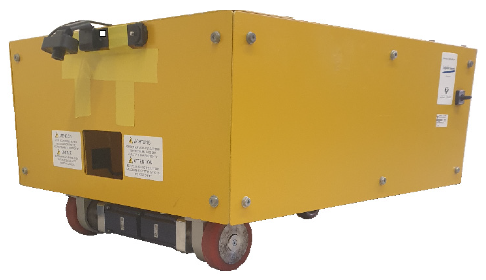
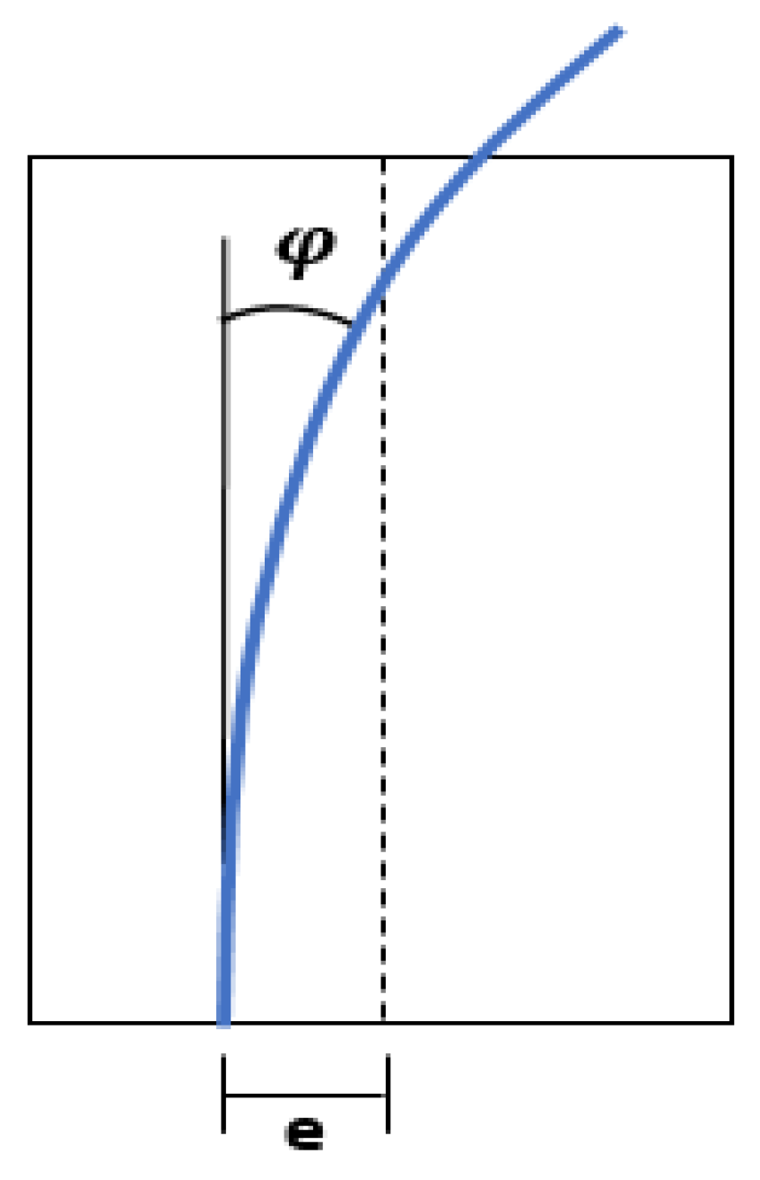
The fundamental objective of the present study is to ensure the stability of an indoor navigation algorithm in a 2D environment for the AGV shown in Figure 1. Based on Stanley’s algorithm, a lateral control adapted to this autonomous vehicle is proposed. The algorithm calculates the velocity and rotation angle commands to perform the movement, applying different mathematical operations. In this manner, lateral control and longitudinal control should coexist.

The main goal of the current work is to implement the algorithm in the AGV and be able to perform collision-free navigation. This issue is achieved by using computer vision and a neural network that segments the environment to generate a path.

2. Materials and Methods

This article presents an algorithm for indoor navigation of AGVs and the study of its stability. With the idea of the Stanley algorithm (see Hoffmann et al. [45]), this work proposes a modification because of the use of the AGV shown in Figure 1. This autonomous vehicle allows the adjustment of the angular and linear velocity criteria.

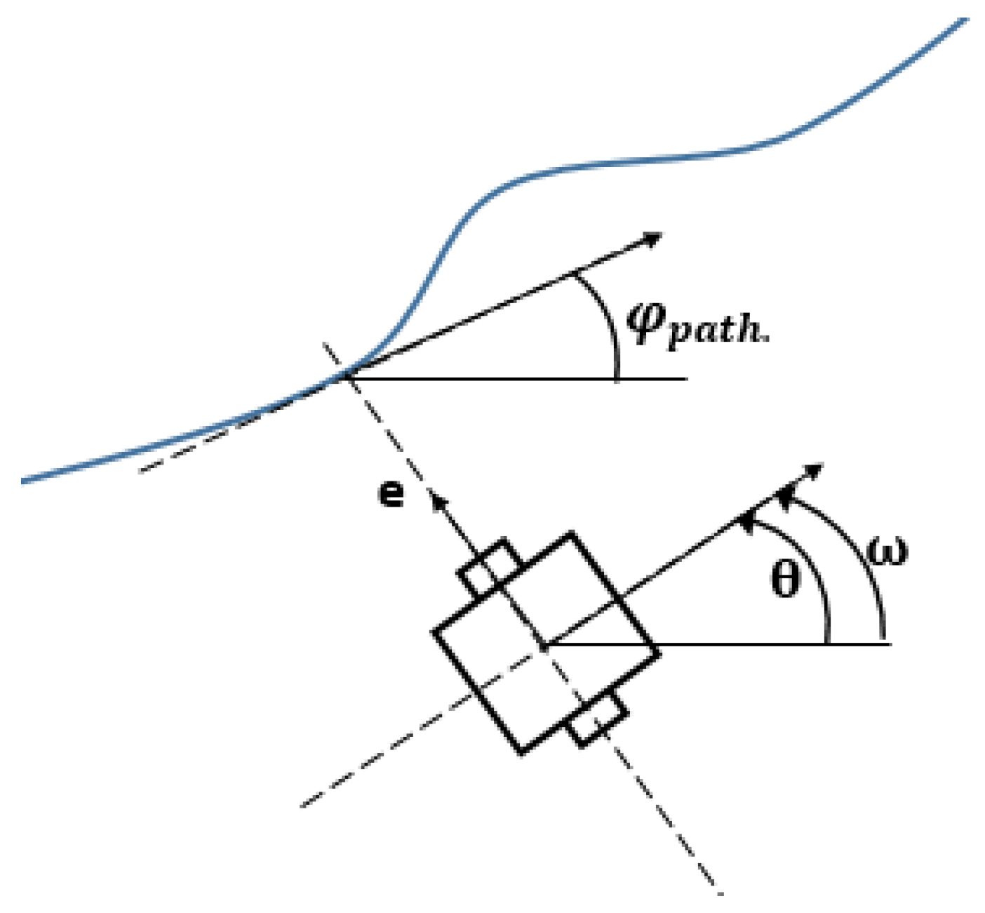
Accordingly, in this paper, the algorithm focuses on the lateral control of the AGV, acting mainly on the rotational speed $\dot{\theta }$ (rad/s). It is necessary to observe that the alignment error φ (rad) remains the difference between the vehicle angle $\theta$ (rad) and the path curvature φ_path (rad). The positioning error noted as e (m), refers to the minimum distance between the autonomous vehicle and the closest point of the trajectory in reference to the vehicle as represented in Figure 2.

The side wheels of the AGV used, rotate on the same axis, as represented in Figure 2. Note that ω should take into account both the positioning error noted as e and the alignment error noted as φ. The alignment error remains a revealed fact, so the positioning error is the variable, where two opposite cases are assumed. If e is remarkably large, it is of interest to situate the AGV perpendicular to the path, in order to get closer to it, so the value of φ is be $\frac{\pi }{2}$. In the case that e is significantly smaller, there is no alignment error, so it is of interest to keep both angles with the same value. The curve given by the values of φ is an Arctangent function, which also appears in Stanley’s algorithm.

In this manner, it is proposed to implement Stanley’s algorithm as shown in the following equations. Knowing that θ is derivable in time, the value that ω should have is proposed in Equation (1).

$$\frac{d\theta }{dt}=\omega =K_1({\phi }_{\mathrm{setpoint}}\left(e\right)-\left(\theta -{\phi }_{\mathrm{path}}\right)$$

(1)

The introduction of the parameter φ_setpoint (rad) is necessary, to adapt the range of values of φ. Its value is defined in Equation (2):

$${\phi }_{setpoint}\left(e\right)=arctg\left(K_2·e\right)$$

(2)

In this way, it is proposed to have two functions depending on the constants K₁ (s⁻¹) and K₂ (1/m), which are to be determined. It can be appreciated that the constant K₁ is the one related to the alignment error φ and K₂ controls the value of the positioning error e.

Some other equations also need to be accounted for. $\dot{x}$ (m/s) and $\dot{y}$ (m/s) represent the linear velocities in the directions of the axes, as indicated in Equations (3) and (4).

$$\dot{x}=V\cos \theta$$

(3)

$$\dot{y}=V\sin \theta$$

(4)

As mentioned throughout this work, the objectives of the lateral control are that the positioning error tends to be 0 and that θ equals φ_path.

A study is required to demonstrate the proposed design is stable for all types of paths. For this purpose, the Lyapunov function will be used. Through the study, it is equally possible to dictate the value of the constants K₁ and K₂ in Equations (1) and (2). The Lyapunov energy equation noted as L (m²) is proposed based on the previous equations in Equation (5).

$$\{\begin{array}{c}L=e^2>0\\ \frac{dL}{dt}<0\end{array}$$

(5)

For the first approach, the linear velocity V (m/s) is assumed to be constant.

The autonomous vehicle is placed with a random $\overrightarrow{pose}=\left[x, y, \theta \right]$ value, and the constants K₁ and K₂ are applied to the lateral control, analysing how the AGV behaves as a function of these coefficients. To simplify the analysis, a trajectory of the form Ax + By + C = 0 will be considered.

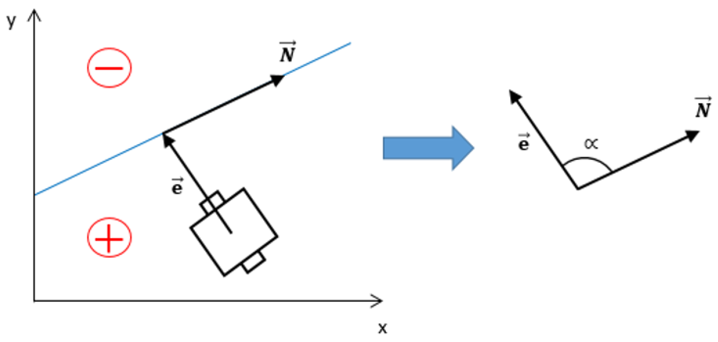
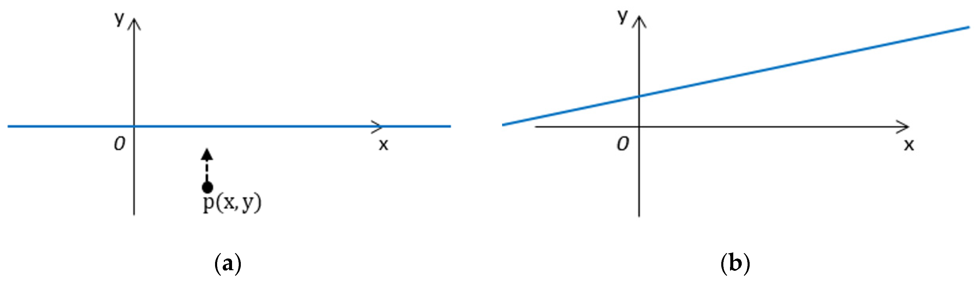
Distinction of the Positioning Error Sign

To implement the lateral control design, it is necessary to contemplate the sign of e because it is not taken into account in either of Equation (1) or Equation (2). It is necessary to differentiate on which side of the path the AGV is located because depending on this; it must be steered with a positive or negative sign.

Hence, to consider the sign, the positioning error e is to be taken as a vector $\overrightarrow{\mathrm{e}}$. The vector $\overrightarrow{\mathrm{N}}$ is the one that represents in which direction the AGV will follow the path. Finally, α is the angle formed between these two vectors, as illustrated in Figure 3.

Figure 3 also shows in which region the positioning error is considered positive and in which negative. Due to that consideration, the direction of $\overrightarrow{\mathrm{e}}$ is conditioned by that sign, representing the course the AGV needs to take to reduce the positioning error. Like so, if the AGV is on the right side of the path, the value of φ needs to be increased. If the AGV is on the left side, the value of the alignment error has to be reduced, supporting negative values. To resolve it, the vector product of $\overrightarrow{\mathrm{e}}$ and $\overrightarrow{\mathrm{N}}$ must be performed.

If $\left|\overrightarrow{N}\right| \mathrm{and} \left|\overrightarrow{e}\right|$ take the value 1, an analysis can be performed as a function of α. In case α is positive, the positioning error has to be positive as well. In the opposite case, that is when α is negative, the positioning error has to bear a negative sign. Knowing the path is defined, it is possible to acquire the values of the points P1(x, y) and P2(x, y).

P1 refers to the point on the path most adjacent to the AGV. The position of the autonomous vehicle is noted as p(x, y). In the case of P2, it refers to the nearest next point from the AGV after P1. Thus, the values of the vectors $\overrightarrow{e}$ and $\overrightarrow{N}$ can be determined as presented in Equations (6) and (7).

$$\overrightarrow{N}=\frac{\overrightarrow{P2}-\overrightarrow{P1}}{\Vert \overrightarrow{P2}-\overrightarrow{P1}\Vert }$$

(6)

$$\overrightarrow{e}=\overrightarrow{P1}-\overrightarrow{p}$$

(7)

With this knowledge, in the line of code that calculates the positioning error, it is necessary to apply the approximation of Equation (8) to consider the sign of e.

$$e \mathit{sin}\propto =T=N\left(1\right)e\left(2\right)-N\left(2\right)e\left(1\right)$$

(8)

Considering the path form and the previous equations, the positioning error is defined in Equation (9).

$$e=\frac{\left|Ax+By+C\right|}{\sqrt{A^2+B^2}}=\left(sign\left(e\right)\right)distmin.\left(\overrightarrow{p},path\right)$$

(9)

3. Proposal Explanation

A combination of neural networks and hardware devices, such as the AGV itself, is employed. Regarding the hardware, the use of a Beckhoff PLC (C6925) and its automation software allows the drivers to be managed on a real-time industrial platform. This platform is highly robust and widely used therein type of industrial applications. In addition, the employment of Matlab R2019b provides the advantage of utilizing a platform that allows very rapid development of control engineering algorithms. From a sensor point of view, and in the present case, the use of a vision-based navigation system that recognises lanes, the advantage resides in the fact that it is a very rapid way of implementing path-following systems.

3.1. Necessary Data Acquisition

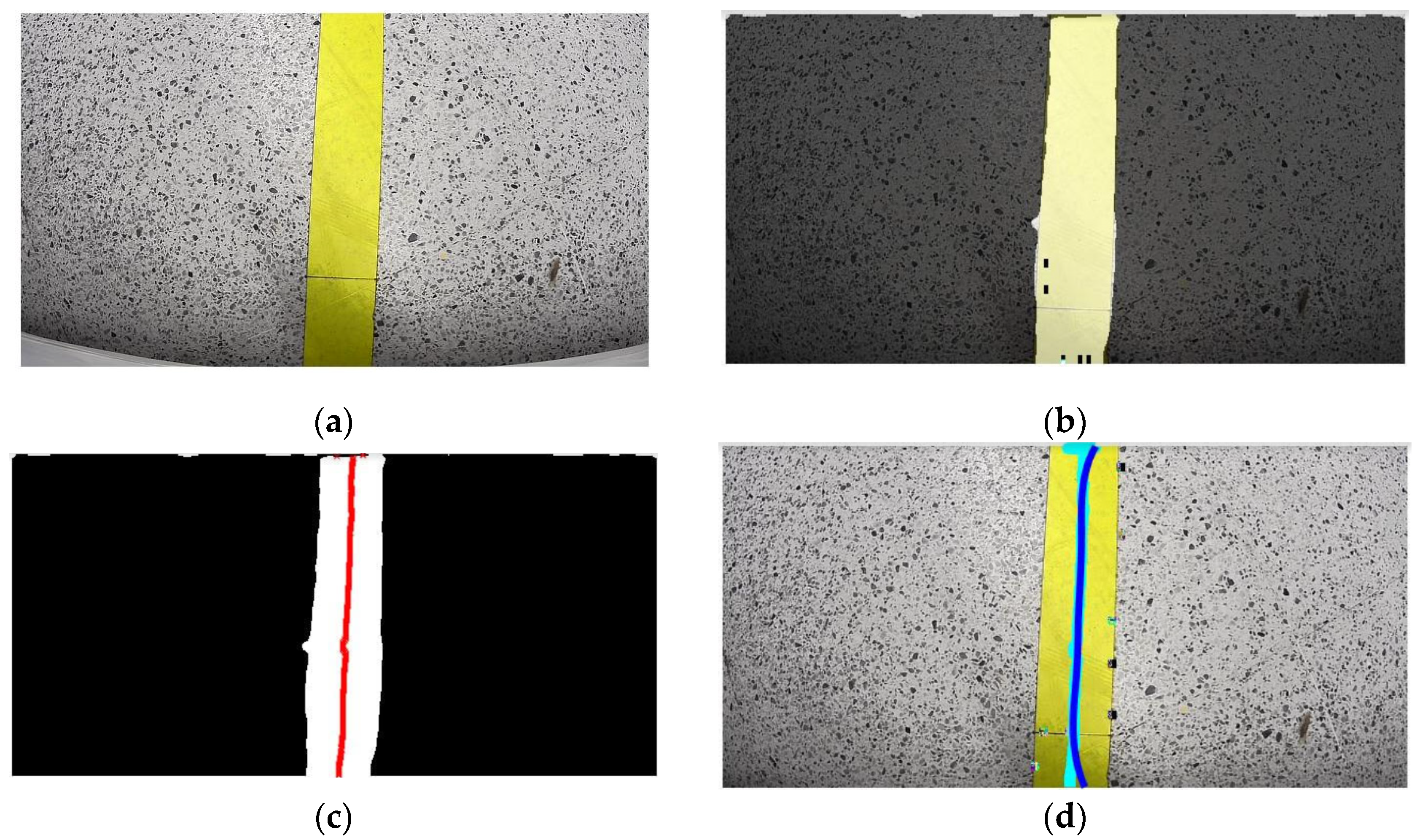
To obtain the trajectory, the example of the study by Teso-Fz-Betoño et al. [42] is followed. A convolutional neural network (CNN) is managed to perform semantic segmentation of an image. It is classified into several masks, generating a vector of the interest points from the mask corresponding to the navigation area. This vector with the position of the path in pixels x and y represents the information provided to the navigation algorithm. The scenario comprises a room with a yellow line representing the trajectory. The neural network has to detect this line, which will be followed by the AGV. This is concluded by employing a camera. The processing of the image is represented in Figure 4.

Figure 4a shows the image captured by the AGV, with the yellow line to be followed. After obtaining the image, the convolutional neural network performs semantic segmentation, obtaining two independent masks. The shaded mask constitutes the part that is not of interest to the autonomous vehicle, so the shinier one attends the important one, as illustrated in Figure 4b. In addition, the image is cropped at the lower part to remove the portion of the AGV that is captured by the camera.

From the clearest mask, the midpoints represented by red crosses are gained, as shown in Figure 4c. Thus, the trajectory to be followed by the AGV is obtained. Conclusively, the points approached with the semantic segmentation are connected to forge the path as represented in light blue in Figure 4d. Due to the pronounced curves generated in this path, an interpolation is performed to acquire a smoother trajectory, coloured with dark blue. The AGV follows that final trajectory.

With the image taken of the path, the AGV can acquire the information of the positioning error and the angle of the trajectory as graphed in Figure 5. Note that the measurement is produced considering the location of the AGV as the position of the camera. The camera is placed at the leading centre of the autonomous vehicle.

This approach provides all the data necessary for the navigation resolution.

3.2. Concurrency in the Approach

The designed algorithm has fast dynamics. This implies that regardless of the initial position of the AGV as a function of e, it is necessary to obtain an θ_optimun (rad) for the autonomous vehicle. This value is not the same as θ, and this is where K₁ comes in. θ_optimun refers to the sum between φ_path and φ_setpoint(e). Accordingly, because of the fast dynamic, the AGV orients itself on the way of the trajectory rapidly, being able to consider that the path has no inclination. This is depicted in Figure 6. In the case of the positioning error, it is not possible to make an approximation, and the path will be considered to be angled. In conclusion, it can be declared that the time constants of the orientation loop are smaller than those of the displacement. Ergo, two situations are envisaged as represented in Figure 6a,b.

With this approach, it is possible to analyse the stability of the system and to get the K₁ and K₂ values.

4. Value of K₁

4.1. System Stability Study

Lyapunov stability analysis is performed as mentioned above. Conventional techniques, for instance “frecuency” methods, are generally carried out on cases where the dynamical model of the system is linear. In the present study, the dynamical model is non-linear and the use of Lyapunov provides a generalist manner of assuring the stability of a dynamical system.

The first scenario is where can be assumed that the angle of the trajectory is zero, as illustrated in Figure 6a. Considering that assumption, the terms A and C of the path equation disappear, the path being By = 0. Hence, the study is simplified.

The initial consideration is when the AGV is away from the trajectory, so the positioning error value is obtained directly as indicated in Equation (10).

$$e=-y$$

(10)

The objective is to guarantee that the system is stable, being L consistently positive. Therefore, considering the previous equation, it can be formulated in Equation (11).

$$L=e^2=y^2$$

(11)

As the value of y is squared, it is confirmed that L is always positive, so the difficulty now lies in the second expression of Equation (5). In this manner, the derivate must be considered taking into account the Equation (12).

$$\frac{dL}{dt}=2·e·\dot{e}=2·y·\dot{y}$$

(12)

Additionally, Equation (1) can be restated considering φ_path = 0, as shown in Equation (13).

$$\dot{\theta }=K_1\left({\phi }_{setpoint}\left(e\right)-\theta \right)$$

(13)

As mentioned, assuming that the dynamic of Equation (13) is extremely fast, it is possible to obtain the value of the angle θ, because of the rapid tendency of the AGV will have, positioning with the orientation of Figure 6a. Then θ is defined in Equation (14).

$$\theta ={\phi }_{setpoint}\left(e\right)=arctg\left(K_2·e\right)$$

(14)

Equation (4) can directly be raised anew, bearing in mind Equations (10) and (14).

$$\dot{y}=V\sin \left(-arctg\left(K_2·y\right)\right)=-V\sin \left(arctg\left(K_2·y\right)\right)$$

(15)

To obtain the value of $\dot{L}$, the Equation (12) can be complemented with that seen in Equation (15).

$$\dot{L}=2y\left(-V\sin \left(arctg\left(K_2·y\right)\right)\right)$$

(16)

By the way, Equation (2) is designed knowing that K₂ will always be positive, so the following remarks can be made.

$$sign\left(arctg\left(K_2·y\right) \right)=sign\left(y\right)$$

(17)

$$sign\left(\sin \left(arctg\left(K_2·y\right)\right)\right)=sign\left(arctg\left(K_2·y\right)\right)$$

(18)

This leads to the following conclusion.

$$sign\left(y\right)=sign\left(\sin \left(arctg\left(K_2·y\right)\right)\right)$$

(19)

With this information, analysing Equation (19) and knowing the positioning error is negative as stated in Equation (10), it can be guaranteed that the Lyapunov function is fulfilled.

4.2. Procurement of Value of K₁

For the system to be stable when the AGV is distant from the trajectory, it has been assumed that the dynamics are so fast. Accordingly, the AGV is oriented perpendicular to the path. In addition, it will approach rapidly, producing a minor positioning error, which is considered to be zero. Carrying on with that consideration, therein case, only the angle of the AGV can be taken into account, reformulating Equation (13).

$$\dot{\theta }=K_1\left(0-\theta \right)=-K_1\theta$$

(20)

In this situation, it is necessary to study again the stability of the system. Recalling the Lyapunov system of Equations (11) and (12), it will not be a problem to confirm that L is by squaring. The problem is again in the derivative of the energy. The study examines the case where the AGV is under the trajectory, so it is recognized that in that area θ will allow positive values. So, if e is null, it is also comprehensible that θ tends to be equal to φ_path. Therefore, one can formulate the integral of Equation (20), which remains a linear system.

$$\theta =\frac{\pi }{2}ex{p}^{-K_1·\tau }$$

(21)

Equation (12) requires the value of y and $\dot{y}$, which can be obtained from Equation (4) by substituting Equation (21).

$$\dot{y}=V\sin \left(\frac{\pi }{2}ex{p}^{-K_1\tau }\right)$$

(22)

$$y=V{{\displaystyle \int }}_0^t\sin \left(\frac{\pi }{2}ex{p}^{-K_1\tau } \right)d\tau +y\left(0\right)$$

(23)

From Equation (22) it can be deduced that the value is always negative because the function sin is always between 0 and π. In the case of Equation (23), the initial condition is also always negative, so it is necessary to ensure that the integral never obtains a value greater than y(0), to confirm the stability. So it is necessary to guarantee that the positioning error never changes sing, whereby the value of K₁ can be known. In Equations (24) and (25) the integral is noted as I.

$$y=VI\left(K_1, t\right)+y\left(0\right)<0$$

(24)

$$VI\left(K_1,t\right)<-y\left(0\right)$$

(25)

Thus, the linear velocity and K₁ are related. Analysing Equations (23) and (25), the following conclusions can be drawn. If the value of K₁ is very aggressive, the exponential tends to 0 quickly obtaining a sinusoidal function with value 0 and making the expression vanish very briefly. This makes it independent of the value V that is set. On the contrary, if K₁ is small, the velocity is limited. Otherwise, an undesired oscillation system would appear.

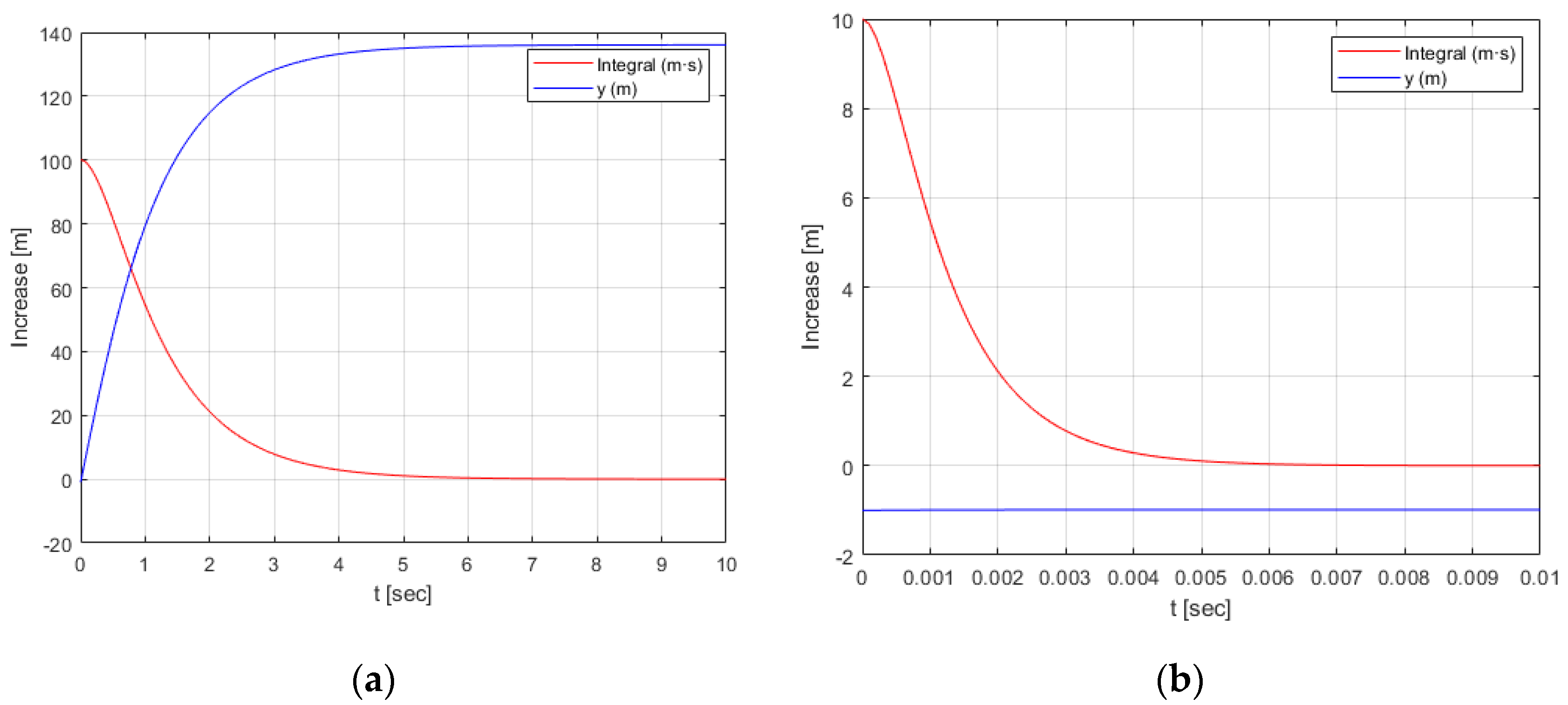
This system is implemented in Matlab Ver. R2019b (The Matworks Inc., Madrid, Spain), obtaining the plots revealed in Figure 7. In Figure 7a the values of V = 100 m/s and K₁ = 1 s⁻¹ are set for plotting. It can be visualized how the value of the integral (red line) takes time to fade out, in the order of seconds. In this case, the value of y admits an extremely significant positive value which does not ensure stability as it cannot be guaranteed to be lower than y(0). In the plot of Figure 7b, V = 10 m/s and K₁ = 1000 s⁻¹ are set. The value of the integral disappears instantly, ensuring the stability of the system and regardless of the velocity value set.

With this analysis, the need for longitudinal control is acknowledged to ensure that the system is always stable. As 10 m/s is a reasonable speed value for the AGV used, the value of K₁ is set to 1000 s⁻¹. This value refers to the gain of the alignment error control loop.

5. Value of K₂

5.1. System Stability Study

As previously indicated in the stability analysis of the K₁ value, once again a non-linear system is observed, so Lyapunov is employed in order to ensure stability.

The second scenario to be investigated is when the angle of the trajectory needs to be taken into account, as shown in Figure 6b. As already known, the system has highly fast dynamics so Equation (1) is adapted because the AGV assumes the desired direction very quickly. As K₁ is already defined, it can be ignored.

$$\dot{\theta }={\phi }_{setpoint}\left(e\right)+{\phi }_{path}\left(e\right)$$

(26)

Therein situation, φ_path must also attend a function that depends on the positioning error, due to the position (x, y) of the AGV. Depending on this, the most adjacent point of the path will vary. In this case, the positioning error is calculated as in Equations (27) and (28).

$$\left(x_{near},y_{near}\right)=Argmin(\Vert \left(x,y\right)-\left(x_{path},y_{path}\right)\Vert )$$

(27)

$${\phi }_{path}\left(e\right)= {\phi }_{path}\left(x_{near},y_{near}\right)$$

(28)

Resolving this analytically can be complex. Remembering the Lyapunov system of Equation (5), the e can be defined as in Equation (9). However, this time it is necessary to calculate the parameters A, B and C, considering the position of the AGV because the sign of e depends on that.

$$\{\left(A, B, C\right)=f\left(\left(x_{near},y_{near}\right),\overrightarrow{p}\right)$$

(29)

Due to the added difficulty, the systems must be expounded in a discrete form. An optimization algorithm is proposed in which e is calculated for every point in a bounded area. With this information and fixing θ, K₂ is varied, allowing its value to be dictated. The following system is considered at instant t.

$$\theta \left(x,y,K_2\right)=f\left(e,K_2\right)+{\phi }_{path}\left(e\right)$$

(30)

$$e\left(x\left(t\right),y(t\right))=e\left(t\right)$$

(31)

Knowing that e and θ depend on the position of the AGV and K₂, it is possible to determine some expression at t + dt, taking into account Equations (3) and (4).

$$x\left(t+dt\right)=x+V\cos \theta$$

(32)

$$y\left(t+dt\right)=y+V\sin \theta$$

(33)

$$e\left(x\left(t+dt\right),y\left(t+dt\right)\right)=e\left(t+dt\right)$$

(34)

$$∆e=e\left(t+dt\right)-e\left(t\right)$$

(35)

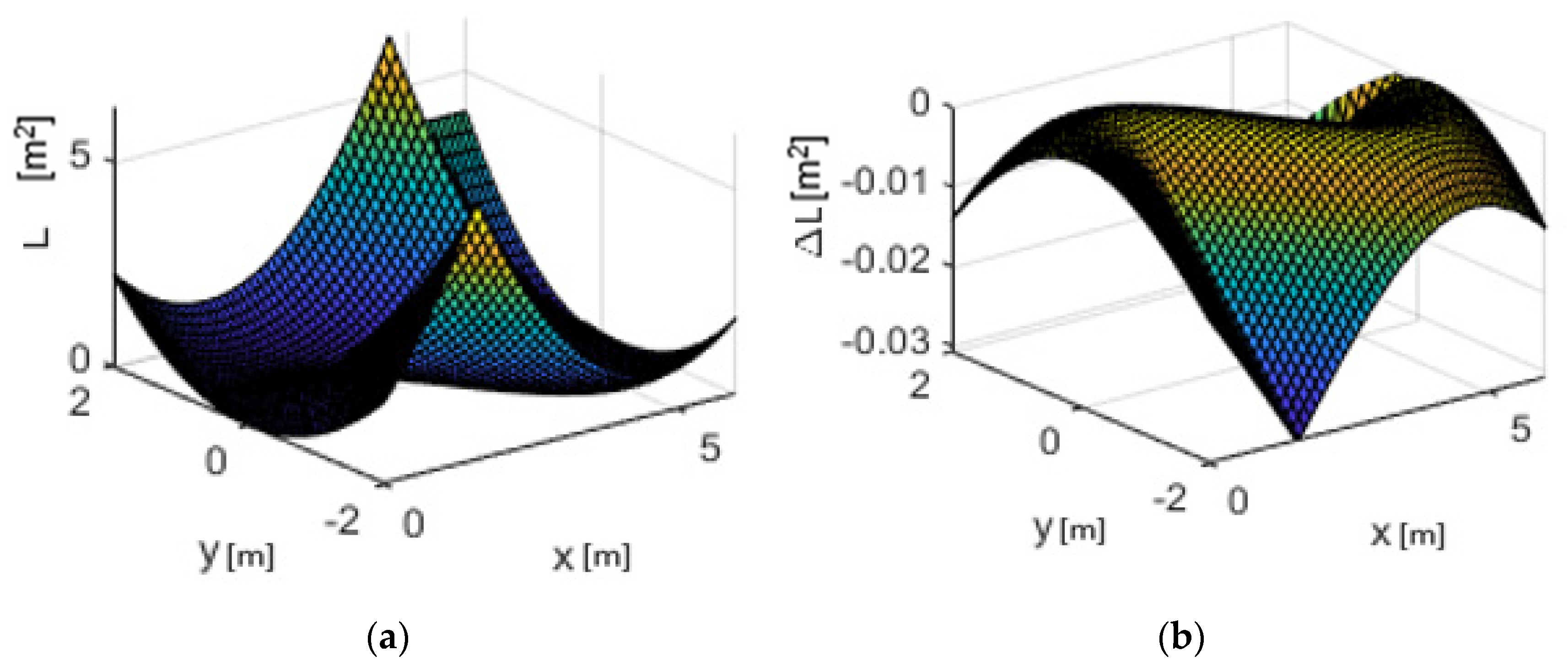
Equation (35) has to be negative to ensure stability. The problem is discontinuities can be generated. This issue occurs when the closest point of the path at t is not the same at t + dt or does not continue in the corresponding direction. Instead of considering the whole e (from AGV to the path), it is analysed in sections, guaranteeing that Equation (35) is negative. Hence, the value of Δe is to be taken in absolute values to demonstrate the system is stable. A simulation is performed on all $\overrightarrow{p}$ of a bounded area to visualize this phenomenon. It is affected by a sinusoidal trajectory as it is more in line with reality (curves and straight lines).

Figure 8a shows that the Lyapunov energy function is consistently positive over the whole space. L represents a (m²) value. The derivative of L in Figure 8b is negative throughout the space considered, coinciding with the value of the variation of the positioning error. Therefore, the stability of the system is confirmed.

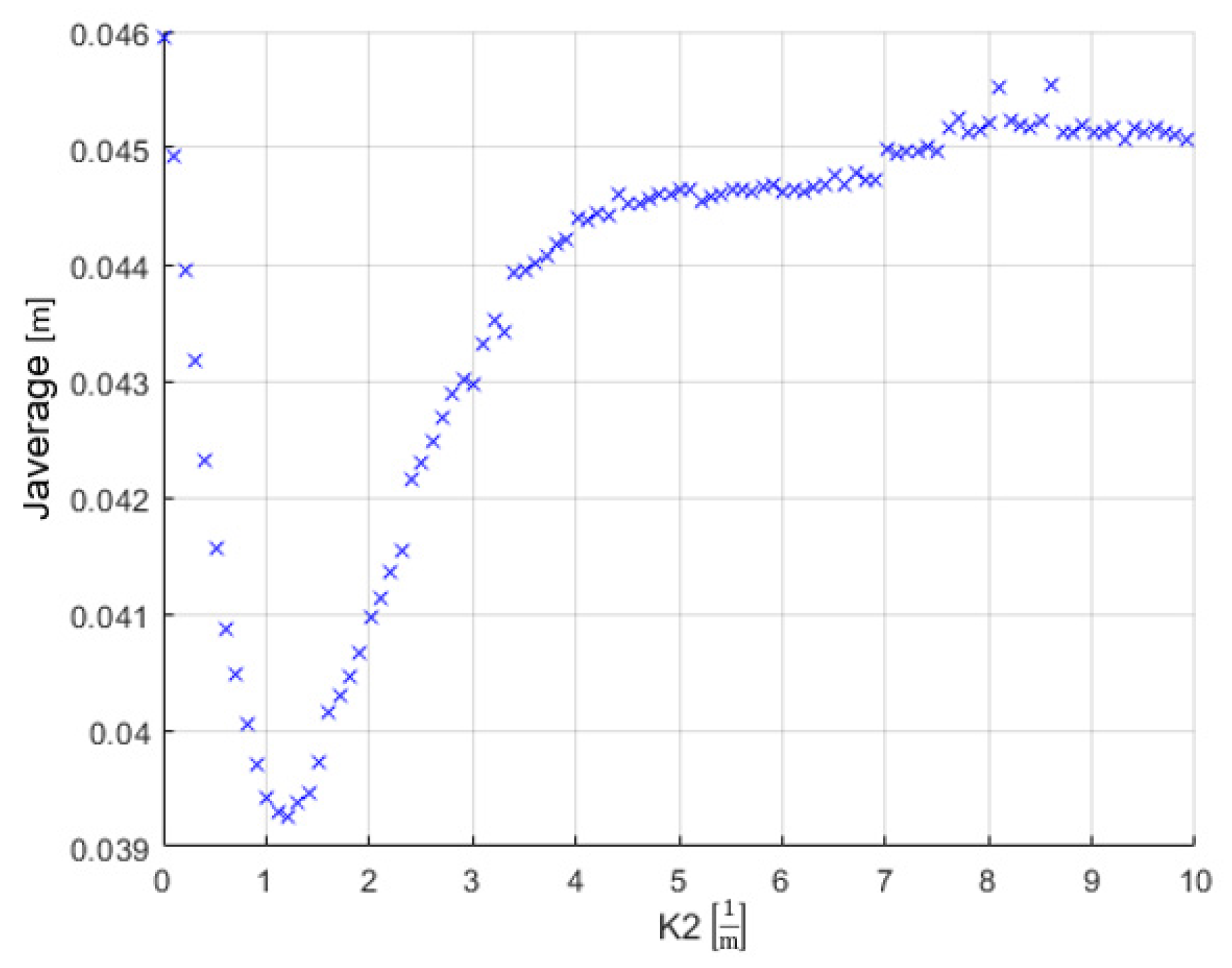
5.2. Optimization of Value of K₂

Once it is comprehended that the system is stable, a code has been generated that tests all the values of K₂ in a range for the whole amount $\overrightarrow{p}$. By setting a value of K₂ it is possible to visualize the evolution of Δe, and the optimal value can be acquired. In Equations (36) and (37), a cost function is proposed that depends on the mean square error, denoted as J.

$$\parallel e\parallel =\sqrt{{\left(x-x_{near}\right)}^2+{\left(y-y_{near}\right)}^2}$$

(36)

$$J=\frac{1}{t}\left({{\displaystyle \int }}_0^t\parallel e\left(K_2,\overrightarrow{p}, path\right)\parallel dt\right)=\frac{1}{N}{\displaystyle \sum }_{k=0}^{k=N}{e}^2\left(k\right)$$

(37)

This provides the average of J, as a function of the initial position of the AGV.

$$E_{\overrightarrow{p}}\left(K_2,\overrightarrow{p}, path\right)=\overline{J}\left(K_2,\overrightarrow{p}, path\right)$$

(38)

The path persists in attending to a non-variable parameter, just like $\overrightarrow{p}$, so to vary J the entirely dependent value is K₂, formulated in Equation (39).

$$K_2=Argmin\left(\overline{J}\right)$$

(39)

The optimization strategy in this test is to perform an exhaustive analysis of all possible combinations of the space in order to get the most optimal result. This approach is simulated, resulting in the K₂ values presented in Figure 9.

This figure also shows that there is an optimal value that minimizes J. Note that K₂ attends the parameter that acts on the rate of evolution of the φ_setpoint. Accordingly, this value is set as K₂ = 1.21 (1/m).

6. Longitudinal Control Algorithm

As already noted, the trajectory represents an acknowledged fact, so it is possible to identify the state of a point at t + 1. It is equally recognized that there are curves in the path so each point must provide a tangential acceleration, denoted as a_T (m/s²) and a normal acceleration, denoted as a_N (m/s²). The latter can be defined as in Equation (40), from which $\rho$ (m) can be known.

$$a_N=\frac{V^2}{\rho }={\omega }^2\rho =V\omega$$

(40)

In the same way, it is decided that a_N needs to be under maximum speeding up, called a_Nmax (m/s²), as in Equation (41).

$$\parallel a_N\parallel \le a_{Nmax}$$

(41)

Due to Equation (41), it is possible to achieve the linear velocity from Equation (40).

$$V=\frac{a_N}{\omega }$$

(42)

Keep in mind that the angular velocity is given by K₁ and K₂, so a maximum velocity can be fixed as well, as in Equation (43).

$${V_{max}}^{\prime }=\frac{a_{Nmax}}{\omega }$$

(43)

Therefore, by taking Equation (43) it is possible to enhance the value of the linear velocity of the AGV, allowing it to be determined by the positioning error.

$$V=\min \left(\frac{a_{Nmax}}{\omega }, V_{max}=f\left(e\right)\right)$$

(44)

Equation (44) contemplates the velocity policy designed in a previous section. Depending on e the AGV adjusts the speed, but it will also be subject to the curvature of the trajectory. It is substantial to know the angle that the path will occupy at the continuous instant, being able to predict the V at t + 1. In that manner, the AGV will have knowledge of if it is close to a curve, allowing it to reduce the velocity. Therefore, with this idea of prediction, the vectors that compose the acceleration are proposed, perceiving the relation of Equation (45), where a represents the acceleration (m/s²).

$$a^2=a_N{}^2+a_T{}^2\to a_T=\sqrt{a^2-a_N{}^2}$$

(45)

With this information, it is possible to propose the velocity at t + 1 for the AGV.

$$V\left(t+1\right)=V\left(t\right)+∆t·a_T$$

(46)

In Equation (46) it is viable to substitute a_T, as seen in Equation (40).

$$V\left(t+1\right)=V\left(t\right)+∆t\sqrt{a^2-V{\left(t\right)}^2\omega {\left(t\right)}^2}$$

(47)

Knowing all the variables of Equation (47), it is possible to obtain the value of the maximum speed at t + 1, denoted as V_max″. Taking into account Equation (44), Equation (48) is defined.

$$V\left(t+1\right)=\min \left({V_{max}}^{″}, {V_{max}}^{\prime }=f\left(e\right)\right)$$

(48)

To such a degree, if the AGV maintains a significantly high angular velocity, the linear speed is reduced. The parameter V_max′ is provided by the AGV, representing the maximum nominal velocity.

$$V\left(t+1\right)=f\left(e, \omega \left(t\right),V\left(t\right), a\right)$$

(49)

Ultimately, e is contemplated, attaching importance to the trajectory execution speed.

7. Results

Beforehand, the algorithm is proved in simulation, analysing the compliance drop the various objectives. As designed, the lateral control and the longitudinal control work together to allow proper trajectory tracking. In the simulations, it is observed that regardless of the values of the $\overrightarrow{pose}$, the autonomous vehicle redirects and reaches the path. As the AGV approaches, it adjusts itself to be able to develop over the trajectory and not overshoot it, obtaining correct trajectory tracking.

At the beginning of the simulation, the algorithm can determine the closest position of the trajectory based on the AGV. Therefore, the first objective is to attain that point. In this situation, the value of the positioning error is considerable. Regardless of the initial θ, the AGV is required to take an angle of $\frac{\pi }{2}$ (rad) to correct the value of e and reach the trajectory quickly. When the AGV assumes θ =$\frac{\pi }{2}$ rad, the forward motion begins. With the decrease in the positioning error, the value of the vehicle angle starts adapting, adjusting to fit the trajectory angle and generating a curve. The linear velocity also starts increasing. As the AGV approaches the path, the closest point is necessarily unmaintained.

While the positioning error decreases, the alignment error has to do so as well. Because of that, and as the closest point is changing, the value of φ is adapting.

When the AGV is on a straight trajectory, both error values are approximately null, making accurate tracking of the trajectory achievable. In this case, the speed of the movement is limited by the V_nom of the AGV. In the case of a curve in the path, it can be observed that the autonomous vehicle reduces its speed to prevent deviating from the predetermined path. Simultaneously, it is making a constant redirection to adhere to the reduced value of alignment error.

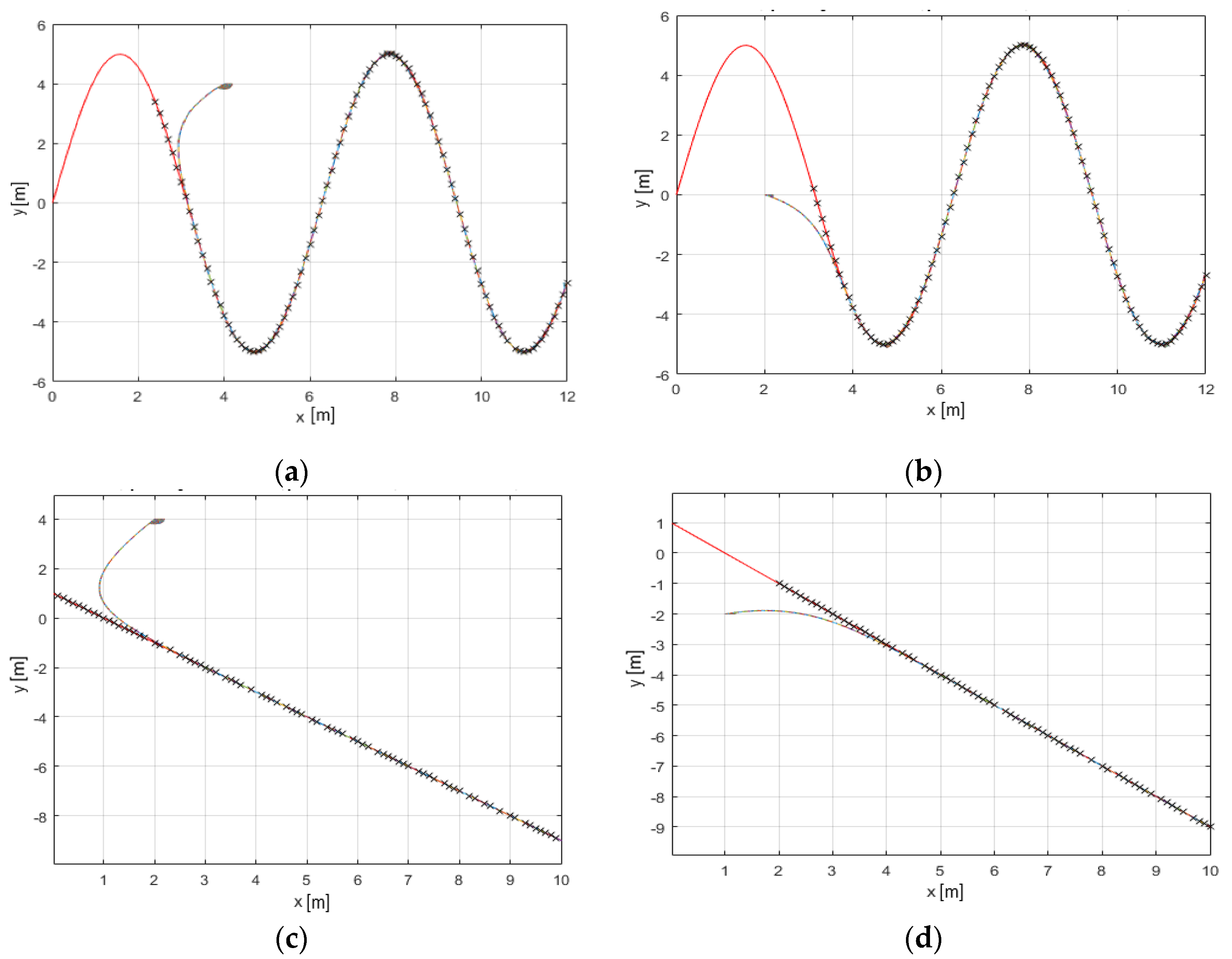
In this way, it is proved that the designed algorithm produces a satisfactory result due to the good following of any type of trajectory as can be seen in Figure 10. It exhibits diverse types of paths and $\overrightarrow{pose}$s of the AGV. The red line represents the established trajectory. The black crosses are the nearest point calculated by the algorithm. The coloured line represents the route followed by the AGV. It can be perceived that irrespective of the positioning error, the navigation algorithm performs well in all cases. In Figure 10a,b, the established path is sinusoidal where it can be seen how the AGV can reach the trajectory and adapt to it in both cases. In Figure 10c,d a purely linear trajectory is considered where the AGV also tracks the path well. At long last, a fully curved trajectory is presented in Figure 10e,f. Once more, the following is performed accurately.

Additionally, it can be marked from all the graphs in Figure 10 that the tracking of the trajectory is correct independently of the positioning of the AGV and therefore, of the sign of e.

It is equally necessary to test whether the algorithm as a whole is suitable for the real AGV. To perform this, two instances are created in MATLAB. One of them processes the image, and the other one executes the navigation algorithm. These are communicated by ROS nodes, to give concurrency to the execution. The movement of the AGV is achieved with a PLC. It is observed that the AGV can follow the whole route correctly.

In the interest of clarifying the execution times of the algorithm, it should be marked that the processor employed is Intel^® Core™ i9-9880H CPU @ 2.30 GHz 3.30 GHz. The RAM memory of the computer on which the algorithm is executed is 16 GB and it has an NVIDIA Quadro T1000 graphics card.

Under these conditions, the neural network execution time is 144ms. This time is incorporated into the total period of the ROS publishing node, which is the one that manages the images and takes 186 ms to send the trajectory data vector, measured as an average of 1550 executions.

Regarding the subscriber node, that is the one that executes the control and sends the commands to the PLC, it takes 136 ms on average in 5510 iterations.

8. Discussion

In considering the advantages of this study, comparisons with other techniques commonly used in the control of AGVs are mentioned.

On the one hand, one of the most frequently used sensor techniques in this type of vehicles is LiDAR. These devices are highly effective when it comes to localizing ad receiving data related to the environment in which the AGV is located. In studies such as the one performed by Quan and Chen [46], these devices are employed in conjunction with the odometry of the wheels in order to localize an autonomous guided vehicle. Despite their extensive use, these sensors do not provide the necessary robustness for this type of systems. In the present paper, this robustness is consistently achieved.

On the other hand, in the industrial field, it has been frequent to employ philo-guided vehicles (see Chet et al. [47]). These vehicles use electromagnetism to perform navigation, providing the necessary robustness and accuracy. However, it is not a flexible solution. The AGV and navigation system presented in this work have the benefit of achieving minimum cost when implementing a fixed trajectory. By the use of tape of a determined color, any type of path can be established without the need for expensive and specific infrastructure. Furthermore, with the re-training of the neural network the path can be adapted to any color or operating area.

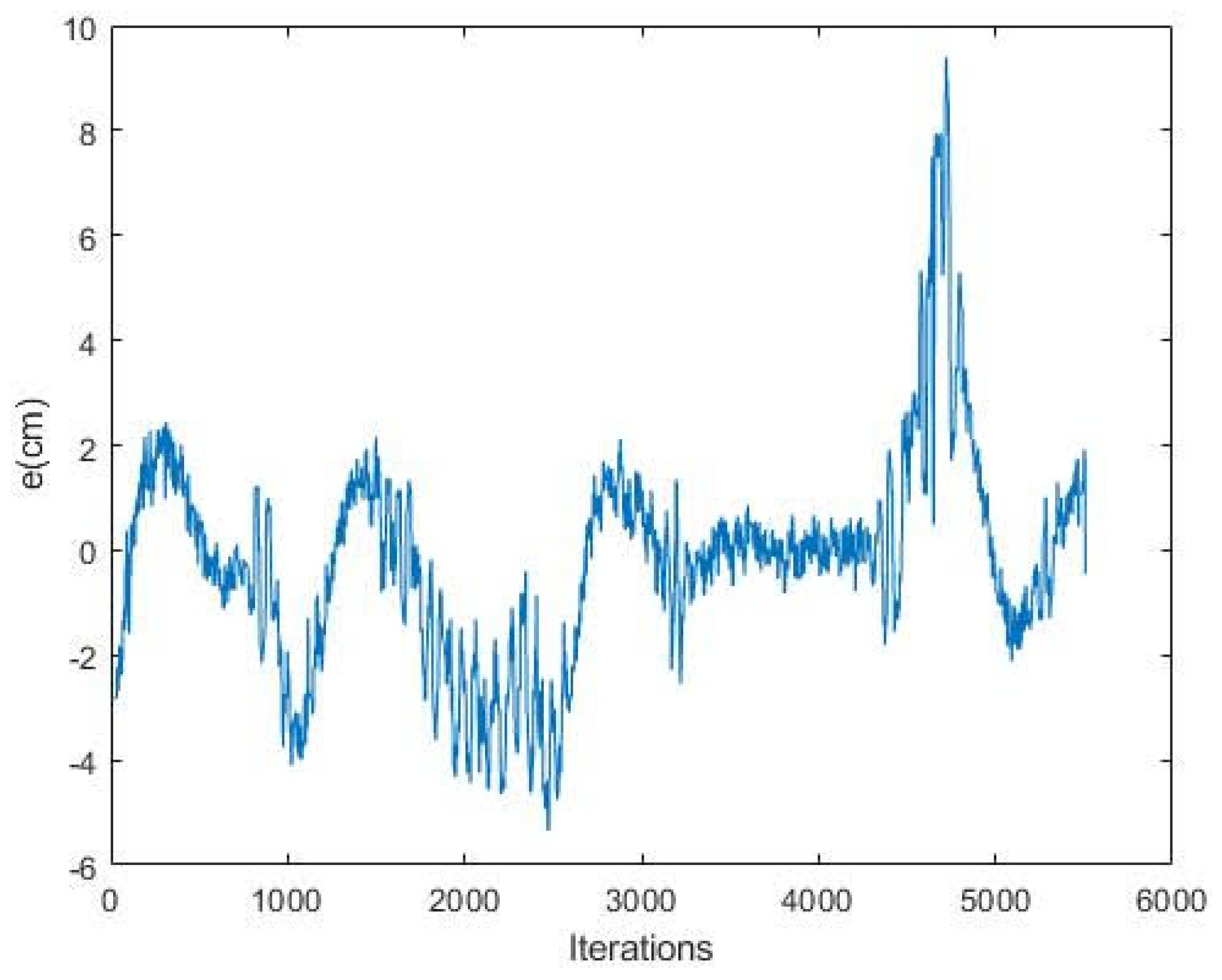
To conclude, it is possible to get the positioning error committed with this navigation algorithm in a specific trajectory, as graphited in Figure 11. The figure, therefore, shows that in curved areas, like in the beginning and the end iterations, the positioning error increases, because of the location of the wheels and the camera in the AGV itself. However, in the central iterations, it can be appreciated that in straight areas the positioning error is close to zero.

As demonstrated by Hoffmann et al. [45] in the Stanley algorithm, a typical RMS cross-track error of less than 0.1 m is obtained. In the case of this modification of the algorithm, the RMS of the positioning error is around 0.02 m.

9. Conclusions

The present work focuses on the search for solutions for the navigation and localization of an AGV, because of the need to discover robust techniques, achieving greater precision and reliability.

Fundamentally, it is demonstrated that the proposed algorithm modification is stable. As mentioned in the previous section, the advantages over conventional techniques can be recognized. This algorithm is remarkably simple, requiring no previous training to perform properly. When changing path, no retraining is necessary, it merely requires the colour of the trajectory to match.

In terms of navigation, starting from a base such as the Stanley algorithm and presenting it another perspective comprehends its complexity. In addition, demonstrating stability and ensuring the given solution is adequate is uneasy. For this, other alternatives have to be tested until a solution is obtained that proves its robustness. Therein way, the values of the constants can be demonstrated and a sense for them, as well. This issue has been one of the most arduous tasks of this work.

The main objective set in this work represents the stability analysis of the modification of a navigation algorithm capable of performing lateral control and longitudinal control. This has been achieved, obtaining satisfactory results. As mentioned, the difficulty was in the stability analysis, but due to the results, its proper performance has been demonstrated.

Continuing with localization, instead of designing a new algorithm, some data derived from the other algorithms are employed. In this case, the necessary parameters can be obtained from the navigation and path planning codes, without using sensors.

Sensors remain the conventional method for calculating the trajectory. In this work, it is completed with artificial vision and a neural network, a less common method but with remarkably pleasing results as well. The latter algorithm was considered with Hough transforms, for example, but concluded that the use of a neural network was more appropriate. Nevertheless, in some areas, further study is required to achieve more accuracy. These areas are related to light shimmers generated in the image that create indistinctness.

Furthermore, it has been possible to decouple the problem of data acquisition from the problem of navigation. Consequently, until a new image is received, predictions are used.

Overall, the work accomplishes the objective of ensuring stability of an algorithm for the free navigation of an industrial autonomous vehicle.

As a prolongation of this research, attempts will be made to enhance the architecture of the convolutional neural network with the aim of achieving higher speed rates.

For future work, the execution of the algorithm in real-time but with more excessive speed may reveal a lack in the concurrency of the ROS nodes. An analysis of resource consumption can in addition be effected.

On the other hand, numerous tests can be done with the neural network, changing the configuration or performing different learning, to improve the accuracy of the navigable path. This can give an idea of the characteristics that the CNN may need for this application.

An explicability analysis using the LIME technique can clarify whether the semantic segmentation errors are related to the similarities between the images. In all images, the trajectory is mostly linear and close to the centre of the image. This analysis provides insight into what the neural network relies on to classify the parts of the image. It will also be interesting to investigate the interpretation of deep learning.

In addition, if the semantic segmentation has mask discontinuities to compute the trajectory, it is necessary to consider alternatives in the algorithm to finalize the navigation.

As for the algorithm used, it is necessary to incorporate the case where there is no trajectory and how to stop the AGV’s movement. In the simulation, the AGV attains the final of the trajectory and turns π (rad), following the path in reverse. In the real AGV, when it does not visualize any more trajectory, it starts to turn on its own to detect the yellow line again. Therefore, there exists an understandable need for a stopping policy that contemplates different situations.