XCM: An Explainable Convolutional Neural Network for Multivariate Time Series Classification

Abstract

Multivariate Time Series (MTS) classification has gained importance over the past decade with the increase in the number of temporal datasets in multiple domains. The current state-of-the-art MTS classifier is a heavyweight deep learning approach, which outperforms the second-best MTS classifier only on large datasets. Moreover, this deep learning approach cannot provide faithful explanations as it relies on post hoc model-agnostic explainability methods, which could prevent its use in numerous applications. In this paper, we present XCM, an eXplainable Convolutional neural network for MTS classification. XCM is a new compact convolutional neural network which extracts information relative to the observed variables and time directly from the input data. Thus, XCM architecture enables a good generalization ability on both large and small datasets, while allowing the full exploitation of a faithful post hoc model-specific explainability method (Gradient-weighted Class Activation Mapping) by precisely identifying the observed variables and timestamps of the input data that are important for predictions. We first show that XCM outperforms the state-of-the-art MTS classifiers on both the large and small public UEA datasets. Then, we illustrate how XCM reconciles performance and explainability on a synthetic dataset and show that XCM enables a more precise identification of the regions of the input data that are important for predictions compared to the current deep learning MTS classifier also providing faithful explainability. Finally, we present how XCM can outperform the current most accurate state-of-the-art algorithm on a real-world application while enhancing explainability by providing faithful and more informative explanations.

1. Introduction

Following the remarkable availability of multivariate temporal data, Multivariate Time Series (MTS) analysis is becoming a necessary procedure in a wide range of application domains (e.g., finance [1], healthcare [2], mobility [3], and natural disasters [4]). A time series is a sequence of real values ordered according to time; and when a set of coevolving time series are recorded simultaneously by a set of sensors, it is called an MTS. In this paper, we address the issue of MTS classification, which consists of learning the relationship between an MTS and its label.

According to the results published, the most accurate state-of-the-art MTS classifier on average is a deep learning approach (MLSTM-FCN [5]). MLSTM-FCN consists of the concatenation of a Long Short-Term Memory (LSTM) block with a Convolutional Neural Network (CNN) block composed of three convolutional sub-blocks. However, MLSTM-FCN outperforms the second-best MTS classifier (Bag-of-Words method WEASEL+MUSE [6]) only on the large datasets (relatively to the public UEA archive [7]—training set size ≥ 500). This deep learning approach contains a significant number of trainable parameters, which could be an important reason for its poor performance on small datasets. Moreover, for many applications, the adoption of machine learning methods cannot rely solely on their prediction performance. For example, the European Union’s General Data Protection Regulation (GDPR), which became enforceable on 25 May 2018, introduces a right to explanation for all individuals so that they can obtain “meaningful explanations of the logic involved” when automated decision making has “legal effects” on individuals or similarly “significantly affecting” them (https://ec.europa.eu/info/law/law-topic/data-protection_en (accessed on 1 November 2021)). As far as we have seen, an architecture concatenating a LSTM network with a CNN such as MLSTM-FCN, or a classifier based on unigrams/bigrams extraction following a Symbolic Fourier Approximation [8] such as WEASEL+MUSE, cannot provide perfectly faithful explanations as they rely solely on post hoc model-agnostic explainability methods [9], which could prevent their use in numerous applications. Faithfulness is critical as it corresponds to the level of trust an end-user can have in the explanations of model predictions, i.e., the level of relatedness of the explanations to what the model actually computes. Hence, we propose a new compact (in terms of the number of parameters) and explainable deep learning approach for MTS classification that performs well on both large and small datasets while providing faithful explanations.

CNNs along with post hoc model-specific saliency methods such as Gradient-weighted Class Activation Mapping—Grad-CAM [10]—have the potential to have a compact architecture while enabling faithful explanations [11]. A recent CNN, MTEX-CNN [12] proposes using 2D and 1D convolution filters in sequence to extract key MTS information, i.e., information relative to the observed variables and time, respectively. However, as confirmed by our experiments, the features related to time which are extracted from the output features of the first stage (relative to each observed variable) cannot fully incorporate the timing information from the input data and subsequently yield poor performance compared to the state-of-the-art MTS classifiers. In addition, the significant number of trainable parameters of MTEX-CNN affects its generalization ability on small datasets. Finally, MTEX-CNN requires upsampling processes on feature maps when applying Grad-CAM, which can lead to an imprecise identification of the regions of the input data that are important for predictions.

Therefore, we propose a new faithfully eXplainable CNN method for MTS classification (XCM) which improves MTEX-CNN in three substantial ways: (i) it generates features by extracting information relative to the observed variables and timestamps in parallel and directly from the input data; (ii) it enhances the generalization ability by adopting a compact architecture (in terms of the number of parameters); and (iii) it allows precise identification of the observed variables and timestamps of the input data that are important for predictions by avoiding upsampling processes. Summarizing our main contributions:

• We present XCM, an end-to-end new compact and explainable convolutional neural network for MTS classification which supports its predictions with faithful explanations;
• We show that XCM outperforms the state-of-the-art MTS classifiers on both the large and small UEA datasets [7];
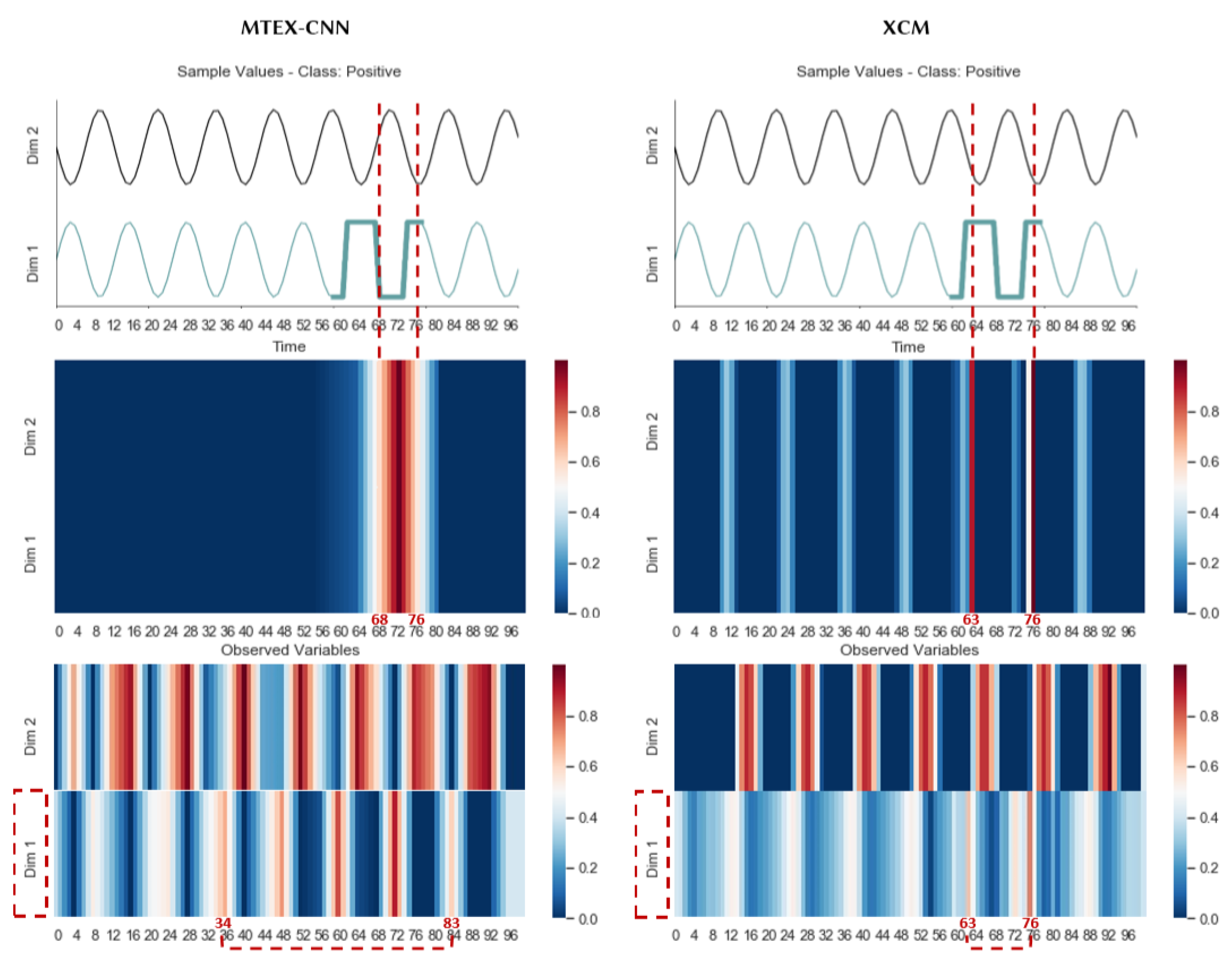
• We illustrate on a synthetic dataset that XCM enables a more precise identification of the regions of the input data that are important for predictions compared to the current faithfully explainable deep learning MTS classifier MTEX-CNN;
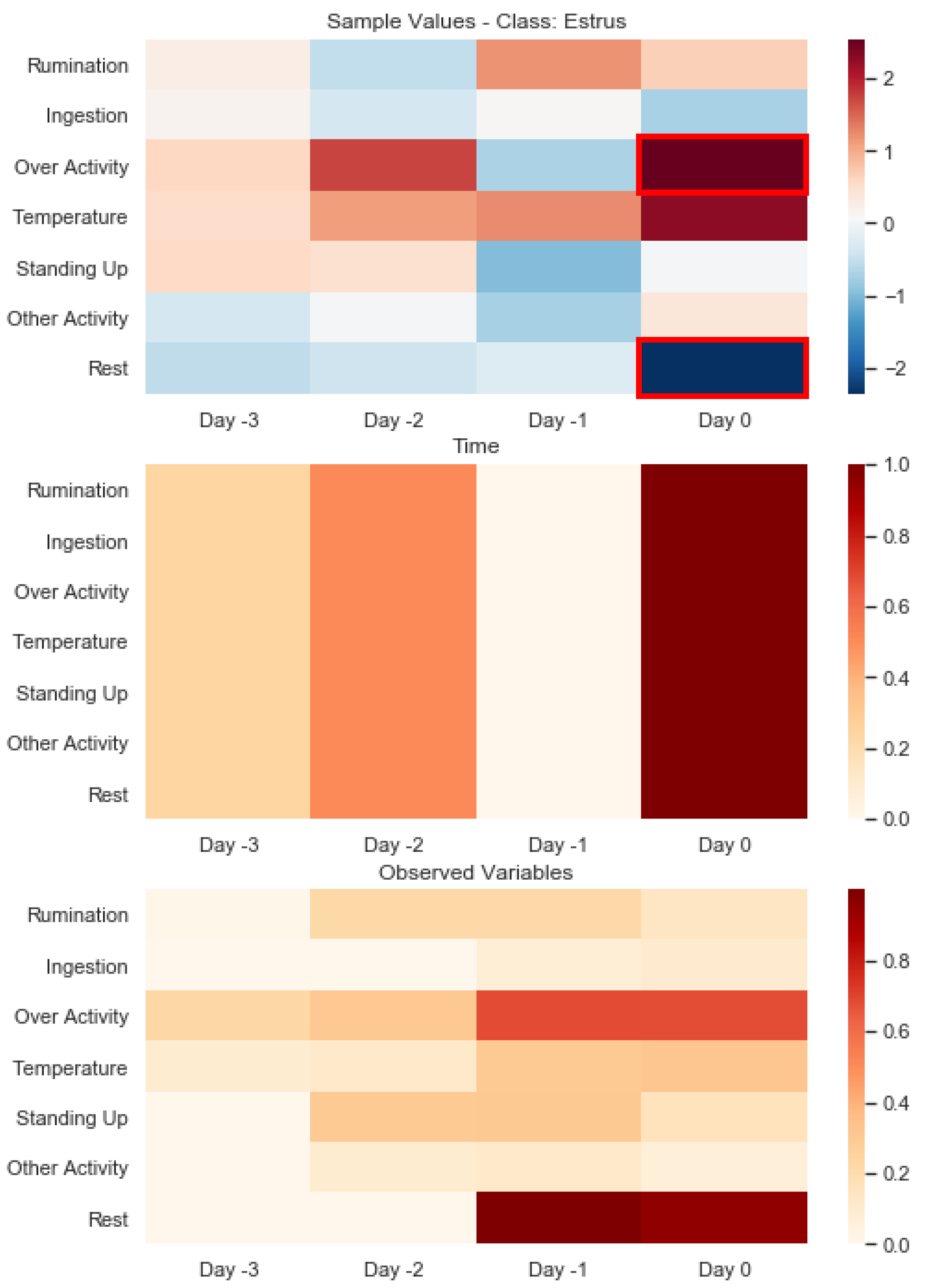
• We show that XCM outperforms the current most accurate state-of-the-art algorithm on a real-world application while enhancing explainability by providing faithful and more informative explanations.

The rest of this paper is organized as follows: Section 2 presents the related work concerning MTS classification and explainability; Section 3 details XCM architecture; Section 4 presents our evaluation method; and finally, Section 5 discusses our results.

2. Related Work

In this section, we first introduce the background of our study. Then, we present the state-of-the-art MTS classifiers, and we end with existing explainability methods supporting CNNs models’ predictions.

2.1. Background

We address the issue of supervised learning for classification. Classification consists of learning a function that maps an input data to its label: given an input space X, an output space Y, an unknown distribution P over $X\times Y$, a training set sampled from P, and a 0–1 loss function ${\ell }_{0-1}$ compute function $h^{*}$ as follows:

$$h^{*}=\underset{h}{argmin}{\mathbb{E}}_{(x,y)\sim P}\left[{\ell }_{0-1}(h,(x,y))\right]$$

(1)

In this study, classification is performed on multivariate time series datasets. A Multivariate Time Series (MTS) $M=\{x_1,\dots ,x_d\}\in {\mathcal{R}}^{d*l}$ is an ordered sequence of $d\in \mathcal{N}$ streams with $x_i=(x_{i,1},\dots ,x_{i,l})$, where l is the length of the time series and d is the number of multivariate dimensions. We address MTS generated from automatic sensors with a fixed and synchronized sampling along all dimensions. An example of an MTS with two dimensions and a length of 100 is given at Section 5.

Before presenting the state-of-the-art MTS classifiers, we introduce some notions about neural networks and the subfamily of our approach, Convolutional Neural Networks (CNNs). A neural network is a composition of L parametric functions referred to as layers, where each layer is considered a representation of the input domain [13]. One layer $l_i$, such as $i\in \{1,\dots ,L\}$, contains neurons, which are small units that compute one element of the layer’s output. The layer $l_i$ takes as input the output of its previous layer $l_{i-1}$ and applies a transformation to compute its own output. The behavior of these transformations is controlled by a set of parameters ${\theta }_i$ for each layer and an activation sublayer to shape the nonlinearity of the network. These parameters are called weights and link the input of the previous layer to the output of the current layer based on matrix multiplication. This process is also referred to as feedforward propagation in the deep learning literature and is the constituent of multilayer perceptrons (MLPs). A neural network is usually called “deep” when it contains more than one layer between its input and output layer. Following the good performance of CNN architectures in image recognition [14] and natural language processing [15,16], CNNs have started to be adopted for time series analysis [17]. CNNs are neural networks that use convolution in place of general matrix multiplication in at least one of their layers [13]. A convolution can be seen as applying and sliding a filter over the time series. The use of different types, numbers and sequences of filters allow the learning of multiple discriminative features (feature maps) useful for the classification task.

2.2. MTS Classifiers

The state-of-the-art MTS classifiers are usually grouped into three categories: similarity-based, feature-based and deep learning methods.

Similarity-based methods make use of similarity measures to compare two MTS (e.g., Euclidean distance). Dynamic Time Warping (DTW) has been shown to be the best similarity measure to use along with the k-Nearest Neighbors (k-NN) [18]. DTW is not a distance metric as it does not fully satisfy the required properties (the triangle inequality in particular), but its use as similarity measure along with the NN-rule is valid [19]. There are two versions of kNN-DTW for MTS, dependent (DTW${}_D$) and independent (DTW${}_I$), and neither dominates the other [20]. DTW${}_I$ measures the cumulative distances of all dimensions independently measured under DTW. DTW${}_D$ uses a similar calculation with single-dimensional time series; it considers the squared Euclidean accumulated distance over the multiple dimensions.

Next, feature-based methods can be categorized into two families: shapelet-based and Bag-of-Words (BoW) classifiers. Shapelets models (gRSF [21] and UFS [22]) use subsequences (shapelets) to transform the original time series into a lower-dimensional space that is easier to classify. On the other hand, BoW models (LPS [23], mv-ARF [24], SMTS [25] and WEASEL+MUSE [6]) convert time series into a bag of discrete words and use a histogram of words representation to perform the classification. WEASEL+MUSE shows better results compared to gRSF, LPS, mv-ARF, SMTS and UFS on average (20 MTS datasets). WEASEL+MUSE generates a BoW representation by applying various sliding windows with different sizes on each discretized dimension (Symbolic Fourier Approximation) to capture features (unigrams, bigrams and dimension identification). Following a feature selection with chi-square test, it classifies the MTS based on a logistic regression.

Finally, deep learning methods (FCN [26], MLSTM-FCN [5], MTEX-CNN [12], ResNet [27], TapNet [28] and TST [29]) use Long-Short Term Memory (LSTM), Convolutional Neural Networks (CNN) or Transformers. According to the results published and our experiments, the current state-of-the-art model (MLSTM-FCN) is proposed in [5] and consists of a LSTM layer and a stacked CNN layer along with squeeze-and-excitation blocks to generate latent features. A recent network, TapNet [28], also consists of a LSTM layer and a stacked CNN layer, followed by an attentional prototype network. However, TapNet shows lower accuracy results (https://github.com/xuczhang/xuczhang.github.io/blob/master/papers/aaai20_tapnet_full.pdf (accessed on 1 November 2021)) on average on the 30 public UEA MTS datasets compared to MLSTM-FCN (MLSTM-FCN results presented in Table 3). There is no basis of comparison for MLSTM-FCN with MTEX-CNN [12] as MTEX-CNN has not been evaluated on public datasets. As illustrated in Section 3, MTEX-CNN is a two-stage CNN network which first extracts information relative to each feature with 2D convolution filters and then extracts information relative to time with 1D convolution filters. The output feature map is fed into fully connected layers for classification.

Therefore, in this work, we choose to benchmark XCM to the best-in-class for each similarity-based, feature-based and deep learning category (DTW${}_D$/DTW${}_I$, WEASEL+ MUSE and MLSTM-FCN classifiers). We also include MTEX-CNN in the benchmark to demonstrate the superiority of our approach as MTEX-CNN has not been evaluated on the public UEA datasets.

2.3. Explainability

In addition to their prediction performance, machine learning methods have to be assessed on how they can support their decisions with explanations. Two levels of explanations are generally distinguished: global and local [30]. Global explainability means that explanations concern the overall behavior of the model across the full dataset, while local explainability informs the user about a particular prediction. As previously introduced with the example of the GDPR, our new CNN approach needs to be able to support each individual prediction. Thus, we present in this section the local explainability methods for CNNs.

CNNs classifiers do not provide explainability-by-design at the local level. Thus, some post hoc model-agnostic explainability methods could be used. These methods provide explanations for any machine learning model. They treat the model as a black-box and do not inspect internal model parameters. The main line of work consists of approximating the decision surface of a model using an explainable one (e.g., LIME [31], SHAP [32], Anchors [33] and LORE [34]). However, the explanations from the surrogate models cannot be perfectly faithful with respect to the original model [9], which is a prerequisite for numerous applications.

Then, some post hoc model-specific explainability methods exist. These methods are specifically designed to extract explanations for a particular model. They usually derive explanations by examining internal model structures and parameters. The approaches based on back-propagation are seen as the state-of-the-art explainability methods for deep learning models [35]. Methods based on back-propagation (e.g., Gradient Explanation [36], Guided Backpropagation [37], $\epsilon$-Layer-wise Relevance Propagation [38], Gradient ⊙ Input [39], Integrated Gradients [40], DeepLift [41] and Grad-CAM [10]) calculate the gradient, or its variants, of a particular output with respect to the input using back-propagation to derive the contribution of features. In particular, Gradient-weighted Class Activation Mapping (Grad-CAM) [10] has proven to be an adequate method for supporting CNNs predictions. Grad-CAM identifies the regions of the input data that are important for predictions in CNNs using the class-specific gradient information. The method has been shown to provide faithful explanations with regard to the model [11]. The faithfulness of the explanations provided by Grad-CAM is shown following a methodology based on model parameter and data randomization tests. However, the precision of the explanations provided by Grad-CAM, i.e., the fraction of explanations that are relevant to a prediction, can vary across CNN architectures as Grad-CAM is sensitive to the upsampling processes on feature maps to match the input data dimensions.

Therefore, we support the predictions of our new CNN model XCM with Grad-CAM, a post hoc model-specific explainability method which provides faithful explanations at local level. The design of our network architecture avoids upsampling processes and enables Grad-CAM to identify the observed variables and timestamps of the input data that are important for predictions more precisely as compared to what the current explainable deep learning MTS classifier MTEX-CNN give.

Table 1. Overview of the state-of-the-art MTS classifiers.

	ED	DTW	MLSTM FCN	MTEX CNN	WEASEL+ MUSE	XCM
Performance
Small Datasets					✓	✓
Large Datasets			✓			✓
Explainability
Faithful Explainability	✓	✓		✓		✓

presents an overview of the challenges addressed by the state-of-the-art MTS classifiers and how we position our new method XCM. We evaluate the classification performance of XCM and its explainability in Section 5. The next section presents XCM in details.

3. XCM

In this section, we present our new eXplainable Convolutional neural network for Multivariate time series classification (XCM). The first part details the architecture of the network, and the second part explains how XCM can provide explanations by identifying the observed variables and timestamps of the input data that are important for predictions.

3.1. Architecture

Our approach aims to design a new compact and explainable CNN architecture that performs well on both the large and small UEA datasets. As illustrated in Figure 1, a recent explainable CNN, MTEX-CNN [12], proposes to use 2D and 1D convolution filters in sequence to extract key MTS information, i.e., information relative to the observed variables and time, respectively. However, CNN architectures such as MTEX-CNN have significant limitations. The use of 2D and 1D convolution filters in sequence means that the features related to time (features maps from 1D convolution filters) are extracted from the processed features related to observed variables (features maps from 2D convolution filters). Therefore, features related to time cannot fully incorporate the timing information from the input data and can only partially reflect the necessary information to discriminate between the different classes. Thus, (i) our approach XCM extracts both features related to observed variables (2D convolution filters) and time (1D convolution filters) directly from the input data, which leads to more discriminative features by incorporating all the relevant information and ultimately to a better classification performance on average than the 2D/1D sequential approach (see results in Section 5.1). Then, a CNN architecture using fully connected layers to perform classification, especially with the size of the first layer depending on the time series length as in MTEX-CNN, is prone to overfitting and can lead to the explosion of the number of trainable parameters. Thus, (ii) the output feature maps of XCM are processed with a 1D global average pooling before being input to a softmax layer for classification. The use of 1D global average pooling followed by a softmax layer for classification reduces the number of parameters and improves the generalization ability of the network compared to fully connected layers. Global average pooling consists of summarizing each feature map by its average. This operation improves the generalization ability of the network, as it does not have parameters to train, and it provides robustness to spatial translations of the input [42]. In the possible cases when the sequences of events in an MTS change, the robustness to spatial translation ensures that the classification result is not modified. Finally, the use of non fully padded convolution filters as in MTEX-CNN can lead to an imprecise identification of the regions of the input data that are important for predictions as Grad-CAM is sensitive to upsampling processes. Therefore, (iii) the 2D and 1D convolution filters of XCM are fully padded. As detailed in the next section, the output feature maps can then be analyzed with the Grad-CAM explainability method without altering the precision of the explanations through upsampling processes. Figure 2 illustrates XCM, and the following paragraphs detail the architecture.

Firstly, XCM extracts information relative to the observed variables with 2D convolution filters (upper green part in Figure 2). This upper part is composed of one 2D convolutional block which is then converted to one feature map to reduce the number of parameters with a $1\times 1$ convolution filter. The convolutional block contains a 2D convolution layer followed by a batch normalization layer [43] and a ReLU activation layer [44]. We set the kernel size of the 2D convolution filters to $WindowSize\times 1$, where $WindowSize$ is a hyperparameter which specifies the time window size, i.e., the size of the subsequence of the MTS expected to be interesting to extract discriminative features, and $\times 1$ means for each observed variable. Thus, these 2D convolution filters (number: F in Figure 2) allow the extraction of features per observed variable. The features are extracted using a sliding window (strides equal to 1), and we use padding instead of half padding to keep the dimension of the feature maps the same as the input data. The padding allows us to avoid using upsampling and interpolation methods on the features maps when building the attribution maps, i.e., the heatmaps of dimensions $T\times D$ that identify the regions of the input data that are important for predictions (detailed in the next section). Then, batch normalization brings normalization at the layer level, and it enables faster convergence and better generalization of the network [45]. In addition, the ReLU activation layer induces nonlinearity in the network. Next, the output feature maps are fed into a module ($1\times 1$ convolution filter) [46] which reduces the number of parameters. It projects the feature maps into one following a channel-wise pooling.

In parallel, XCM extracts information relative to time with 1D convolution filters (lower red part in Figure 2). This lower part is the same as the upper part, except that the 2D convolution filters are replaced by 1D. We set the kernel size of the 1D convolution filters to $WindowSize\times D$, where $WindowSize$ is the same hyperparameter as 2D convolution filters and D is the number of observed variables of the input data. The 1D convolution filters slide over the time axis only (stride equals to 1) and capture the interaction between the different time series. Following the use of padding, the output feature map of this lower part has a dimension of $T\times 1$, with T the time series length of the input data. The use of padding, similar to 2D convolution filters, allows us to avoid using upsampling of the features maps on the dimension related to the information extracted (time-T) when building the attribution maps (detailed in the next section).

In the following step, the output feature maps from these two parts are concatenated and form a feature map of dimensions $T\times (D+1)$. We apply the same 1D convolution block (1D convolution layer—F filters, kernel size $WindowSize\times (D+1)$, stride 1 and padding + batch normalization + ReLU activation layer) as presented in the previous paragraph to slide over the time axis and capture the interaction between the features extracted. Finally, we add a 1D global average pooling on the output feature maps and perform classification with a softmax layer. As previously introduced, the use of global average pooling instead of fully connected layers improves the generalization ability of the network.

In order to assess the potential advantage of concatenating the 2D and 1D convolution blocks instead of having them in sequence, independently from the choice of the classification layers (fully connected layers as in MTEX-CNN versus 1D global average pooling with a softmax layer in XCM), we include in our experiments in Section 5.1, a variant of XCM (XCM-Seq). XCM-seq is the same as XCM except that the 2D and 1D convolution blocks are in sequence. The next section presents how the architecture of XCM allows the communication of explanations supporting the model predictions with Grad-CAM.

3.2. Explainability

The new CNN architecture of XCM has been designed to enable the precise identification of the observed variables and timestamps that are important for predictions based on Gradient-weighted Class Activation Mapping (Grad-CAM) [10]. As presented in Section 2.3, Grad-CAM identifies the regions of the input data that are important for predictions in CNNs using the class-specific gradient information. More specifically, Grad-CAM can output two types of attribution maps from XCM architecture: one related to observed variables and another one related to time. Attribution maps are heatmaps of the same size as the input data where some colors indicate features that contribute positively to the activation of the target output [35]. These attribution maps constitute the explanations provided to support XCM model predictions and are available at the sample level. The following paragraphs explain how we adapt Grad-CAM for XCM.

In order to build the first attribution map related to observed variables, Grad-CAM is applied to the output feature maps of the 2D convolution layer which uses convolution filters per observed variable (first block in the upper green part in Figure 2). To obtain the class-discriminative attribution map, $L_{2D}^c\in {\mathbb{R}}^{T\times D}$ with T the time series length and D the number of observed variables, we first compute the gradient of the score for class c ($y_c$) with respect to feature map activations $A^k$ of the convolutional layer, i.e., $\frac{\partial y_c}{\partial A^k}$ with $k\in [1,\dots ,F]$ the identifier of the feature map. These gradients flowing back are global-average-pooled over the time series length (T) and observed variables (D) dimensions (indexed by i and j, respectively) to obtain the weight of each feature map. Thus, as regards the feature map k, we calculate the weight as:

$$w_k^c=\frac{1}{T\times D}\sum _i\sum _j\frac{\partial y_c}{\partial A_{ij}^k}$$

(2)

We then use the weights to compute a weighted combination between all the feature maps for that particular class and use a ReLU to keep only the positive attributions to the predictions (Equation (3)).

$$L_{2D}^c=ReLU\left(\sum _k{w}_k^c{A}^k\right)$$

(3)

The second attribution map, $L_{1D}^c$, relates to time and is built on the same principle. Grad-CAM is applied to the output feature maps of the 1D convolution layer which uses convolution filters sliding over the time axis (first block in the lower red part in Figure 2). With respect to the feature maps activations M and the class c, we calculate $L_{1D}^c$ as:

$$q_k^c=\frac{1}{T}\sum _i\frac{\partial y_c}{\partial M_i^k}$$

(4)

$$L_{1D}^c=ReLU\left(\sum _k{q}_k^c{M}^k\right)$$

(5)

Thus, $L_{1D}^c$ has $T\times 1$ as dimensions. We then upsample it to match the input data dimensions $T\times D$ with a bilinear interpolation in order to obtain the attribution map. This operation does not alter the time attribution results as the padding on the 1D convolution filters ensured that the feature extraction over the time dimension has kept the time series length. Therefore, the upsampling only replicates the results over the observed variables. An example of observed variables and time attribution maps on a synthetic dataset is presented in Section 5.2.

Before discussing the performance and explainability results of XCM, we present in the next section the evaluation setting.

4. Evaluation

In this section, we present the methodology employed (datasets, algorithms, hyperparameters and metrics) to evaluate our approach.

4.1. Datasets

We benchmarked XCM on the 30 currently available public UEA MTS datasets [7]. We kept the train/test splits provided in the archive. The characteristics of each dataset are presented in

Table 2. UEA MTS datasets. Abbreviations: AS—Audio Spectra, ECG—Electrocardiogram, EEG—Electroencephalogram, HAR—Human Activity Recognition and MEG—Magnetoencephalography.

Datasets	Type	Train	Test	Length	Dimensions	Classes
Articulary Word Recognition	Motion	275	300	144	9	25
Atrial Fibrilation	ECG	15	15	640	2	3
Basic Motions	HAR	40	40	100	6	4
Character Trajectories	Motion	1422	1436	182	3	20
Cricket	HAR	108	72	1197	6	12
Duck Duck Geese	AS	60	40	270	1345	5
Eigen Worms	Motion	128	131	17,984	6	5
Epilepsy	HAR	137	138	206	3	4
Ering	HAR	30	30	65	4	6
Ethanol Concentration	Other	261	263	1751	3	4
Face Detection	EEG/MEG	5890	3524	62	144	2
Finger Movements	EEG/MEG	316	100	50	28	2
Hand Movement Direction	EEG/MEG	320	147	400	10	4
Handwriting	HAR	150	850	152	3	26
Heartbeat	AS	204	205	405	61	2
Insect Wingbeat	AS	30,000	20,000	200	30	10
Japanese Vowels	AS	270	370	29	12	9
Libras	HAR	180	180	45	2	15
LSST	Other	2459	2466	36	6	14
Motor Imagery	EEG/MEG	278	100	3000	64	2
NATOPS	HAR	180	180	51	24	6
PenDigits	Motion	7494	3498	8	2	10
PEMS-SF	Other	267	173	144	963	7
Phoneme	AS	3315	3353	217	11	39
Racket Sports	HAR	151	152	30	6	4
Self Regulation SCP1	EEG/MEG	268	293	896	6	2
Self Regulation SCP2	EEG/MEG	200	180	1152	7	2
Spoken Arabic Digits	AS	6599	2199	93	13	10
Stand Walk Jump	ECG	12	15	2500	4	3
U Wave Gesture Library	HAR	120	320	315	3	8

.

4.2. Algorithms

We compare our algorithm XCM implemented in Python 3.6 (code available on GitHub https://github.com/XAIseries/XCM (accessed on 1 November 2021)) to the state-of-the-art MTS classifiers, as detailed in Section 2.2, and to the variant XCM-Seq:

• DTW${}_D$, DTW${}_I$ and ED—with and without normalization (n): we reported the results published in the UEA archive [7];
• MLSTM-FCN: we used the implementation available (https://github.com/houshd/MLSTM-FCN (accessed on 1 November 2021)) and ran it with the parameter settings recommended by the authors in the paper [5] (128-256-128 filters, kernel sizes 8/5/3, initialization of convolution kernels Uniform He, reduction ratio of 16, 250 training epochs, dropout of 0.8, Adam optimizer) and with the following hyperparameters: batch size $\{1,8,32\}$, number of LSTM cells $\{8,64,128\}$;
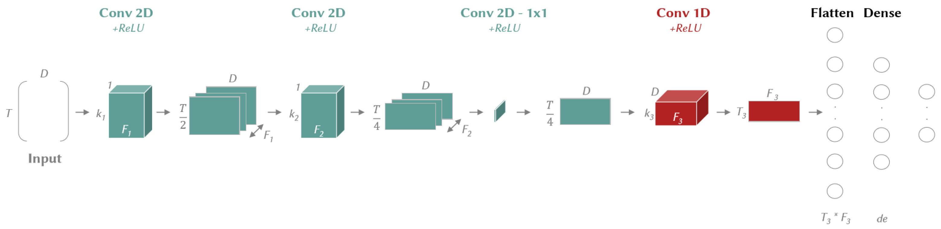
• MTEX-CNN: we implemented the algorithm with Keras in Python 3.6 based on the description of the paper [12]. We ran it with the parameter settings recommended by the authors (Stage 1: two convolution layers with half padding and ReLU activation, kernel sizes $8\times 1$ and $6\times 1$, strides $2\times 1$, feature maps 64 and 128, dropout 0.4. Stage 2: one convolution layer with ReLU activation, strides 2, kernel size 2, feature maps 128, dropout 0.4. Dense layer dimension 128 and L2 regularization 0.2) and with the following hyperparameter: batch size $\{1,8,32\}$;
• WEASEL+MUSE: we used the implementation available (https://github.com/patrickzib/SFA (accessed on 1 November 2021)) and ran it with the parameter settings recommended by the authors in the paper [6] (chi = 2, bias = 1, p = 0.1, c = 5 and L2R_LR_DUAL solver) and with the following hyperparameters: SFA word lengths $\{2,4,6\}$, SFA quantization method {equi-depth, equi-frequency}, windows length [4, max(MTS length)];
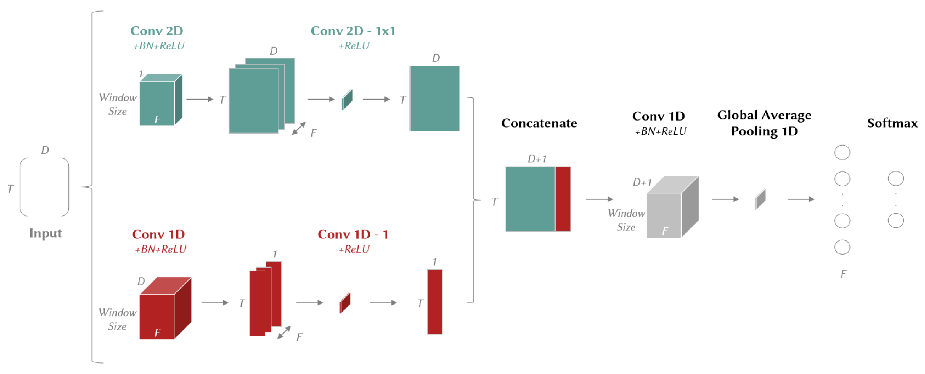
• XCM: we implemented the algorithm with Keras in Python 3.6. 2D convolution layers with: 128 feature maps, kernel size: $WindowSize\times 1$, strides $1\times 1$, padding same and ReLU activation. In addition, 1D convolution layers with: 128 feature maps, kernel size: $WindowSize$, strides 1, padding same and ReLU activation. The hyperparameters are: batch size $\{1,8,32\}$ and $WindowSize$ (the time window size—kernel size), expressed as a percentage of the total size of the MTS $[20\%,40\%,60\%,80\%,100\%]$;
• XCM-Seq: XCM variant with 2D and 1D convolution blocks in sequence (see description in Section 3.1). We used the same setting as XCM.

All the networks that we implemented (XCM, XCM-Seq and MTEX-CNN) were trained with 100 epochs, the categorical crossentropy loss and the Adam optimization (computing infrastructure: Debian 8 operating system, GPU NVIDIA GeForce RTX 2080 Ti with 11Gb GRAM and 96Gb of RAM). Concerning Grad-CAM, we used the implementation available for Keras (https://github.com/jacobgil/keras-grad-cam (accessed on 1 November 2021)).

4.3. Hyperparameters

For each dataset, hyperparameters were set by grid search based on the best average accuracy following a stratified 5-fold cross-validation on the training set.

4.4. Metrics

For each dataset, we computed the classification accuracy—the metric used to benchmark the MTS classifiers on the public UEA datasets [7]. Then, we presented the average rank and the number of wins/ties to compare the different classifiers on the same datasets. Finally, we presented the critical difference diagram [47], the statistical comparison of multiple classifiers on multiple datasets based on the nonparametric Friedman test, to show the overall performance of XCM. We used the implementation available in R package scmamp (https://www.rdocumentation.org/packages/scmamp/versions/0.2.55/topics/plotCD (accessed on 1 November 2021)).

5. Results

In this section, we first present the performance results of XCM on the public UEA datasets. Then, we illustrate how XCM can reconcile performance and explainability on a synthetic dataset. Finally, we end this section by showing that XCM outperforms the current most accurate state-of-the-art algorithm in a real-world application while providing faithful and more informative explanations.

5.1. Performance

The accuracy results on the public UEA test sets of XCM and the other MTS classifiers are presented in

Table 3. Accuracy results on the UEA MTS datasets. Abbreviations: Batch—Batch Size, DW${}_D$—DTW${}_D$, DW${}_I$—DTW${}_I$, MC—MTEX-CNN, MF—MLSTM-FCN, Win %—Time Window Size, WM—WEASEL+MUSE and XC—XCM.

Datasets	XC	XC Seq	MC	MF	WM	ED	DW${}_{\mathit{I}}$	DW${}_{\mathit{D}}$	ED (n)	DW${}_{\mathit{I}}$ (n)	DW${}_{\mathit{D}}$ (n)	XC Parameters
												Batch	Win %
Articulary Word Recognition	98.3	92.7	92.3	98.6	99.3	97.0	98.0	98.7	97.0	98.0	98.7	32	80
Atrial Fibrilation	46.7	33.3	33.3	20.0	26.7	26.7	26.7	20.0	26.7	26.7	22.0	1	60
Basic Motions	100.0	100.0	100.0	100.0	100.0	67.5	100.0	97.5	67.6	100.0	97.5	32	20
Character Trajectories	99.5	98.8	97.4	99.3	99.0	96.4	96.9	99.0	96.4	96.9	98.9	32	80
Cricket	100.0	93.1	90.3	98.6	98.6	94.4	98.6	100.0	94.4	98.6	100.0	32	20
Duck Duck Geese	70.0	52.5	65.0	67.5	57.5	27.5	55.0	60.0	27.5	55.0	60.0	8	80
Eigen Worms	43.5	45.0	41.9	80.9	89.0	55.0	60.3	61.8	54.9		61.8	32	40
Epilepsy	99.3	93.5	94.9	96.4	99.3	66.7	97.8	96.4	66.6	97.8	96.4	32	20
Ering	13.3	13.3	13.3	13.3	13.3	13.3	13.3	13.3	13.3	13.3	13.3	32	20
Ethanol Concentration	34.6	31.6	30.8	29.4	31.6	29.3	30.4	32.3	29.3	30.4	32.3	32	80
Face Detection	63.9	63.8	50.0	57.4	54.5	51.9	51.3	52.9	51.9		52.9	32	60
Finger Movements	60.0	60.0	49.0	61.0	54.0	55.0	52.0	53.0	55.0	52.0	53.0	32	40
Hand Movement Direction	44.6	40.1	18.9	37.8	37.8	27.9	30.6	23.1	27.8	30.6	23.1	32	80
Handwriting	41.2	38.6	24.6	54.9	53.1	37.1	50.9	60.7	20.0	31.6	28.6	32	60
Heartbeat	77.6	74.1	72.2	71.4	72.7	62.0	65.9	71.7	61.9	65.8	71.7	32	80
Insect Wingbeat	10.5	10.5	10.5	10.5		12.8		11.5	12.8			32	20
Japanese Vowels	98.6	94.6	95.1	99.2	97.8	92.4	95.9	94.9	92.4	95.9	94.9	32	80
Libras	84.4	79.4	81.1	92.2	89.4	83.3	89.4	87.2	83.3	89.4	87.0	32	80
LSST	61.2	54.2	31.5	64.6	62.8	45.6	57.5	55.1	45.6	57.5	55.1	32	100
Motor Imagery	54.0	53.0	50.0	53.0	50.0	51.0	39.0	50.0	51.0		50.0	8	40
NATOPS	97.8	93.9	88.3	96.7	88.3	85.0	85.0	88.3	85.0	85.0	88.3	32	40
PenDigits	99.1	96.7	87.8	99.0	96.9	97.3	93.9	97.7	97.3	93.9	97.7	8	60
PEMS-SF	75.7	80.9	11.6	69.9		70.5	73.4	71.1	70.5	73.4	71.1	32	80
Phoneme	22.5	11.9	2.6	27.5	19.0	10.4	15.1	15.1	10.4	15.1	15.1	32	40
Racket Sports	89.5	86.8	82.9	89.4	91.4	86.4	84.2	80.3	86.8	84.2	80.3	32	80
Self Regulation SCP1	87.8	81.6	78.5	86.7	74.4	77.1	76.5	77.5	77.1	76.5	77.5	32	80
Self Regulation SCP2	54.4	55.0	50.0	52.2	52.2	48.3	53.3	53.9	48.3	53.3	53.9	32	80
Spoken Arabic Digits	99.5	99.4	98.6	99.4	98.2	96.7	96.0	96.3	96.7	95.9	96.3	32	80
Stand Walk Jump	40.0	46.7	53.3	46.7	33.3	20.0	33.3	20.0	20.0	33.3	20.0	32	60
U Wave Gesture Library	89.4	81.9	81.2	86.3	90.3	88.1	86.9	90.3	88.1	86.8	90.3	32	100
Average Rank	2.3	5.0	7.2	3.5	4.0	7.1	5.9	4.8	7.4	6.4	5.3
Wins/Ties	16	4	3	7	7	2	2	4	2	2	3

. A blank in the table indicates that the approach ran out of memory. The best accuracy for each dataset is denoted in boldface.

Firstly, we observe that XCM obtains the best average rank and the lowest rank variability across the datasets (rank: 2.3, standard error: 0.4), followed by MLSTM-FCN in second position (rank: 3.5, standard error: 0.5) and WEASEL+MUSE in third position (rank: 4.0, standard error: 0.5). Using the categorization of the datasets published in the archive website (http://www.timeseriesclassification.com/dataset.php (accessed on 1 November 2021)), we do not see any influence from the different train set sizes, MTS lengths, number of dimensions, number of classes and dataset types on XCM performance relative to the other classifiers on the UEA datasets.

More specifically, XCM exhibits better performance than MLSTM-FCN and WEASEL +MUSE on both the large (rank: 1.9, MLSTM-FCN rank: 2.1, WEASEL+MUSE rank: 4.6-train size ≥ 500, 23% of the datasets) and small datasets (rank: 2.4, MLSTM-FCN rank: 4.0, WEASEL+MUSE rank: 3.9-train size < 500, 77% of the datasets). We can assume that the more compact architecture of XCM compared to the other deep learning classifiers provides a better generalization ability on the UEA datasets (average rank on the number of trainable parameters: XCM 1.7, MLSTM-FCN: 1.9, MTEX-CNN: 2.0). Furthermore, the results confirm the superiority of the XCM approach based on the extraction in parallel and directly from the input data of features relative to the observed variables and time compared to the sequential approaches. XCM outperforms both XCM-Seq and MTEX-CNN on average on the UEA datasets (rank: 2.3, XCM-Seq: 5.0, MTEX-CNN: 7.2).

With regard to the hyperparameter $WindowSize$ of XCM, Figure 3 shows the average relative drop in performance across the datasets when using the other time window sizes than the one used in the best configuration given in Table 3. In order to evaluate the relative impact with respect to the range of performance, we defined four categories of datasets: datasets with XCM original accuracy < 50%, datasets with 50% ≤ accuracy < 75%, datasets with 75% ≤ accuracy < 90% and datasets with accuracy ≥ 90%. First, as expected, we observe that the average relative impact of using suboptimal time window sizes is higher when XCM level of performance is low (average relative drop in accuracy: 13.1% when XCM accuracy < 50% versus 3.0% when XCM accuracy ≥ 90%). Then, the average relative drop in accuracy when using suboptimal time window sizes is not negligible but remains limited in all the cases. This drop is below 15% on average on the category where XCM has the lowest level of accuracy (13.1% ± 3.2%) and below 10% on average across all the datasets (7.0% ± 1.3%).

Finally, we performed a statistical test to evaluate the performance of XCM compared to the other MTS classifiers. We present in Figure 4 the critical difference plot with alpha equals to 0.05 from results shown in Table 3. The values correspond to the average rank, and the classifiers linked by a bar do not have a statistically significant difference. The plot confirms the top three ranking as presented before (XCM: 1, MLSTM-FCN: 2, and WEASEL+MUSE: 3), without showing a statistically significant difference between each other. We notice that XCM is the only classifier with a significant performance difference compared to DTW${}_D$.

5.2. Explainability

In this section, we illustrate how our approach XCM reconciles performance and explainability and show that XCM enables a more precise identification of the regions of the input data that are important for predictions compared to the current deep learning MTS classifier also providing faithful explainability—MTEX-CNN. We perform the comparison on a synthetic dataset as the construction of such a dataset allows us to know the expected explanations, with such information not being available in the public UEA datasets. Concerning the evaluation of the results, we adopt the intersection-over-union as a metric, i.e., the extent of overlap between the predicted and expected explanations.

The synthetic dataset is composed of 20 MTS (50%/50% train/test split) with a length of 100, two dimensions, and two balanced classes. The difference between the 10 MTS belonging to the negative class and the one belonging to the positive class stems from a 20% time window of the MTS. Negative class MTS are sine waves, and as illustrated in the plot on the top part of Figure 5, positive class MTS are sine waves with a square signal on 20% of the dimension 1 (see timestamps between 60 and 80).

First, MTEX-CNN and XCM ($BatchSize$: 1, $WindowSize$: 20%) correctly predict the 10 MTS of the test set (accuracy 100%). We observe that XCM and MTEX-CNN obtain the same performance whereas XCM has around 10 times fewer parameters than MTEX-CNN (trainable parameters: XCM 17k, MTEX-CNN 232k).

Moreover, MTEX-CNN and XCM with Grad-CAM all correctly identify the discriminative time window. However, as shown in Figure 5, the attribution maps of MTEX-CNN and XCM with the same explainability method (Grad-CAM) are different. Figure 5 shows one MTS sample belonging to the positive class, and the time and observed variables attribution maps supporting MTEX-CNN and XCM predictions. Attribution maps are heatmaps of the same size as the input data. The more intense the red, the stronger the features (observed variables, time) positively contribute to the prediction. We observe that the attribution maps drawn from XCM are more precise than the ones from MTEX-CNN, i.e., the intersection-over-union of the explanations is higher for XCM than for MTEX-CNN (intersection-over-union: XCM 0.65 versus MTEX-CNN 0.4). On the time attribution map, high attribution values (above 0.6) for XCM begin on timestamp 63 and end on timestamp 76 (expected: $[60,80]$, intersection-over-union: 0.65), whereas for MTEX-CNN they begin later (timestamp 68, intersection-over-union: 0.4). Concerning the attribution map of the observed variables, as expected, we see that high attributions values on the discriminative dimension (dimension 1) appear at the same timestamps as high attribution values on the time attribution map for XCM (timestamps 63 and 76, intersection-over-union: 0.65). Nonetheless, the observed variables attribution map of MTEX-CNN shows high attribution values on a window larger than the discriminative one (timestamps range $[34,83]$, intersection-over-union: 0.41). As MTEX-CNN attribution maps exhibit a red color gradient, the precision of identification of the regions of the input data on MTEX-CNN attribution maps could be enhanced by setting a higher threshold than 0.6 for the attribution values. However, the red color gradient is due to the upsampling processes needed to match the 2D/1D output features maps of MTEX-CNN to the size of the input data when applying Grad-CAM. Grad-CAM is applied at a local level, which means that we would need to potentially set a different threshold for each instance and that would render MTEX-CNN explainability method impractical. Thus, based on the same attribution threshold (0.6), XCM allows a more precise identification of the regions of the input data that are important for predictions than MTEX-CNN. Both MTEX-CNN and XCM have periodically high attribution values on dimension 2 of the observed variables attribution maps. It could be surprising as the sinusoidal signal on this dimension is the same across all MTS; however, the fact that this information is uniformly high or low renders it irrelevant for explanations. Therefore, considering that XCM-Seq attributions maps are the same as XCM ones, we can assume that the use of half padding on the different convolution layers to reduce the number of parameters in MTEX-CNN, i.e., the use of upsampling to retrieve the input data dimensions on the attribution maps, can lead to a less precise identification of the regions of the input data that are important for predictions.

5.3. Real-World Application

Machine learning methods have great potential to improve the detection of determining events for milk production in dairy farms, which is one of the most important steps toward meeting both food production and environmental goals [48]. A key factor for dairy farms performance is reproduction. Reproduction directly impacts milk production as cows start to produce milk after giving birth to a calf; and milk productivity declines after the first 3 months. Furthermore, the most prevalent reason for cow culling, the act of slaughtering a cow, is a reproduction issue (e.g., long interval between two calves) [49]. Thus, it is crucial to detect estrus, the only period when the cow is susceptible to pregnancy, to timely inseminate cows and therefore optimize resource use in dairy farms.

The ground truth is estrus estimation using automated progesterone analysis in milk [50,51]. However, the cost of this solution prohibits its extensive implementation. Thus, the machine learning challenge lies in developing a binary MTS classifier to detect estrus (class estrus/non-estrus) based on affordable sensor data (activity and body temperature). Commercial solutions based on these affordable sensor data have been developed. Nonetheless, their adoption rate remains moderate [52]. These commercial detection solutions suffer from insufficient performance (false alerts and incomplete estrus coverage) and from a lack of justifications supporting alerts. Therefore, aside from an enhanced performance, decision support solutions need to provide to the farmers some explanations supporting the alerts.

The offline dataset consists of 15.5k MTS samples of length 4 with seven variables: the body temperature variable and six activity variables (rumination, ingestion, rest, standing up, over activity and other activity). A time series corresponds to a 4 day period (MTS length 4): the day of estrus (Day 0) and the previous 3 days. The labels are set with the ground truth in estrus detection—progesterone dosage in whole milk. We compare XCM with Grad-CAM to a reference commercial solution (HeatPhone [53]) and the most accurate state-of-the-art MTS classifier of our benchmark (see Section 4.2) on this real-world application—MLSTM-FCN—with SHAP [32]. As far as we have seen, an architecture concatenating a LSTM network with a CNN such as MLSTM-FCN can only rely on post hoc model-agnostic explainability methods to support its predictions. We chose the state-of-the-art explainability method SHAP as its granularity of explanation is comparable to Grad-CAM (both global and local). Indeed, Grad-CAM can also offer global explainability by averaging the attribution maps values per class. SHAP provides the relative importance of the observed variables and timestamps on predictions. Performance is calculated following a five-fold cross-validation and an arithmetic mean of the F1-scores on test sets. The choice of this metric is driven by two reasons. First, no assumption is made about the dairy management style; farmers can favor a higher estrus detection rate (higher recall) or fewer false alerts (higher precision) according to their needs. Second, there is a class imbalance (33% of estrus days) which renders irrelevant the accuracy metric.

As presented in

Table 4. Estrus detection F1-score on test sets with 95% confidence interval.

	XCM	MLSTM-FCN	Commercial Solution
F1-Score	69.7 ± 1.5	63.1 ± 1.5	55.3 ± 5.1

, we observe that XCM outperforms the current state-of-the-art deep learning approach (MLSTM-FCN) and the reference commercial solution by increasing the average F1-score (69.7% versus 63.1 % and 55.3%) and obtaining the lowest variability across folds (1.5% versus 1.5% and 5.1%). In addition, concerning XCM explainability, Figure 6 shows an example of the observed variables and time attribution maps supporting the correct prediction of an MTS sample belonging to the class Estrus. We plot the MTS sample with a heatmap to ease the readability. The intersection of attribution maps and sample values inform us that the prediction was made mainly based on the presence of a high overactivity (or low rest) of the animal on the day of estrus (attribution values above 0.6 on Day 0 and on the variable over activity, which has a high value). This behavior is aligned with the literature on estrus detection [54], as it is the behavior associated with most of the estrus.

The current state-of-the-art MTS classifiers MLSTM-FCN and XCM have different explainability methods (SHAP—post hoc model-agnostic, Grad-CAM—post hoc model-specific) which come with their own form of explanations. In order to assess and benchmark these two MTS classifiers also with respect to their explainability, we use a framework that we have proposed in [55]. The framework details a set of characteristics (performance, model comprehensibility, granularity of the explanations, information type, faithfulness and user category) that systematize the performance-explainability assessment of machine learning methods. The results of the framework are represented in a parallel coordinates plot in Figure 7. Both deep learning approaches are hard-to-understand models (Comprehensibility: Black-Box) which provide explanations at both global and local levels (Granularity: Global and Local) that can be analyzed by a domain expert (User: Domain Expert). However, in addition to giving the relative importance of observed variables and time as MLSTM-FCN with SHAP, XCM with Grad-CAM provides more informative explanations by supplying the corresponding sample values (Information: MLSTM-FCN with SHAP—Features+Time and XCM with Grad-CAM—Features+Time+Values). Furthermore, unlike MLSTM-FCN with SHAP and as discussed in Section 2.3, XCM with Grad-CAM approach provides faithful explanations, which is a prerequisite to reduce solution mistrust from the farmers (Faithfulness: MLSTM-FCN with SHAP—Imperfect and XCM with Grad-CAM—Perfect). Therefore, XCM outperforms the current state-of-the-art algorithm on the real-world application (Performance: Best), while enhancing explainability by providing faithful and more informative explanations.

Finally, the performance-explainability framework introduced in the previous paragraph can also be used to identify the limitations of XCM, which point to the directions to improve our approach. We see in Figure 7 that the level of information of the explanation provided by XCM with Grad-CAM (Features+Time+Values) could be enhanced. Therefore, aside from automating the hyperparameter setting of XCM ($WindowSize$), it would be interesting to work on synthesizing the attribution maps to improve the level of information.

6. Conclusions

We have presented XCM, a new compact and explainable convolutional neural network for MTS classification, which extracts information relative to the observed variables and time directly from the input data. XCM exhibits a better average rank than the state-of-the-art classifiers on both the large and small public UEA datasets. Moreover, it was designed to enable faithful explainability based on Grad-CAM method and the precise identification of the regions of the input data that are important for predictions. Following the illustration of the performance and explainability of XCM on a synthetic dataset, we showed how XCM can outperform the current most accurate state-of-the-art algorithm MLSTM-FCN on a real-world application while enhancing explainability by providing faithful and more informative explanations.

In our future work, we would like to automate XCM hyperparameter setting ($WindowSize$) and evaluate the impact of different fusion methods of the 2D and 1D feature maps (e.g., weighting scheme) on XCM performance. With regard to explainability, it would be interesting to further enhance the explanations of XCM with Grad-CAM by synthesizing the attribution maps with multidimensional sequential patterns to improve the level of information.

References

1. Chen, C.; Bian, J.; Xing, C.; Liu, T. Investment Behaviors Can Tell What Inside: Exploring Stock Intrinsic Properties for Stock Trend Prediction. In Proceedings of the 25th ACM SIGKDD International Conference on Knowledge Discovery and Data Mining, Anchorage, AK, USA, 4–8 August 2019. [Google Scholar]
2. Li, J.; Rong, Y.; Meng, H.; Lu, Z.; Kwok, T.; Cheng, H. TATC: Predicting Alzheimer’s Disease with Actigraphy Data. In Proceedings of the 24th ACM SIGKDD International Conference on Knowledge Discovery and Data Mining, London, UK, 19–23 August 2018. [Google Scholar]
3. Jiang, R.; Song, X.; Huang, D.; Song, X.; Xia, T.; Cai, Z.; Wang, Z.; Kim, K.; Shibasaki, R. DeepUrbanEvent: A System for Predicting Citywide Crowd Dynamics at Big Events. In Proceedings of the 25th ACM SIGKDD International Conference on Knowledge Discovery and Data Mining, Anchorage, AK, USA, 4–8 August 2019. [Google Scholar]
4. Fauvel, K.; Balouek-Thomert, D.; Melgar, D.; Silva, P.; Simonet, A.; Antoniu, G.; Costan, A.; Masson, V.; Parashar, M.; Rodero, I.; et al. A Distributed Multi-Sensor Machine Learning Approach to Earthquake Early Warning. In Proceedings of the 34th AAAI Conference on Artificial Intelligence, New York, NY, USA, 7–12 February 2020. [Google Scholar]
5. Karim, F.; Majumdar, S.; Darabi, H.; Harford, S. Multivariate LSTM-FCNs for Time Series Classification. Neural Netw. 2019, 116, 237–245. [Google Scholar] [CrossRef] [PubMed] [Green Version]
6. Schäfer, P.; Leser, U. Multivariate Time Series Classification with WEASEL+MUSE. arXiv 2017, arXiv:1711.11343. [Google Scholar]
7. Bagnall, A.; Lines, J.; Keogh, E. The UEA Multivariate Time Series Classification Archive, 2018. arXiv 2018, arXiv:1811.00075. [Google Scholar]
8. Schäfer, P.; Högqvist, M. SFA: A Symbolic Fourier Approximation and Index for Similarity Search in High Dimensional Datasets. In Proceedings of the 15th International Conference on Extending Database Technology, Berlin, Germany, 27–30 March 2012; pp. 516–527. [Google Scholar]
9. Rudin, C. Stop Explaining Black Box Machine Learning Models for High Stakes Decisions and Use Interpretable Models Instead. Nat. Mach. Intell. 2019, 1, 206–215. [Google Scholar] [CrossRef] [Green Version]
10. Selvaraju, R.; Das, A.; Vedantam, R.; Cogswell, M.; Parikh, D.; Batra, D. Grad-CAM: Visual Explanations from Deep Networks via Gradient-Based Localization. Int. J. Comput. Vis. 2019, 128, 336–359. [Google Scholar] [CrossRef] [Green Version]
11. Adebayo, J.; Gilmer, J.; Muelly, M.; Goodfellow, I.; Hardt, M.; Kim, B. Sanity Checks for Saliency Maps. In Proceedings of the 32nd International Conference on Neural Information Processing Systems, Montreal, QC, Canada, 3–8 December 2018. [Google Scholar]
12. Assaf, R.; Giurgiu, I.; Bagehorn, F.; Schumann, A. MTEX-CNN: Multivariate Time Series EXplanations for Predictions with Convolutional Neural Networks. In Proceedings of the IEEE International Conference on Data Mining, Beijing, China, 8–11 November 2019. [Google Scholar]
13. Goodfellow, I.; Bengio, Y.; Courville, A. Deep Learning; MIT Press: Cambridge, MA, USA, 2016. [Google Scholar]
14. Huang, G.; Liu, Z.; Van Der Maaten, L.; Weinberger, K. Densely Connected Convolutional Networks. In Proceedings of the 2017 IEEE Conference on Computer Vision and Pattern Recognition, Honolulu, HI, USA, 21–26 July 2017. [Google Scholar]
15. Sutskever, I.; Vinyals, O.; Le, Q. Sequence to Sequence Learning with Neural Networks. In Proceedings of the 27th International Conference on Neural Information Processing Systems, Montreal, QC, Canada, 8–13 December 2014. [Google Scholar]
16. Devlin, J.; Chang, M.; Lee, K.; Toutanova, K. BERT: Pre-Training of Deep Bidirectional Transformers for Language Understanding. In Proceedings of the 2019 Conference of the North American Chapter of the Association for Computational Linguistics, Minneapolis, MN, USA, 2–7 June 2019. [Google Scholar]
17. Cristian Borges Gamboa, J. Deep Learning for Time-Series Analysis. arXiv 2017, arXiv:1701.01887. [Google Scholar]
18. Seto, S.; Zhang, W.; Zhou, Y. Multivariate Time Series Classification Using Dynamic Time Warping Template Selection for Human Activity Recognition. In Proceedings of the IEEE Symposium Series on Computational Intelligence, Cape Town, South Africa, 7–10 December 2015. [Google Scholar]
19. Vidal, E.; Casacuberta, F.; Segovia, H. Is the DTW “Distance” Really a Metric? An Algorithm Reducing the Number of DTW Comparisons in Isolated Word Recognition. Speech Commun. 1985, 4, 333–344. [Google Scholar] [CrossRef]
20. Shokoohi-Yekta, M.; Hu, B.; Jin, H.; Wang, J.; Keogh, E. Generalizing DTW to the Multi-Dimensional Case Requires an Adaptive Approach. Data Min. Knowl. Discov. 2017, 31, 1–31. [Google Scholar] [CrossRef] [PubMed] [Green Version]
21. Karlsson, I.; Papapetrou, P.; Boström, H. Generalized Random Shapelet Forests. Data Min. Knowl. Discov. 2016, 30, 1053–1085. [Google Scholar] [CrossRef]
22. Wistuba, M.; Grabocka, J.; Schmidt-Thieme, L. Ultra-Fast Shapelets for Time Series Classification. arXiv 2015, arXiv:1503.05018. [Google Scholar]
23. Baydogan, M.; Runger, G. Time Series Representation and Similarity Based on Local Autopatterns. Data Min. Knowl. Discov. 2016, 30, 476–509. [Google Scholar] [CrossRef]
24. Tuncel, K.; Baydogan, M. Autoregressive Forests for Multivariate Time Series Modeling. Pattern Recognit. 2018, 73, 202–215. [Google Scholar] [CrossRef]
25. Baydogan, M.; Runger, G. Learning a Symbolic Representation for Multivariate Time Series Classification. Data Min. Knowl. Discov. 2014, 29, 400–422. [Google Scholar] [CrossRef]
26. Wang, Z.; Yan, W.; Oates, T. Time Series Classification from Scratch with Deep Neural Networks: A Strong Baseline. In Proceedings of the 2017 International Joint Conference on Neural Networks, Anchorage, AK, USA, 14–19 May 2017. [Google Scholar]
27. He, K.; Zhang, X.; Ren, S.; Sun, J. Deep Residual Learning for Image Recognition. In Proceedings of the 2016 IEEE Conference on Computer Vision and Pattern Recognition, Las Vegas, NV, USA, 27–30 June 2016. [Google Scholar]
28. Zhang, X.; Gao, Y.; Lin, J.; Lu, C. TapNet: Multivariate Time Series Classification with Attentional Prototypical Network. In Proceedings of the 34th AAAI Conference on Artificial Intelligence, New York, NY, USA, 7–12 February 2020. [Google Scholar]
29. Zerveas, G.; Jayaraman, S.; Patel, D.; Bhamidipaty, A.; Eickhoff, C. A Transformer-Based Framework for Multivariate Time Series Representation Learning. In Proceedings of the 27th ACM SIGKDD Conference on Knowledge Discovery and Data Mining, Virtual Event, 14–18 August 2021. [Google Scholar]
30. Du, M.; Liu, N.; Hu, X. Techniques for Interpretable Machine Learning. Commun. ACM 2020, 63, 68–77. [Google Scholar] [CrossRef] [Green Version]
31. Ribeiro, M.; Singh, S.; Guestrin, C. “Why Should I Trust You?”: Explaining the Predictions of Any Classifier. In Proceedings of the 22nd ACM SIGKDD International Conference on Knowledge Discovery and Data Mining, San Francisco, CA, USA, 13–17 August 2016. [Google Scholar]
32. Lundberg, S.; Lee, S. A Unified Approach to Interpreting Model Predictions. In Proceedings of the 31st International Conference on Neural Information Processing Systems, Long Beach, CA, USA, 4–9 December 2017. [Google Scholar]
33. Ribeiro, M.; Singh, S.; Guestrin, C. Anchors: High-Precision Model-Agnostic Explanations. In Proceedings of the 32nd AAAI Conference on Artificial Intelligence, New Orleans, LA, USA, 2–7 February 2018. [Google Scholar]
34. Guidotti, R.; Monreale, A.; Giannotti, F.; Pedreschi, D.; Ruggieri, S.; Turini, F. Factual and Counterfactual Explanations for Black Box Decision Making. IEEE Intell. Syst. 2019, 34, 14–23. [Google Scholar] [CrossRef]
35. Ancona, M.; Ceolini, E.; Öztireli, C.; Gross, M. Towards Better Understanding of Gradient-Based Attribution Methods for Deep Neural Networks. In Proceedings of the International Conference on Learning Representations, Vancouver, BC, Canada, 1–3 May 2018. [Google Scholar]
36. Erhan, D.; Bengio, Y.; Courville, A.; Vincent, P. Visualizing Higher-Layer Features of a Deep Network. In Proceedings of the ICML Workshop on Learning Feature Hierarchies, Montreal, QC, Canada, 9 June 2009. [Google Scholar]
37. Springenberg, J.; Dosovitskiy, A.; Brox, T.; Riedmiller, M. Striving for Simplicity: The All Convolutional Net. In Proceedings of the International Conference on Learning Representations (Workshop Track), San Diego, CA, USA, 7–9 May 2015. [Google Scholar]
38. Bach, S.; Binder, A.; Montavon, G.; Klauschen, F.; Müller, K.; Samek, W. On Pixel-Wise Explanations for Non-Linear Classifier Decisions by Layer-Wise Relevance Propagation. PLoS ONE 2015, 10, e0130140. [Google Scholar] [CrossRef] [PubMed] [Green Version]
39. Shrikumar, A.; Greenside, P.; Shcherbina, A.; Kundaje, A. Not Just a Black Box: Learning Important Features Through Propagating Activation Differences. arXiv 2016, arXiv:1605.01713. [Google Scholar]
40. Sundararajan, M.; Taly, A.; Yan, Q. Axiomatic Attribution for Deep Networks. In Proceedings of the 34th International Conference on Machine Learning, Sydney, Australia, 6–11 August 2017. [Google Scholar]
41. Shrikumar, A.; Greenside, P.; Kundaje, A. Learning Important Features through Propagating Activation Differences. In Proceedings of the 34th International Conference on Machine Learning, Sydney, Australia, 6–11 August 2017. [Google Scholar]
42. Lin, M.; Chen, Q.; Yan, S. Network in Network. arXiv 2014, arXiv:1312.4400. [Google Scholar]
43. Ioffe, S.; Szegedy, C. Batch Normalization: Accelerating Deep Network Training by Reducing Internal Covariate Shift. In Proceedings of the 32nd International Conference on Machine Learning, Lille, France, 6–11 July 2015. [Google Scholar]
44. Nair, V.; Hinton, G. Rectified Linear Units Improve Restricted Boltzmann Machines. In Proceedings of the 27th International Conference on Machine Learning, Haifa, Israel, 21–24 June 2010. [Google Scholar]
45. Bjorck, N.; Gomes, C.; Selman, B.; Weinberger, K. Understanding Batch Normalization. In Proceedings of the 32nd International Conference on Neural Information Processing Systems, Montreal, QC, Canada, 3–8 December 2018. [Google Scholar]
46. Szegedy, C.; Liu, W.; Jia, Y.; Sermanet, P.; Reed, S.; Anguelov, D.; Erhan, D.; Vanhoucke, V.; Rabinovich, A. Going Deeper with Convolutions. In Proceedings of the IEEE Conference on Computer Vision and Pattern Recognition, Boston, MA, USA, 7–12 June 2015. [Google Scholar]
47. Demšar, J. Statistical Comparisons of Classifiers over Multiple Data Sets. J. Mach. Learn. Res. 2006, 7, 1–30. [Google Scholar]
48. Searchinger, T.; Waite, R.; Hanson, C.; Ranganathan, J.; Dumas, P.; Matthews, E. Creating a Sustainable Food Future; World Resources Institute: Washington, DC, USA, 2018. [Google Scholar]
49. Bascom, S.; Young, A. A Summary of the Reasons Why Farmers Cull Cows. J. Dairy Sci. 1998, 81, 2299–2305. [Google Scholar] [CrossRef]
50. Cutullic, E.; Delaby, L.; Gallard, Y.; Disenhaus, C. Dairy Cows’ Reproductive Response to Feeding Level Differs According to the Reproductive Stage and the Breed. Animal 2011, 5, 731–740. [Google Scholar] [CrossRef] [PubMed]
51. Tenghe, A.; Bouwman, A.; Berglund, B.; Strandberg, E.; Blom, J.; Veerkamp, R. Estimating genetic parameters for fertility in dairy cows from in-line milk progesterone profiles. J. Dairy Sci. 2015, 98, 5763–5773. [Google Scholar] [CrossRef] [Green Version]
52. Steeneveld, W.; Hogeveen, H. Characterization of Dutch Dairy Farms Using Sensor Systems for Cow Management. J. Dairy Sci. 2015, 98, 709–717. [Google Scholar] [CrossRef] [PubMed]
53. Chanvallon, A.; Coyral-Castel, S.; Gatien, J.; Lamy, J.; Ribaud, D.; Allain, C.; Clément, P.; Salvetti, P. Comparison of Three Devices for the Automated Detection of Estrus in Dairy Cows. Theriogenology 2014, 82, 734–741. [Google Scholar] [CrossRef] [PubMed]
54. Gaillard, C.; Barbu, H.; Sørensen, M.; Sehested, J.; Callesen, H.; Vestergaard, M. Milk Yield and Estrous Behavior During Eight Consecutive Estruses in Holstein Cows Fed Standardized or High Energy Diets and Grouped According to Live Weight Changes in Early Lactation. J. Dairy Sci. 2016, 99, 3134–3143. [Google Scholar] [CrossRef] [PubMed] [Green Version]
55. Fauvel, K.; Masson, V.; Fromont, É. A Performance-Explainability Framework to Benchmark Machine Learning Methods: Application to Multivariate Time Series Classifiers. In Proceedings of the IJCAI-PRICAI 2020 Workshop on Explainable AI, Virtual Event, 8 January 2021. [Google Scholar]
Figure 1. MTEX-CNN architecture. Abbreviations: D—number of observed variables, de—dense layer size, F—number of filters, k—kernel size and T—time series length.
Mathematics 09 03137 g001
Figure 2. XCM architecture. Abbreviations: BN—Batch Normalization, D—number of observed variables, F—number of filters, T—time series length and Window Size—kernel size, which corresponds to the time window size.
Mathematics 09 03137 g002
Figure 3. XCM average relative accuracy drop across the UEA datasets when using other time window sizes than the one used in the best configuration given in Table 3. The performance drop is presented across four categories of datasets, defined according to XCM levels of accuracy shown in Table 3. Abbreviation: Acc—Accuracy.
Mathematics 09 03137 g003
Figure 4. Critical difference plot of the MTS classifiers on the UEA datasets with alpha equal to 0.05.
Mathematics 09 03137 g004
Figure 5. Observed variables and time attribution maps supporting the correct MTEX-CNN and XCM predictions of an MTS from the synthetic dataset belonging to the class Positive. Abbreviation: Dim—Dimension.
Mathematics 09 03137 g005
Figure 6. Observed variables and time attribution maps supporting the correct XCM prediction of an MTS from the real-world test set, which belongs to the class Estrus. The MTS sample is represented under the form of a heatmap with the regions important for the prediction highlighted with a red square.
Mathematics 09 03137 g006
Figure 7. Parallel coordinates plot of XCM and the state-of-the-art MTS classifiers on the real-world application. Performance evaluation method: 5-fold cross-validation and an arithmetic mean of the F1-scores. As presented in Section 2.2, the models evaluated in the benchmark are: DTW D , DTW I , FCN, gRSF, LPS, MLSTM-FCN, MTEX-CNN, mv-ARF, ResNet, SMTS, UFS, WEASEL+MUSE and XCM.
Mathematics 09 03137 g007