1. Introduction
The term
rectifying curve was introduced by Chen in [
1] to designate a curve whose position vector always lies in its rectifying plane. Kim et al. [
2] also studied the properties of the “space curves satisfying
”. They proved that a curve has this property if and only if there exists a point such that all of the rectifying planes to the curve pass through this point. By a translation, any curve of this type turns out to be a
rectifying curve in the restricted sense of [
1]. In this paper, we consider, for a rectifying curve, the definition from [
2] because it employs only the intrinsic properties of the curve.
The geometric properties of rectifying curves are presented in detail in [
1,
3]. It is shown that any rectifying curve has a parametrization of the form
where
is a unit speed curve on the unit sphere
,
and
are some constants. Chen [
4] proved that a geodesic on a conical surface is either a rectifying curve or an open portion of a ruling.
The relationship between rectifying curves and the notion of centrodes in mechanics is pointed out in [
3] and developed in [
5]. The
centrode of a curve is the curve defined by the Darboux vector
. Chen and Dillen showed in [
3] that the centrode of a unit speed curve with constant (nonzero) curvature and nonconstant torsion is a rectifying curve (and the same result holds for a curve with constant (nonzero) torsion and nonconstant curvature). A generalization of these results is given in [
5], where it is proven that the centrode of a twisted nonhelical curve is a rectifying curve if and only if the curvature
and torsion
are not both constants and if they satisfy a nonhomogeneous linear equation of the form
, where
and
. In the same paper, Deshmukh et al. show that, for any twisted nonhelical curve, the dilated centrode
is a rectifying curve.
In this paper, we give a new characterization of rectifying curves based on the relationship with their evolutes/involutes. An involute of a curve is a curve that lies on the tangent surface to and intersects the tangent lines orthogonally. If the curve is an involute of , then is said to be an evolute of . We prove that a curve is a rectifying curve if and only if it has a spherical involute (see Corollary 2). We also express the curvature and the torsion of a spherical rectifying curve (in Theorem 3) and give necessary and sufficient conditions for a curve and its involute to be both rectifying curves (in Theorem 5). A direct consequence of Theorem 6 is that rectifying curves can be constructed as evolutes of spherical non-planar curves.
The outline of the paper is as follows.
Section 2 contains some basic notions and formulas needed for our work. In
Section 3, we briefly present the main features of rectifying curves and give (in Theorem 3) necessary and sufficient conditions for a rectifying curve to lie on a sphere.
Section 4 is devoted to the involute of a rectifying curve and establishes in which conditions an involute of a rectifying curve is also a rectifying curve. In
Section 5, we state and prove a new defining feature of rectifying curves: a curve is a rectifying curve if and only if its involutes are spherical curves. This result (Theorem 6) allows us to develop a new method of constructing rectifying curves: as evolutes of spherical twisted curves. The method is applied in
Section 6 to construct rectifying curves as evolutes of a spherical helix.
2. Preliminaries
We denote by the Euclidean 3-space with its inner product .
Let I be a real interval and be a space curve of class , parametrized by the arc-length s (a unit-speed curve). The unit vector field is called the tangent vector field. The curvature of the curve is the positive function . We assume that for any and define the principal normal vector field as . Since for all , it follows that ; hence, is orthogonal to . The binormal vector field is defined by the cross product . It is a unit vector field orthogonal to both and . The torsion of the curve is the function by the equation . The orthogonal unit vectors , and form the well-known Frenet frame or Frenet trihedron.
The vector fields
,
and
satisfy the following
Frenet–Serret formulas (see, for instance, [
6] or [
7]):
At each point of the curve, the planes determined by , and are known as the osculating plane, the rectifying plane and the normal plane, respectively. A curve in is called twisted if it has nonzero curvature and torsion.
3. Rectifying Curves
In the following, we consider to be a unit speed curve of class with for all .
Definition 1. A curve is a rectifying curve if there exists a point that belongs to all of the rectifying planes to the curve. The point (uniquely determined) is said to be the reference point of the rectifying curve (see [4]). By Definition 1, a rectifying curve can be written as:
for any
, where
are functions of class
. These functions cannot be arbitrary; they have a well-defined form established by the following theorem (see [
1,
2]):
Theorem 1. The unit speed curve is a rectifying curve if and only if there exist and the constants , , such that A rectifying curve can also be defined by the ratio
. It is known that a space curve is said to be a a generalized helix if and only if the ratio
is a nonzero constant. For rectifying curves, the ratio
must be a (nonconstant) linear function of the arc-length
s. Thus, by a simple differentiation of (
3) and using Frenet–Serret Formula (
1), we obtain that
so
and the next theorem follows (see also [
1,
2]):
Theorem 2. The unit speed curve is a rectifying curve if and only if there exist the constants , , such that The first main result of the paper is the following theorem, which gives necessary and sufficient conditions for a rectifying curve to lie on a sphere.
Theorem 3. A unit speed rectifying curve lying on a sphere of radius r has the curvature and torsion expressed by the following equations:where and . Conversely, if the curvature and the torsion of a curve are given by (7) and (8), then it is a spherical rectifying curve. Proof. Let
be a unit speed rectifying curve that lies on a sphere of radius
r, centered at
. Thus,
By differentiating the relation above, we obtain that
so we can write
where
and
are two functions, such that
We differentiate (
11) and use Frenet–Serret Formula (
1):
so we obtain:
From (
14), we have
and, after replacing in (16), we obtain:
Since
is a rectifying curve, by Theorem 2, there exist
with
, such that the ratio
satisfies Equation (
6). Hence, Equation (
18) is written
and we obtain by integration that
where
is a constant. From Equation (
12), we obtain that
so the Formula (
7) readily follows. For Equation (
8), we simply apply (
6).
Conversely, let
be a curve with the curvature
and the torsion
be given by the Formulas (
7) and (
8). Then
, hence
is a rectifying curve. It can also be proven, by a straightforward calculation, that
and
satisfy the equation
so the curve
lies on a sphere of radius
r ([
7], p. 32). □
4. The Involute of a Rectifying Curve
An involute of a curve
is a curve
lying on the surface generated by the tangent lines to
, and having the property that these tangent lines are orthogonal to the corresponding tangent lines to
(see [
6,
7]). It can be proven that
is of the form:
where
is a constant.
If
is a rectifying curve defined by (
3) and
is one of its involutes, defined by (
22), then
so
and the following theorem is proven:
Theorem 4. Any involute of a rectifying curve lies on a sphere centered at the reference point.
The next theorem establishes in which conditions an involute of a rectifying curve is also a rectifying curve.
Theorem 5. Let be a rectifying curve (satisfying Equation (6)). Letbe an involute of ( is a constant). Then, is also a rectifying curve if and only if the curvature of the curve is expressed by:where δ and γ are real constants, . Proof. Assume that on I.
Let
be the arc-length parameter of
. Then, since
,
hence
We can write the unit vectors of the Frenet trihedron of the curve
as follows. Obviously,
, and we have:
Thus, the relationship between the Frenet frames
and
can be written:
and the curvature
and the torsion
of
are given by the formulas (see also [
8]):
However,
is a rectifying curve, so we can write, by Equation (
6),
The involute
is a rectifying curve if and only if
It follows that the curvature
must satisfy the following (Bernoulli) differential equation:
The general solution of this equation is given by Formula (
26), where
, and so the proof is complete. □
Remark 1. If we look at Formula (33), we can say that (because ), so we conclude that the involute of a rectifying curve is always a non-planar curve. Corollary 1. If a rectifying curve has an involute that is a rectifying curve, then any other involute of is not a rectifying curve.
Proof. Suppose that
and
are two involutes of the rectifying curve
, which are also rectifying curves. Then, the differential Equation (
37) must be satisfied for
,
and for
,
, respectively. It follows that
hence
and
(the two curves coincide). □
Remark 2. If the curve and its involute are both rectifying curves, they cannot have the same reference point.
Indeed, if we suppose that is the reference point of both curves, they could be written:where is the arc-length parameter of the curve , and , are constants. Thus, we could write: However, since , the equation above implies that , which is not possible.
5. The Evolute of a Rectifying Curve
Recall that an evolute of a curve is a curve with the property that is an involute of .
Let
, be a unit speed curve with the Frenet frame
, the curvature
and the torsion
. If
is an evolute of
, then the vector
is orthogonal to
, so
where
and
are two functions such that, for any
, the vector
is collinear to
. We differentiate (
44) with respect to
s, the arc-length parameter of the curve
:
Thus, the vector
has the expression:
Since
and
are collinear vectors, by (
44) and (
46), we obtain:
and
From the last equation we have
so
We integrate this equation and, using (
47), we find:
where
is a primitive of the torsion
. Thus, the expression of
is:
so any evolute of the curve
has the expression:
Remark 3. By Theorem 4 and Remark 1, if the evolute of a curve is a rectifying curve, then must be a non-planar curve that lies on a sphere centered at the reference point of . We prove in the next theorem that any evolute of any spherical non-planar curve is a rectifying curve.
Theorem 6. The evolutes of a spherical non-planar curve are rectifying curves with the reference point at the center of the sphere.
Proof. Suppose that
is a unit speed curve lying on a sphere centered at
. If
is the Frenet frame,
is the curvature and
is the torsion of
, then, by Equations (
11), (
14) and (
15), we can write:
where
and
. Thus, we have:
Let
be an evolute of
. Then, by Equation (
53), one can write:
where
is a primitive of the torsion
.
Let
denote the unit vectors of the Frenet frame and
denote the curvature and the torsion of the curve
. By Formula (
31), since
is an involute of
, we have:
and so Equation (
56) is written:
Hence, is a rectifying curve with the reference point . □
Following on from Theorems 4 and 6, the next corollary establishes a new defining feature of rectifying curves:
Corollary 2. A curve is a rectifying curve if and only if it has a spherical involute. In this case, the reference point of is the center of the sphere and all of the involutes of lie on concentric spheres centered at this point.
6. Construction of Rectifying Curves
To date, there exist two main sources for the construction of rectifying curves: as dilations of unit speed, spherical curves (see Theorem 7), or as (dilated) centrodes of some type of curves (see Theorems 8 and 9).
Theorem 7 ([
3,
5])
. If is a unit speed curve that lies on the unit sphere and is not an arc of a great circle, then the curve is defined bywhere , is a rectifying curve. Theorem 8 ([
5])
. If is a unit speed curve that is neither a planar curve nor a helix, such that the curvature κ and torsion τ are not both constants and satisfy a nonhomogeneous linear equation of the form , where and , then the centrode of ,is a rectifying curve. Theorem 9 ([
5])
. If is a unit speed curve that is neither a planar curve nor a helix, then the dilated centrodeis a rectifying curve. By Theorem 6, we introduce a new method for constructing rectifying curves: as evolutes of spherical twisted curves. We illustrate this method with the following example:
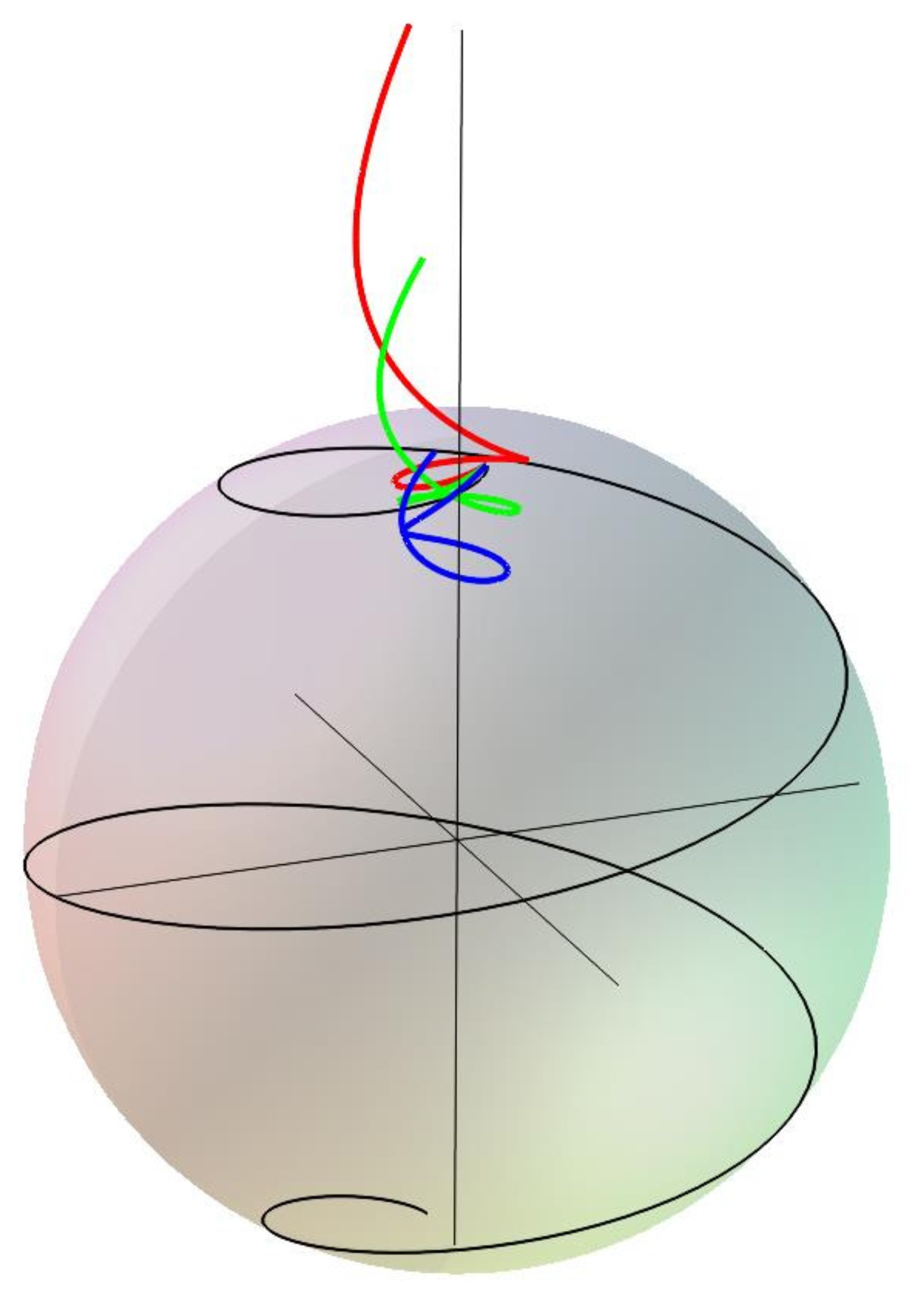
Example 1. Consider the spherical helix that lies on the unit sphere :, . The unit vectors of the Frenet frame of the curve are:and the curvature and the torsion are given by the formulas: Let s denote the arc-length parameter of : We use the Formula (53) to construct an evolute of , which is, by Theorem 6, a rectifying curve. Let be a primitive of the torsion , . We have:where C is a constant. Thus, the following family of rectifying curves is obtained: We remark that any rectifying curve defined by (67) can be written as a dilation of a unit speed circle on the sphere , Thus, if we denote , we can write: We also note that all of the rectifying curves defined by (67) lie on the cone of equation Moreover, as Chen proved in [4], they are geodesics on this cone. In Figure 1, we represented the spherical helix defined by (62) (for ) and three rectifying curves (evolutes of given by the Formula (67), obtained for , and , respectively). 7. Conclusions
In this paper, we state and prove some new properties of rectifying curves based on the relationship with their involutes/evolutes. Thus, we express the curvature and the torsion of a rectifying spherical curve and give necessary and sufficient conditions for a curve and its involute to be both rectifying curves.
We also give a new characterization of rectifying curves: we prove that a necessary and sufficient condition for a curve to be a rectifying curve is for it to posses a spherical involute. Consequently, rectifying curves can be constructed as evolutes of spherical twisted curves. We apply this method to construct the rectifying curves obtained as the evolutes of a spherical helix.
Author Contributions
Conceptualization, M.J., S.A. and A.M.; methodology, M.J., S.A., L.D., A.M. and D.T.; validation, L.D., O.-A.R. and D.T.; writing—original draft preparation, M.J.; writing—review and editing, M.J., S.A., L.D., A.M., O.-A.R. and D.T.; supervision, A.M.; project administration, A.M. All authors have read and agreed to the published version of the manuscript.
Funding
This research was supported by the internal competition in the Technical University of Civil Engineering Bucharest, based on special funding for academic research development accorded by the Romanian Ministry of Education (UTCB-CDI-2021-012).
Institutional Review Board Statement
Not applicable.
Informed Consent Statement
Not applicable.
Conflicts of Interest
The authors declare no conflict of interest.
References
- Chen, B.Y. When does the position vector of a space curve always lie in its rectifying plane? Am. Math. Mon. 2003, 110, 147–152. [Google Scholar] [CrossRef]
- Kim, D.S.; Chung, H.S.; Cho, K.H. Space curves satisfying τ/κ = as + b. Honam Math. J. 1993, 15, 5–9. [Google Scholar]
- Chen, B.Y.; Dillen, F. Rectifying curves as centrodes and extremal curves. Bull. Inst. Math. Acad. Sin. 2005, 33, 77–90. [Google Scholar]
- Chen, B.Y. Rectifying curves and geodesics on a cone in the Euclidean 3-space. Tamkang J. Math. 2017, 48, 209–214. [Google Scholar] [CrossRef] [Green Version]
- Deshmukh, S.; Chen, B.Y.; Alshammari, S.H. On rectifying curves in Euclidean 3-space. Turk. J. Math. 2018, 42, 609–620. [Google Scholar] [CrossRef]
- Lipschutz, M.M. Schaum’s Outline of Theory and Problems of Differential Geometry; McGraw-Hill Book Company: New York, NY, USA, 1969. [Google Scholar]
- Struik, D.J. Lectures on Classical Differential Geometry, 2nd ed.; Dover Publications: New York, NY, USA, 1961. [Google Scholar]
- Tunçer, Y.; Ünal, S.; Karacan, M.K. Spherical indicatrices of involute of a space curve in Euclidean 3-Space. Tamkang J. Math. 2020, 51, 113–121. [Google Scholar] [CrossRef]
| Publisher’s Note: MDPI stays neutral with regard to jurisdictional claims in published maps and institutional affiliations. |
© 2021 by the authors. Licensee MDPI, Basel, Switzerland. This article is an open access article distributed under the terms and conditions of the Creative Commons Attribution (CC BY) license (https://creativecommons.org/licenses/by/4.0/).


 ,
, 
