On the Use of Gradient Boosting Methods to Improve the Estimation with Data Obtained with Self-Selection Procedures

Abstract

In the last years, web surveys have established themselves as one of the main methods in empirical research. However, the effect of coverage and selection bias in such surveys has undercut their utility for statistical inference in finite populations. To compensate for these biases, researchers have employed a variety of statistical techniques to adjust nonprobability samples so that they more closely match the population. In this study, we test the potential of the XGBoost algorithm in the most important methods for estimation that integrate data from a probability survey and a nonprobability survey. At the same time, a comparison is made of the effectiveness of these methods for the elimination of biases. The results show that the four proposed estimators based on gradient boosting frameworks can improve survey representativity with respect to other classic prediction methods. The proposed methodology is also used to analyze a real nonprobability survey sample on the social effects of COVID-19.

1. Introduction

Survey sampling theory, since its foundation in the 20th century with the works of Jerzy Neyman [1,2], has been the gold standard for applied research in the empirical sciences. Its methods have been primarily developed for contexts where a probability sampling is feasible; under this assumption, survey sampling methods allow us to obtain reliable estimates from a sample of a population, with an associated measure of the variability that arises from the randomness of the sample.

Traditional questionnaire administration modes, such as face-to-face or telephone surveys, have met (to a large extent) the conditions that guarantee probability sampling for a long time. However, in the last few years the winds of change have brought other data sources into the picture in response to the growing issues of those traditional modes (such as drops in response rates or increase of costs). The increasing prevalence of nonprobability surveys, such as web panels, interception surveys or large volume datasets collected automatically that are often used in big data (e.g., lists of tweets or transactions), has brought positive aspects like reducing survey time and cost per respondent, as well as enabling more possibilities for questionnaire design. On the other hand, collecting a strict probability sample using such methods is largely difficult because of the frame undercoverage that arises from drawing the sample from a subset of the target population (such as internet users) and the fact that the respondents are self-selected for many of those methods. These issues make methods for nonprobability samples even more important.

When using the aforementioned data sources for finite population inference, adjusting for selection bias should be considered. Among the various techniques to remove bias in web surveys, we could underline propensity score adjustment (PSA). This method, originally developed for reducing selection bias in non-randomized clinical trials [3], is commonly used for dealing with missing data [4], and was adapted to nonprobability surveys in the work of [5,6]. Among the alternatives, we could mention the statistical matching method, which is also known as mass imputation in the literature, which was developed in [7] as a technique to address selection bias in web surveys by means of predictive modelling.

These methods are often used using logistic models (to estimate the propensity to participate in the survey of each individual) and linear regressions (to predict the values of the interest variable), which may entail several disadvantages for large populations in comparison to modern prediction methods such as ML algorithms.

In recent decades, numerous machine learning (ML) methods have emerged that have proven to be more suitable for regression and classification than linear regression methods. Although there has been an exponential increase in the use of these techniques in many areas [8,9,10], their application in the context of sampling in finite populations has been limited. A model-assisted estimator based on a neural network with skip-layer connections was developed in [11]. A design-based model-assisted estimator using KNN (K-nearest neighbor method) was developed in [12,13]. Spline regression and random forests in post-stratification were used in [14]. The effects of bagging on non-differentiable survey estimators including sample distribution functions and quantile were invesigated in [15].

Recently, ML algorithms have been considered in the literature for the treatment of nonprobability samples. A simulation study using certain ML predictive algorithms (decision trees, k-nearest neighbors, Naive Bayes, Random Forest and Gradient Boosting Machine) is performed in [16]. Their findings showed that ML methods have the potential to remove selection bias in nonprobability samples to a greater extent than logistic regression in some scenarios. This view had been previously supported by [17]. The use of linear models and some ML algorithms in PSA to estimate propensities and in imputation for statistical matching was compared in [18]. Other recent papers that use Regression Trees and boosting algorithms to remove bias in web surveys are [19,20].

A common machine learning algorithm under the Gradient Boosting framework is XGBoost [21]. The use of this algorithm is motivated by the promising results obtained with boosting algorithms in general and Gradient Boosting Machines (GBM) in particular; for instance, the simulation study from [16] showed that Gradient Boosting Machines can lead to selection bias reductions in situations of high dimensionality, or where the selection mechanism is Missing At Random (MAR). Boosting algorithms have been applied in propensity score weighting for non-randomized experiments, including Gradient Boosting Machines [22,23,24,25,26,27], showing on average better results than conventional parametric regression models. Given its theoretical advantage over GBM, which could lead to even better results in a broader range of situations, XGBoost will be used for this research to test its adequacy for mitigating selection bias in volunteer samples and lay a baseline performance result. We will apply this algorithm for several estimators based on different approaches.

The paper is organized as follows. In Section 2, the existing methods for correcting selection bias in volunteer samples using a reference probability sample are described. In Section 3, the XGBoost method is presented and its use for estimating population mean in our context is proposed. The results from several simulation studies are presented in Section 4. An application to a real survey is presented in Section 5. Finally, the findings and their implications are discussed in Section 6.

2. Context

Let U denote a finite population of size N, $U=\left\{1,\dots ,i,\dots ,N\right\}$. Let $s_V$ be a convenience (or volunteer) nonprobability sample of size $s_V$. Let y be the variable of interest in the survey estimation.

The population mean, $\overline{Y}$, can be estimated with the naive estimator based on the sample mean of y in $s_V$:

$$\begin{array}{c}\hfill \widehat{\overline{Y}}=\sum _{i\in s_V}\frac{y_i}{n_V}\end{array}$$

(1)

If the convenience sample $s_V$ suffers from selection bias, this estimator will provide biased results. This can happen if there is an important fraction of the population with zero chance of being included in the sample (coverage bias) and if there are significant differences in the inclusion probabilities among the different members of the population (selection bias) [28,29].

Let $s_R$ be a reference sample of size $n_R$ selected from U under a probability sampling design $(s_R,p_R)$ with ${\pi }_i={\sum }_{s_R\ni i}{p}_R\left(s_R\right)$ (where $s_R$ denotes the samples which contain the unit i) the first order inclusion probability for individual i, we denote by $d_i=1/{\pi }_i$ the design weights for the units in the reference sample. Let ${\mathbf{x}}_i$ be the values presented by individual i for a vector of covariates $\mathbf{x}$. Those covariates are common to both samples, while we only have measurements of the variable of interest y for the individuals in the convenience sample.

In this context, propensity score adjustment (PSA) can be used to reduce the selection bias that would affect the unweighted estimates. This approach aims to estimate the propensity of an individual to be included in the nonprobability sample by combining the data from both samples, $s_R$ and $s_V$, and training a predictive model on the variable $\delta$, with ${\delta }_i=1$ if $i\in s_V$ and ${\delta }_i=0$ if $i\in s_R$. PSA assumes that the selection mechanism of $s_V$ is ignorable and follows a parametric model:

$$\begin{array}{c}\hfill P({\delta }_i=1|{\mathbf{x}}_i)=p_i\left(\mathbf{x}\right)=\frac{1}{e^{-\left({\gamma }^{\prime }{\mathbf{x}}_i\right)}+1}\end{array}$$

(2)

for some vector $\gamma$. The procedure is to estimate the parameter $\gamma$ by using logistic regression and transform the estimated propensities to weights by inverting them $w_i^{log}=1/\widehat{p_i}$ where ${\widehat{p}}_i={\widehat{p}}_i\left({\mathbf{x}}_i\right)={\left(e^{-(\widehat{\gamma }\prime {\mathbf{x}}_i)}+1\right)}^{-1}$ is the estimated propensity for the individual $i\in s_V$ based on logistic regression. Thus the inverse propensity score weighting estimator (IPSW) [30] is:

$$\begin{array}{c}\hfill {\widehat{\overline{Y}}}_{IPSW}=\frac{1}{{\sum }_{i\in s_V}{w}_i^{log}}\sum _{i\in s_V}{y}_i{w}_i^{log}\end{array}$$

(3)

Propensities can be transformed into weights using other procedures, such as stratifying the vector of propensities to form groups of individuals with similar propensities and assign all individuals in a group the same weight [6,31].

If the design weights are used in the computation of $\gamma$, the estimator ${\widehat{\overline{Y}}}_{IPSW}$ is valid provided the participation rate is small, given that the optimization procedure leads to the pseudologlikelihood function developed in [32] which provides an unbiased and consistent estimator of the propensities except for an extra term that depends on the size of $s_V$ relative to U, and therefore can be considered as negligible if $U\gg s_V$. A modification of PSA is the TrIPW estimator developed in [19], that uses a modified version of the Classification And Regression Trees (CART) algorithm [33], and does not require the participation rate to be small. Although IPSW and TrIPW can be considered PSA approaches, the methodology of the latter is slighty different, as it takes into account design weights in the tree building by definition, while in the IPSW approach it is not required to use design weights. The propensity for each individual $i\in s_V$ is estimated as:

$$\begin{array}{c}\hfill {\widetilde{p_i}}^{CART}={\displaystyle \frac{\#\left(l\left(i\right)\cap s_V\right)}{\#\left(l\left(i\right)\right)}}\end{array}$$

(4)

where $l\left(i\right)$ represents the terminal node of the CART algorithm trained on U in which i-th individual of $s_V$ lies. The formula above represents the proportion of population individuals that would be classified in the terminal node 1 and also belong to $s_V$. Given that $U-s_V$ is not available, the propensity described above has to be estimated from the information contained in the available samples using a modified CART algorithm and estimating proportions by taking design weights into account to be used for estimating population and subpopulation sizes as follows:

$$\begin{array}{c}\hfill {\widehat{p_i}}^{CART}={\displaystyle \frac{\#\left(l\left(i\right)\cap s_V\right)}{\widehat{\#}\left(l\left(i\right)\right)}}={\displaystyle \frac{\#\left(l\left(i\right)\cap s_V\right)}{{\sum }_{j\in l\left(i\right)\cap s_R}{\displaystyle \frac{1}{{\pi }_j}}}}\end{array}$$

(5)

where ${\pi }_j$ is the first order inclusion probability for individual j in $s_R$. The equation above substitutes the unknown number of individuals from the population that would fit in $l\left(i\right)$ by its estimated value through the sum of the sampling weights of individuals from $s_R$ that belong to $l\left(i\right)$. These values ${\widehat{p_i}}^{CART}$ are now used to construct a Hajek type estimator of $\overline{Y}$ as:

$$\begin{array}{c}\hfill {\widehat{\overline{Y}}}_{TrIPW}=\frac{1}{{\sum }_{i\in s_V}{w}_i^{CART}}\sum _{i\in s_V}{y}_i{w}_i^{CART}\end{array}$$

(6)

where $w_i^{CART}=1/{\widehat{p_i}}^{CART}$. This non-parametric approach shows acceptable results under non-linearity conditions [19].

In a similar way to PSA, propensity scores are used to measure the similarity between the covariates of the probabilistic and nonprobability samples. The new approach is called Kernel Weighting [34]. These propensity scores were made through the use of logistic regression, as explained previously.

For $j\in s_R$ we compute the distance of its estimated propensity score from each i in the nonprobability sample (whose result varies from −1 to 1) as:

$$\begin{array}{c}\hfill d({\mathbf{x}}_i,{\mathbf{x}}_j)=\widehat{p_i}\left({\mathbf{x}}_i\right)-\widehat{p_j}\left({\mathbf{x}}_j\right)\end{array}$$

(7)

Then, a zero-centered kernel function is applied to smooth distances. Thus, the pseudoweights can be calculated:

$$\begin{array}{c}\hfill k_{ij}={\displaystyle \frac{K\left\{d({\mathbf{x}}_i,{\mathbf{x}}_j)/h\right\}}{{\sum }_{j\in s_V}K\left\{d({\mathbf{x}}_i,{\mathbf{x}}_j)/h\right\}}}\end{array}$$

(8)

where $K(·)$ is the applied kernel function (i.e., Gaussian):

$$\begin{array}{c}\hfill K\left(d({\mathbf{x}}_i,{\mathbf{x}}_j);h\right)\propto exp\left(-{\displaystyle \frac{d{({\mathbf{x}}_i,{\mathbf{x}}_j)}^2}{2h^2}}\right)\end{array}$$

(9)

and h is the bandwidth. To calculate the optimal bandwidth, Silverman’s method is used [35]:

$$\begin{array}{c}\hfill h=0.9min\left(\widehat{\sigma },{\displaystyle \frac{IQR}{1.34}}\right)n^{-{\displaystyle \frac{1}{5}}}\end{array}$$

(10)

where $\widehat{\sigma }$ is the square root of the variance, IQR is the interquartile range and n is the length of the distances vector. Finally the KW weight is given by:

$$\begin{array}{c}\hfill w_i=\sum _{j\in s_R}{k}_{ij}{d}_j\end{array}$$

(11)

and the KW estimator of the population mean is:

$$\begin{array}{c}\hfill {\widehat{\overline{Y}}}_{KW}=\frac{1}{{\sum }_{i\in s_V}{w}_i^{KW}}\sum _{i\in s_V}{y}_i{w}_i^{KW}.\end{array}$$

(12)

Another variation of KW is Boosted Kernel Weighting. Its only difference is the usage of machine learning instead of logistic regression to get the propensities [20]. These authors use four ML methods: model-based recursive partitioning, conditional random forests, gradient boosting machines and model-based boosting to estimate propensities and deduce in their simulation study that boosting methods result in KW with lower bias in several settings without increasing variance.

PSA is often used for reducing selection bias in nonprobability surveys, but empirical evidence of its effectiveness is mixed. A study with four web panel surveys was developed in [36], showing that the reduction in bias is likely to be partial and unpredictable. Alternative methods for selection bias adjustment are based in superpopulation models. Statistical matching (SM) is an approach developed by [7] and applied to nonresponse treatment in [37]. This method aims to predict y in the probability sample (where y has not been measured) using covariates $\mathbf{x}$ and the volunteer sample $s_V$ to fit the models that will be used to predict values of y in the reference sample. SM assumes that y is a realization of a superpopulation random variable Y, which follows a functional relationship with the set of covariates $\mathbf{x}$ such that:

$$\begin{array}{c}\hfill y_i=m\left({\mathbf{x}}_i\right)+e_i,i=1,2,\dots ,N,\end{array}$$

(13)

It is often assumed that the relationship between y and $\mathbf{x}$ is linear, meaning that $m\left(x_i\right)=\beta {\mathbf{x}}_i$, the random vector $e={(e_1,\dots ,e_N)}^{\prime }$ is assumed to have zero mean and the coefficients $\beta$ can be estimated by the usual methods in linear regression such as Ordinary Least Squares or maximum likelihood. The matching estimator is then given by:

$$\begin{array}{c}\hfill {\widehat{\overline{Y}}}_{SM}=\frac{1}{{\sum }_{i\in s_R}{d}_i}\sum _{s_R}{\widehat{y}}_i{d}_i\end{array}$$

(14)

where ${\widehat{y}}_i$ the imputed value of $y_i$ and $d_i$ the design weight of the individual i in $s_R$.

It remains unclear which of the two methods (PSA or SM) is more efficient, although a recent experiment by [18] showed a higher efficiency of statistical matching.

Recently, [32] proposed a new doubly robust estimator based on the previous linear model (13), and showed that this estimator can be conveniently used for inferences from nonprobability samples. The estimator is defined as:

$$\begin{array}{c}\hfill {\widehat{\overline{Y}}}_{DR}=\frac{1}{{\sum }_{i\in s_R}{d}_i}\sum _{s_R}{\widehat{y}}_i{d}_i+\frac{1}{{\sum }_{i\in s_V}1/\widehat{p_i}\left({\mathbf{x}}_i\right)}\sum _{i\in s_V}(y_i-{\widehat{y}}_i)/\widehat{p_i}\left({\mathbf{x}}_i\right)\end{array}$$

(15)

This estimator follows the idea of the model-assisted generalized difference estimator given in [38] and has the property of being robust to modelling misspecifications either in the propensity estimation or in the matching imputation.

Alternatively, a more direct method has been proposed in [39] to combine SM and PSA. The main idea is to use PSA weights in the predictive models used in Statistical Matching, given that those models use the nonprobability sample as training data. This is a feasible strategy given that most machine learning algorithms allow the weighting of the training data. For example, the previous linear model (13) can minimize a weighted Mean Square Error instead. Let ${\widehat{y}}_{ti}$ the value of $y_i$ imputed by a model trained that uses $1/\widehat{p_i}\left({\mathbf{x}}_i\right),i\in s_V$ as training weights. The proposed estimator will be:

$$\begin{array}{c}\hfill {\widehat{\overline{Y}}}_{WT}=\frac{1}{{\sum }_{i\in s_R}{d}_i}\sum _{s_R}{\widehat{y}}_{ti}{d}_i.\end{array}$$

(16)

In the next section we introduce a powerful machine learning technique that can be used both for predicting the unknown values in the probability sample (which can be used to obtain the imputed values in the estimators described previously) and also for calculating the propensity scores.

3. XGBoost Estimators

We assume that covariates $\mathbf{x}$ have been measured on both samples, while the variable of interest y has been measured only in the volunteer sample, $s_R$.

We will use XGBoost to obtain the imputed values in the matching estimator. XGBoost is a widely known state-of-the-art machine learning system for several problems. For example, it was used in 17 out of 29 winning solutions published during 2015 at Kaggle, a famous machine learning platform for hosting competitions [21].

It works as a decision tree ensemble. Decision trees set split points based on ${\mathbf{x}}_i$ until reaching a final estimation ${\widehat{y}}_i$ of $y_i$.

As described in the original paper [21], when they work as an ensemble model the final prediction is defined as follows:

$$\begin{array}{c}\hfill {\widehat{y}}_{xgi}=\varphi \left({\mathbf{x}}_i\right)=\sum _{k=1}^K{f}_k\left({\mathbf{x}}_i\right),f_k\in \mathcal{F}\end{array}$$

(17)

where K is the number of trees forming the ensemble and $\mathcal{F}=\{f\left(\mathbf{x}\right)={\omega }_{q\left(\mathbf{x}\right)}\}$; with $q:{\mathbb{R}}^m\to T$ representing the structure of each tree which, given ${\mathbf{x}}_i$, returns its corresponding final node and ${\omega }_i$ the score on the i-th final node. The final prediction is the sum of the scores obtained.

The trees $f_k$, $k=1,\dots ,K$, are built aiming to minimize the following regularized objective function:

$$\begin{array}{c}\hfill \mathcal{L}\left(\varphi \right)=\sum _{i}l({\widehat{y}}_{xgi},y_i)+\sum _k\Omega \left(f_k\right)\end{array}$$

(18)

where the first term l is a differentiable convex function which measures the error of the estimations. For example, when estimating a quantitative variable, the squared error can be used:

$$\begin{array}{c}\hfill l(\widehat{y},y)={(\widehat{y}-y)}^2\end{array}$$

(19)

The second term regularizes the function penalizing complex trees. It penalizes having too many final nodes (T) and returning too high scores:

$$\begin{array}{c}\hfill \Omega \left(f\right)=\gamma T+\frac{1}{2}\lambda {\parallel \omega \parallel }^2\end{array}$$

(20)

where $\gamma$ and $\lambda$ are hyperparameters which control how much is this regularization prioritized to control overfitting [40] over minimizing the error for the training set.

The objective function is minimized iteratively with the Gradient Tree Boosting method [41]. For the t-th iteration, $f_t$ is added in order to minimize the following objective:

$$\begin{array}{c}\hfill {\mathcal{L}}^{\left(t\right)}=\sum _{i=1}^{n}l(y_i,{\widehat{y}}_{xgi}^{(t-1)}+f_t\left(x_i\right))+\Omega \left(f_t\right)\end{array}$$

(21)

where ${\widehat{y}}_{xgi}^{\left(t\right)}$ is the estimated value of y for the i-th unit in the t-th iteration. This objective is optimized via second-order approximation [42]:

$$\begin{array}{c}\hfill {\mathcal{L}}^{\left(t\right)}\simeq \sum _{i=1}^n[l(y_i,{\widehat{y}}_{xgi}^{(t-1)})+g_i{f}_t\left(x_i\right)+\frac{1}{2}{h}_i{f}_t^2\left(x_i\right)]+\Omega \left(f_t\right)\end{array}$$

(22)

where $g_i={\partial }_{{\widehat{y}}_{xgi}^{(t-1)}}l(y_i,{\widehat{y}}_{xgi}^{(t-1)})$ and $h_i={\partial }_{{\widehat{y}}_{xgi}^{(t-1)}}^{2}l(y_i,{\widehat{y}}_{xgi}^{(t-1)})$.

In practice, it is impossible to evaluate every possible tree structure q. The loss reduction caused by a potential split point is calculated instead as:

$$\begin{array}{c}\hfill {\mathcal{L}}_{split}=\frac{1}{2}\left[\frac{{\left({\sum }_{i\in I_L}{g}_i\right)}^2}{{\sum }_{i\in I_L}{h}_i+\lambda }+\frac{{\left({\sum }_{i\in I_R}{g}_i\right)}^2}{{\sum }_{i\in I_R}{h}_i+\lambda }-\frac{{\left({\sum }_{i\in I}{g}_i\right)}^2}{{\sum }_{i\in I}{h}_i+\lambda }\right]-\gamma \end{array}$$

(23)

where $I_L$ and $I_R$ are the sets of units corresponding to the left and right side of the split, and $I=I_L\cup I_R$. Split points are added iteratively based on this formula.

XGBoost implements Gradient Tree Boosting with several techniques which improve its efficiency and efficacy. These include shrinkage (in order to limit the influence of each individual tree) and advanced strategies for finding split point candidates, among others [21].

By imputing missing values in the target variable for individuals in the probability sample with their corresponding predicted value, we propose the following SM estimator for the population mean $\overline{Y}$:

$$\begin{array}{c}\hfill {\widehat{\overline{Y}}}_{XGM}=\frac{1}{{\sum }_{i\in s_R}{d}_i}\sum _{s_R}{\widehat{y}}_{xgi}{d}_i,\end{array}$$

(24)

where ${\widehat{y}}_{xgi}$ the predicted value of $y_i$.

Other possibility to make estimators is to consider the idea of generalized difference estimator [43] where an additional term is added to the ${\widehat{\overline{Y}}}_{XGM}$ estimator that takes into account the error made in the estimates given by the model from the nonprobabilistic sample (since in this sample we have the true and the estimated values for y).

Following this idea we propose the estimator:

$$\begin{array}{c}\hfill {\widehat{\overline{Y}}}_{XGD}=\frac{1}{{\sum }_{i\in s_R}{d}_i}\sum _{s_R}{\widehat{y}}_{xgi}{d}_i+\frac{1}{{\sum }_{i\in s_V}1/{\widehat{p}}_i\left({\mathbf{x}}_i\right)}\sum _{i\in s_V}(y_i-{\widehat{y}}_{xgi})/{\widehat{p}}_{xgi}\left({\mathbf{x}}_i\right)\end{array}$$

(25)

where ${\widehat{p}}_i={\left(e^{-(\widehat{\gamma }\prime {\mathbf{x}}_i)}+1\right)}^{-1}$. This estimator is similar to the the doubly robust estimator by [32], but they use parametric regression models for estimating $y_i$.

XGBoost also allows weighting the training data. First we estimate the propensities by logistic regression. Then, the model is trained using the weights $w_i^{log}=1/\widehat{p_i};i\in s_V$ in the objective function. Let ${\widehat{y}}_{xgti}$ be the value of $y_i$ imputed by said model. Finally, we make the XGT-estimator:

$$\begin{array}{c}\hfill {\widehat{\overline{Y}}}_{XGT}=\frac{1}{{\sum }_{i\in s_R}{d}_i}\sum _{s_R}{\widehat{y}}_{xgti}{d}_i.\end{array}$$

(26)

Finally, a new kernel weighting estimator ${\widehat{\overline{Y}}}_{XKW}$ can be considered, as detailed in (12), but using XGBoost for estimating propensities. That is, the proposed estimator is formulated as:

$$\begin{array}{c}\hfill {\widehat{\overline{Y}}}_{XKW}=\frac{1}{{\sum }_{i\in s_V}{w}_i^{XKW}}\sum _{i\in s_V}{y}_i{w}_i^{XKW}.\end{array}$$

(27)

where $w_i^{XKW}={\sum }_{j\in s_R}{k}_{Wij}{d}_j$ and $k_{Wij}$ are calculated as in (8) but the propensities $p_i$ are estimated using the XGBoots method as

$$\begin{array}{c}\hfill {\widehat{p}}_{iX}=\phi \left({\mathbf{z}}_i\right)=\sum _{k=1}^K{g}_k\left({\mathbf{z}}_i\right),g_k\in \mathcal{G}\end{array}$$

(28)

where $\mathcal{G}$ representing the structure of each tree and ${\mathbf{z}}_i$ the covariates used for modelling the propensities (that may or may not coincide with the variables used to predict the outcome variable y).

The proposed XGBoost estimators (24)–(27) are computationally similar, given that the algorithm does the same work in all of them. However, the XGBoosted kernel weighting variant will be computationally preferable when there are many variables to estimate because only one model has to be trained in order to calculate the weights. Even though XGBoost models are more expensive to train than linear models, training time is insignificant for a single model in any modern processor. However, the difference could be significant when many models have to be trained. The efficiency of each method can be studied by analyzing the variance of the resulting estimator; however, that variance cannot be developed in simple form. Alternatively, resampling methods can be applied to each of the proposed estimators to estimate the variance (see [44]).

3.1. Hyperparameter Optimization

The XGBoost algorithm contains several tuning hyperparameters which determine its functioning for each specific case. Its default values may be used. However, poor results may be obtained due to the fact that said default values are not suitable for some cases. In order to determine its real potential, we will also consider a hyperparameter optimization process for the matching estimator ${\widehat{\overline{Y}}}_{XGM}$ and for the Boosted Kernel Weighting estimator ${\widehat{\overline{Y}}}_{BKW}$. This will also determine how relevant these kind of optimizations can be.

The process will be carried out via the Tree-structured Parzen Estimator (TPE) algorithm [45]. Each tested hyperparameters set will be validated calculating its Rooted Mean Squared Error for several simulations in order to determine the optimal values. In a real case scenario, simulations cannot be carried out and therefore this strategy should be replaced with cross-validation techniques [46].

Among the wide variety of parameters considered by XGBoost, we have selected the most important ones for the search space:

• Number of estimators $\in [10,400]$: How many trees form the ensemble. The default value is 100.
• Learning rate $\in [0.01,1]$: How much weight shrinkage is applied after each boosting step. The default value is 0.3.
• Maximum depth $\in [1,60]$: How many splits can each tree contain. The default value is 6.
• Minimum child weight $\in [1,6]$: How much instance weight is needed in total to consider a new partition. The default value is 1.

4. Simulation Study

4.1. Simulated Populations

Several simulation experiments are performed in order to demonstrate how much XGBoost can improve the estimations obtained with classic logistic/linear regression.

The first experiment replicates the simulated populations used in the study by [47]. The populations and propensities proposed are replicated, but XGBoost is introduced as the machine learning algorithm used for each estimator proposed. This way, its performance can be compared with the results obtained using logistic/linear regression (the algorithm used in the original paper). The methodological rationale behind the use of this study is to explore the behavior of XGBoost in those situations where the relationship between covariates and target variables is non-linear, and therefore cannot be represented by linear regression if it is not explicitly stated by the practitioner when specifying the model. XGBoost (and other Machine Learning algorithms) are able to represent those non-linearities via boosted decision trees based on learning from data. On the other hand, using artificial data allows us to control the selection mechanisms and the relationships between variables, as well as assess their relevance in the final results. When using real data, these relationships can only be drawn in a conjectural way, although the results might be more representative of real world situations.

Therefore, three finite populations are generated following these models:

$$\begin{array}{c}\hfill {\xi }_1:y_i=1+2x_{1i}+2x_{2i}+2x_{3i}+{\sigma }_a{ϵ}_i,i=1,2,...,N;\end{array}$$

(29)

$$\begin{array}{c}\hfill {\xi }_2:y_i=1+2x_{1i}+2x_{2i}+2x_{3i}+0.2x_{3i}^4+{\sigma }_b{ϵ}_i,i=1,2,...,N;\end{array}$$

(30)

$$\begin{array}{c}\hfill {\xi }_3:y_i=1+2x_{1i}+2x_{2i}+2x_{3i}+0.5x_{3i}^4+{\sigma }_c{ϵ}_i,i=1,2,...,N;\end{array}$$

(31)

where $N=$ 20,000, $x_{1i}=z_{1i}$, $x_{2i}=z_{2i}+0.3x_{1i}$ and $x_{3i}=z_{3i}+0.3(x_{1i}+x_{2i})$; with $z_{1i}\sim Bernoulli\left(0.5\right)$, $z_{2i}\sim Uniform(0,2)$ and $z_{3i}\sim N(0,1)$. ${ϵ}_i\sim N(0,1)$ is the error term, controlled by ${\sigma }_a$, ${\sigma }_b$ and ${\sigma }_c$. Their values are adjusted in order to set the correlation coefficient, $\rho$, between y with and without the error term at some desired level.

The propensities ${\pi }_i^A$ for the nonprobabilistic samples are generated following these three models:

$$\begin{array}{c}\hfill q1:log\left\{{\pi }_i^A/(1-{\pi }_i^A)\right\}={\theta }_a+0.3x_{1i}+0.3x_{2i}+0.3x_{3i},i=1,2,\dots ,N;\end{array}$$

(32)

$$\begin{array}{c}\hfill q2:log\left\{{\pi }_i^A/(1-{\pi }_i^A)\right\}={\theta }_b+0.3x_{1i}+0.3x_{2i}+0.3x_{3i}+0.1x_{3i}^2,i=1,2,\dots ,N;\end{array}$$

(33)

$$\begin{array}{c}\hfill q3:log\left\{{\pi }_i^A/(1-{\pi }_i^A)\right\}={\theta }_c+0.3x_{1i}+0.3x_{2i}+0.3x_{3i}+0.2x_{3i}^2,i=1,2,\dots ,N;\end{array}$$

(34)

where ${\theta }_a$, ${\theta }_b$ and ${\theta }_c$ are set such that ${\sum }_{i=1}^N{\pi }_i^A=n_V$ for each case, with $n_V$ the target sample size.

The probabilistic samples are obtained using inclusion probabilities proportional to $z_i=c-x_{2i}$, with c such that $max{z}_i/min{z}_i=30$.

Using the described probabilities, a nonprobabilistic sample $s_V$ of size $n_V=500$ and a probabilistic sample $s_R$ of size $n_R=1000$ are repeatedly drawn from the chosen population. The proposed estimators are applied with said samples so the metrics, relative bias ($\%RB$) and mean square error ($MSE$), are obtained as follows:

$$\begin{array}{c}\hfill \%RB=\frac{1}{B}\sum _{b=1}^B\frac{{\widehat{\mu }}^{\left(b\right)}-{\mu }_y}{{\mu }_y}\times 100,MSE=\frac{1}{B}\sum _{b=1}^B{\left({\widehat{\mu }}^{\left(b\right)}-{\mu }_y\right)}^2\end{array}$$

(35)

where ${\widehat{\mu }}^{\left(b\right)}$ is the mean estimated from the b-th sample and $B=2000$.

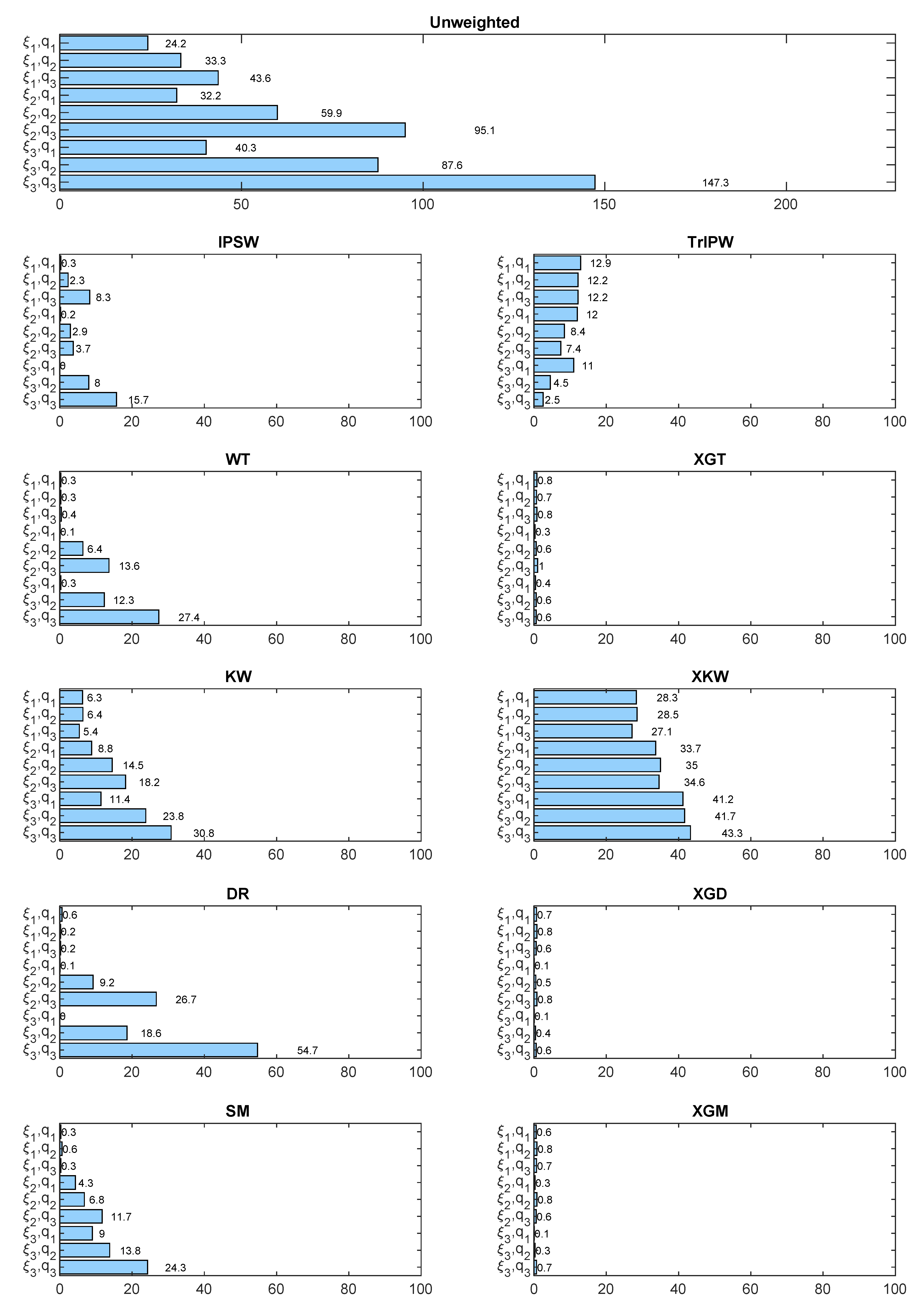
The estimators considered are: the unweighted sample mean ($\widehat{\overline{Y}}$), IPSW with logistic regression (${\widehat{\overline{Y}}}_{IPSW}$), Tree-Based Inverse Propensity Weighted estimation(${\widehat{\overline{Y}}}_{TrIPW}$), Kernel Weighting (${\widehat{\overline{Y}}}_{KW}$), Matching with linear regression (${\widehat{\overline{Y}}}_{SM}$), Doubly Robust with linear regression for Matching and logistic regression for PSA (${\widehat{\overline{Y}}}_{DR}$), Training with linear regression for Matching and logistic regression for PSA (${\widehat{\overline{Y}}}_{WT}$), XGBoosted kernel weighting (${\widehat{\overline{Y}}}_{XKW}$), Matching with XGBoost (${\widehat{\overline{Y}}}_{XGM}$), Doubly Robust with linear regression for PSA and XGBoost for Matching (${\widehat{\overline{Y}}}_{XGD}$) and Training with linear regression for PSA and XGBoost for Matching (${\widehat{\overline{Y}}}_{XGT}$). For those using XGBoost, only its default hyperparameters are considered in this simulation.

The results for every possible population/propensities combination, with different values of the correlation coefficient $\rho$, can be consulted in Figure 1, Figure 2, Figure 3, Figure 4, Figure 5 and Figure 6.

Models ${\xi }_1$ and $q_1$ are linear models. Therefore, linear/logistic regression is theoretically unbeatable for those models. However, it can be observed that XGBoost can also effectively remove the bias in those cases. The difficulties of linear/logistic regression arise as the non-linearity of the models is increased. XGBoost is, however, still able to learn the model in those scenarios. The decrease in bias and MSE of the XGBoost technique with respect to linear/logistic regression is very noticeable in the case of the ${\xi }_3$ and $q_3$ model, and it is observed how this good behavior is accentuated as the correlation between the variables increases.

That is not the case for the ${\widehat{\overline{Y}}}_{TrIPW}$ or ${\widehat{\overline{Y}}}_{XKW}$ estimators. They seem to be suffering from overfitting [40]. Further analysis from simulations considering real populations and hyperparameter optimization will determine if their performance can be fixed.

Regarding doubly robust estimators, again the high learning capacity of Matching with XGBoost causes that combining it with PSA does not necessarily improves the results. In practice, the complexity of real data models may change that fact.

4.2. Real Populations

Following the experiment described in the previous section, the study is repeated with real populations. The same estimators are considered. Default XGBoost hyperparameters are used for an initial simulation. The relative bias is kept as a metric but the mean squared error is replaced by the relative rooted mean squared error ($\%RRMSE$) in order to obtain comparable results.

$$\begin{array}{c}\hfill \%RRMSE=\sqrt{\frac{1}{B}\sum _{b=1}^B{\left({\widehat{\mu }}^{\left(b\right)}-{\mu }_y\right)}^2}/{\mu }_y\times 100\end{array}$$

(36)

Two datasets are used following two different sampling strategies for each one. In each simulation run, three possibilities for sample sizes, $n_V=n_R=1000$, $n_V=n_R=2000$ and $n_V=n_R=5000$, are considered.

The first population, denoted as P1, corresponds to the Hotel Booking Demand Dataset [48]. It includes the data of bookings for a resort hotel and a city hotel due to arrive between the 1 July 2015 and 31 August 2017. In total, it has 119,390 bookings of which 34% are from the resort hotel and 66% from the city hotel. For the first nonprobability sampling strategy, denoted as S1, resort bookings have 10 times more probability of being chosen than city bookings. For the second nonprobability sampling strategy, denoted as S2, city bookings have five times more probability of being chosen than resort bookings. The target variable is the mean number of weeknights (Friday included) which are booked. In order to estimate it, a probability sample $s_R$ is also obtained via a simple random sampling. The remaining variables included in the dataset are used as covariates, excluding the reservation status and the reservation status date, with a total of 28 covariates.

The second population, denoted as P2, is the Adult Dataset [49]. It includes census income information for 32,561 adult individuals from the 1994 Census database of the United States. For the first nonprobability sampling strategy, denoted as S1, individuals who make over $50K a year have double the probability of being chosen. For the second nonprobability sampling strategy, denoted as S2, individuals who make over $50K per year have a propensity to participate multiplied by $Pr\left(a\right)=2a^2$, where a is the individual’s age. The target is estimating the proportion of individuals who make over $50K per year. Therefore, in this case, the target variable in the dataset is binary instead of continuous. Also, in this scenario, the propensities depend on the target variable itself and this dependance may not even be linear. Every other variable in the dataset is used as covariate, for a total of 14 covariates. The probabilistic samples are obtained via simple random sampling.

The bias and relative rooted mean squared error results for each case with each estimator can be viewed in

Table 1. Relative bias (%) for each real population case.

	$\widehat{\overline{\mathit{Y}}}$	${\widehat{\overline{\mathit{Y}}}}_{\mathit{IPSW}}$	${\widehat{\overline{\mathit{Y}}}}_{\mathit{TrIPW}}$	${\widehat{\overline{\mathit{Y}}}}_{\mathit{KW}}$	${\widehat{\overline{\mathit{Y}}}}_{\mathit{SM}}$	${\widehat{\overline{\mathit{Y}}}}_{\mathit{DR}}$	${\widehat{\overline{\mathit{Y}}}}_{\mathit{WT}}$	${\widehat{\overline{\mathit{Y}}}}_{\mathit{XKW}}$	${\widehat{\overline{\mathit{Y}}}}_{\mathit{XGM}}$	${\widehat{\overline{\mathit{Y}}}}_{\mathit{XGD}}$	${\widehat{\overline{\mathit{Y}}}}_{\mathbf{XGT}}$
P1S1 1000	18.9	5.5	11.1	3.7	4.5	4.6	4.5	0.2	3.5	3.5	3.3
P1S1 2000	18.9	5.5	10.9	4	4.9	4.9	4.8	−11.9	2.8	2.8	2.5
P1S1 5000	18.6	4.6	10.1	4.2	4.8	4.8	4.7	−7.5	2.2	2	1.7
P1S2 1000	−9.2	−4.1	−5.4	−2.1	−5	−4.1	−4.1	−13.4	−2.6	−2.5	−2.5
P1S2 2000	−9.2	−4.2	−5.5	−2	−4.9	−4.1	−3.9	−7.5	−1.9	−1.8	−1.8
P1S2 5000	−9.1	−3.9	−5.2	−2.4	−4.7	−3.8	−3.6	1.4	−1.4	−1.3	−1.3
P2S1 1000	60	34.4	37	33.5	33.2	33.2	30	8.9	25.9	25.8	24.8
P2S1 2000	58.7	33.3	36	33.1	30.8	30.5	29.2	−12	25	24.7	24
P2S1 5000	54.8	31.3	33.7	30.7	31.1	27.9	27.6	−11.8	23.4	23.2	22.8
P2S2 1000	78.3	34.8	39.8	33	34.9	33.8	31	−5.6	26.4	25.9	24.4
P2S2 2000	76.5	33.9	39.1	32.4	32.2	31.2	30.2	−31.1	25	24.9	23.6
P2S2 5000	71.1	31.7	36.6	30.3	30.6	28.5	28.2	−19.4	23.3	23	22.4

and

Table 2. Relative RMSE (%) for each real population case.

	$\widehat{\overline{\mathit{Y}}}$	${\widehat{\overline{\mathit{Y}}}}_{\mathit{IPSW}}$	${\widehat{\overline{\mathit{Y}}}}_{\mathit{TrIPW}}$	${\widehat{\overline{\mathit{Y}}}}_{\mathit{KW}}$	${\widehat{\overline{\mathit{Y}}}}_{\mathit{SM}}$	${\widehat{\overline{\mathit{Y}}}}_{\mathit{DR}}$	${\widehat{\overline{\mathit{Y}}}}_{\mathit{WT}}$	${\widehat{\overline{\mathit{Y}}}}_{\mathit{XKW}}$	${\widehat{\overline{\mathit{Y}}}}_{\mathit{XGM}}$	${\widehat{\overline{\mathit{Y}}}}_{\mathit{XGD}}$	${\widehat{\overline{\mathit{Y}}}}_{\mathbf{XGT}}$
P1S1 1000	19.1	6.3	11.7	5.4	5.6	5.5	5.4	17.4	4.7	4.7	4.6
P1S1 2000	18.9	5.9	11.2	4.9	5.4	5.3	5.3	20.6	3.6	3.6	3.4
P1S1 5000	18.7	8.6	10.3	4.4	5	5.6	4.9	8.8	2.5	2.5	2.2
P1S2 1000	9.5	5.7	5.9	5.9	5.9	5.3	5	20	3.9	3.9	3.9
P1S2 2000	9.3	4.8	6	4.2	5.3	4.7	4.4	19.5	2.8	2.7	2.7
P1S2 5000	9.2	4.2	5.4	3	4.8	4	3.8	11	1.9	1.8	1.8
P2S1 1000	60.3	35	37.6	34.2	33.8	33.9	30.7	77	26.9	26.7	25.7
P2S1 2000	58.9	33.5	36.3	33.4	31.1	30.8	29.5	39.6	25.4	25.1	24.4
P2S1 5000	54.9	31.4	33.8	30.9	31.8	28	27.7	15.8	23.5	23.3	22.9
P2S2 1000	78.5	35.4	40.4	33.7	35.4	34.3	31.6	69.4	27.2	26.8	25.3
P2S2 2000	76.6	34.2	39.4	32.7	32.5	31.5	30.5	40.2	25.4	25.4	24.1
P2S2 5000	71.1	31.8	36.7	30.4	30.9	28.7	28.3	20	23.5	23.2	22.6

respectively.

Again, as it happened with the simulated data, a significant improvement in the estimations can be observed when using XGBoost instead of linear or single tree regressors. This improvement is more relevant now since the datasets are more complex and closer to real scenarios. The results are also better, as more data is avaliable. In the majority of cases, the Matching based variants obtain the best results. However, for some specific cases, XGBoosted Kernel Weighting is better. This probably happens where the algorithm is not overlearning. This assumption is confirmed by later simulations considering hyperparameter optimization in which the methods always behave reliably.

Regarding doubly robust estimators, combining SM with PSA may yield slightly more accurate estimations in these cases with XGBoost as well. This improvement can be more noticeable if a more direct approach like ${\widehat{\overline{Y}}}_{XGT}$ is applied instead of a basic combination like ${\widehat{\overline{Y}}}_{XGD}$.

Some of these results may be improved by applying variable selection, specifically those using linear of logistic regression. Tree based algorithms like XGBoost or CART apply variable selection internally by themselves.

Finally, as explained in Section 3.1, hyperparameter optimization is also considered via the Tree-structured Parzen Estimator (TPE) algorithm [45], as implemented in the software package Optuna [50]. The TPE algorithm is able to quickly discard inappropiate settings, so a wide search space may be specified. We have run simulations for the boosted matching estimator ${\widehat{\overline{Y}}}_{XGM}$ and for the XGBoosted kernel weighting estimator ${\widehat{\overline{Y}}}_{XKW}$. The sample size for this scenario is 1000 since it is the hardest case. Each hyperparameter set evaluated by the algorithm is validated measuring its Mean Squared Error among 50 sub-simulations. Once the best values for each specific case are selected with this procedure, they are used for a new simulation in the same conditions as the one without optimization. Every real population and sampling strategy is considered.

The results can be observed in

Table 3. Relative bias (%) for each optimized case.

		Non Optimized		Optimized
	$\widehat{\overline{\mathit{Y}}}$	${\widehat{\overline{\mathit{Y}}}}_{\mathit{XKW}}$	${\widehat{\overline{\mathit{Y}}}}_{\mathit{XGM}}$	${\widehat{\overline{\mathit{Y}}}}_{\mathit{XKW}}$	${\widehat{\overline{\mathit{Y}}}}_{\mathit{XGM}}$
P1S1 1000	18.9	0.2	3.5	0.4	1.2
P1S2 1000	−9.2	−13.4	−2.6	−1.1	−1.5
P2S1 1000	60.0	8.9	25.9	5.2	25.1
P2S2 1000	78.3	−5.6	26.4	2.0	25.5

and

Table 4. Relative RMSE (%) for each optimized case.

		Non Optimized		Optimized
	$\widehat{\overline{\mathit{Y}}}$	${\widehat{\overline{\mathit{Y}}}}_{\mathit{XKW}}$	${\widehat{\overline{\mathit{Y}}}}_{\mathit{XGM}}$	${\widehat{\overline{\mathit{Y}}}}_{\mathit{XKW}}$	${\widehat{\overline{\mathit{Y}}}}_{\mathit{XGM}}$
P1S1 1000	19.1	17.4	4.7	4.0	3.2
P1S2 1000	9.5	20.0	3.9	4.1	3.4
P2S1 1000	60.3	77.0	26.9	10.6	26.2
P2S2 1000	78.5	69.4	27.2	7.8	26.5

. The optimization considerably improves the estimations. In some cases, this improvement is so significant that the method which was the worst one without optimization is now the best alternative. Therefore, the importance of applying this kind of procedure is confirmed in order to obtain reliable results, especially for those estimators that have shown to suffer greatly from overlearning.

5. Application to a Survey on Social Effects of COVID-19 in Spain

This section illustrates the estimation procedures that we have empirically described in a web survey in which respondents were selected by targeting Internet ads at specific profiles.

ESPACOV [51] is a survey that was conducted in Spain in the fourth week of the strict lockdown imposed on 14 March 2020, and provides information on the living conditions of the population, acquired habits, health and consequences of the state of alarm and home confinement. ESPACOV was run by the Institute for Advanced Social Studies (IESA) and the sample was collected via paid advertisements on Google Ads and Facebook/Instagram (nonprobability sampling). A total of 1881 interviews were completed.

Table 5. Obtained sample distributions by sex and age group and by education level, and comparison with population parameters.

	ESPACOV Sample	Spanish Population
Age group
Men
18–29	9.7	7.6
30–44	9.3	12.9
45–64	11.3	17.6
65+	16.1	10.3
Women
18–29	10.6	7.3
30–44	13.7	12.9
45–64	17.9	17.9
65+	11.6	13.5
Education
Obligatory or less	16.2	45.6
Secondary	33.8	21.7
Tertiary	49.6	32.7

compares unweighted sample distributions by age group and sex and by education level with Spanish population data [52,53].

Due to coverage and participation bias, people with tertiary education are over-represented, and less educated people vastly under-represented. There are also representation issues in the different age groups for each sex.

We have considered the April 2020 Barometer of the Spanish Center for Sociological Research [54] as the source of auxiliary information. The barometers are probability surveys carried out on a monthly basis, and their main objective is to measure Spanish public opinion at that time. They involve interviews with approximately 2500 randomly-chosen people from all over the country, with extensive social and demographic information on them being gathered for analysis as well as their opinions. The survey follows a multi-stage, stratified cluster sampling, with selection of the primary sampling units (municipalities) and of the secondary units (census sections) randomly with proportional allocation, and of the last units (individuals) by random routes and sex and age quotas. The barometer dataset is often viewed as a reliable source of official statistics and contains a number of common variables with the ESPACOV dataset. More precisely, these include gender, age, province, municipality size, education level, working status and self-positioning in the ideological scale (10-point Likert, where 1 represents “far left” and 10 “far right”).

We apply the proposed methods to estimate the population mean of the variable “Rate the government action to control the pandemic, from 0 to 10”. The values of the estimators ${\widehat{\overline{Y}}}_{IPSW}$, ${\widehat{\overline{Y}}}_{TrIPW}$, ${\widehat{\overline{Y}}}_{KW}$, ${\widehat{\overline{Y}}}_{SM}$, ${\widehat{\overline{Y}}}_{DR}$, ${\widehat{\overline{Y}}}_{WT}$, ${\widehat{\overline{Y}}}_{XKW}$, ${\widehat{\overline{Y}}}_{XGM}$, ${\widehat{\overline{Y}}}_{XGD}$ and ${\widehat{\overline{Y}}}_{XGT}$ are computed for each variable. The unadjusted simple sample mean $\widehat{\overline{Y}}$ from the nonprobability sample is also included. Results from using the common set of covariates which are available in both datasets are presented in

Table 6. Estimates of the population mean of the variable measuring the rating (1–10) of the Spanish government action to control the COVID-19 pandemic.

Estimator	Mean	S. Deviation
$\widehat{\overline{Y}}$	5.52	0.08
${\widehat{\overline{Y}}}_{IPSW}$	5.04	0.10
${\widehat{\overline{Y}}}_{TrIPW}$	5.13	0.09
${\widehat{\overline{Y}}}_{KW}$	4.95	0.12
${\widehat{\overline{Y}}}_{SM}$	5.18	0.09
${\widehat{\overline{Y}}}_{DR}$	5.21	0.09
${\widehat{\overline{Y}}}_{WT}$	5.38	0.09
${\widehat{\overline{Y}}}_{XKW}$	5.33	0.72
${\widehat{\overline{Y}}}_{XGM}$	4.91	0.10
${\widehat{\overline{Y}}}_{XGD}$	4.92	0.10
${\widehat{\overline{Y}}}_{XGT}$	4.89	0.09

.

The results generally show that the application of bias correction techniques provides an important shift (towards a lower mean rate) with respect to the unweighted estimate, especially for those which were the most reliable ones during the simulations (${\widehat{\overline{Y}}}_{XGM}$, ${\widehat{\overline{Y}}}_{XGD}$ and ${\widehat{\overline{Y}}}_{XGT}$). Standard deviations were estimated via bootstraping [44]. 2000 resamples with replacement are obtained in order to calculate the deviation for each method. They show a small and expectable increase in variance from the unweighted case except for the ${\widehat{\overline{Y}}}_{XKW}$ estimator. As seen in the simulations, this behavior is to be expected and should be solved via hyperparameter tuning.

However, the chosen variable is closely related to the ideological scale covariate. We also apply the methods to estimate the population means of the variables, rating, from 1 to 5, the confidence in the following groups/institutions to manage the current health crisis: health workers, the armed forces, the police, the Spanish government and scientists. The results are presented in

Table 7. Estimates of the population means of the variables measuring the rating (1–5) of the confidence in different groups/institutions to manage the current health crisis.

Variable	$\widehat{\overline{\mathit{Y}}}$	${\widehat{\overline{\mathit{Y}}}}_{\mathit{IPSW}}$	${\widehat{\overline{\mathit{Y}}}}_{\mathit{TrIPW}}$	${\widehat{\overline{\mathit{Y}}}}_{\mathit{KW}}$	${\widehat{\overline{\mathit{Y}}}}_{\mathit{SM}}$	${\widehat{\overline{\mathit{Y}}}}_{\mathit{DR}}$	${\widehat{\overline{\mathit{Y}}}}_{\mathit{WT}}$	${\widehat{\overline{\mathit{Y}}}}_{\mathit{XKW}}$	${\widehat{\overline{\mathit{Y}}}}_{\mathit{XGM}}$	${\widehat{\overline{\mathit{Y}}}}_{\mathit{XGD}}$	${\widehat{\overline{\mathit{Y}}}}_{\mathit{XGT}}$
Health workers	4.48	4.41	4.45	4.4	4.45	4.43	4.43	4.39	4.44	4.43	4.44
Armed forces	4.01	3.99	4.12	3.99	3.99	3.97	3.92	4.1	4.03	4.03	4.03
Police	4.04	4.05	4.14	4.07	4.05	4.04	4	3.92	4.07	4.07	4.04
Spanish government	2.94	2.7	2.77	2.68	2.76	2.78	2.87	2.55	2.61	2.62	2.62
Scientists	4.18	4.12	4.11	4.1	4.13	4.14	4.18	3.95	4.03	4.03	4.04

. They show that the differences are not as significant when the target variables are not related to the covariates used.

6. Conclusions

A long and ongoing literature is concerned with the evaluation of selection bias in web surveys. Propensity scorse and matching estimators based on linear models are the established workhorses in this literature. The emerging literature in statistical learning might help to increase the precision of the estimates obtained by these methods.

Although machine learning methods have many well-documented advantages in prediction and classification, it is not obvious that using them for propensity scores and matching estimation in a nonprobability framework will reduce the bias in the estimation of parameters. In this work we present four different methods to estimate parameters based on the use of an important ML technique, the XGBoots method, to predict the values of the target variable in the probability sample and also to determine the propensities of participating in the nonprobability sample.

Our work contributes to the literature in evaluating the performance of classical and machine learning based PSA estimators, matching estimators as well as other methods of estimation from web survey data that are more innovative.

To be as close as possible to other recent estimation works in nonprobability surveys, we have replicated the experiment carried out by [47]. When comparing results from both simulations, we observe that estimators involving XGBoost provide better results overall in certain non-linear situations in comparison to the case where linear models are used. These results are relevant considering that, in practice, models will rarely be linear. In fact, they will likely be much more complex than the ones considered in this simulation. For this reason, we compare the different estimators in two real datasets. We compared performance of XGBoost to a classical regression approach, with the former providing good results in terms of bias and Mean Square Error reduction.

Our findings are mixed. Our evidence suggests the usage of XGBoost is more powerful at removing selection bias in nonprobability samples than traditional linear regression models in scenarios where the propensity model is not linear and the auxiliary variables used for adjustments are related to both the propensity and the variable of interest. In addition, the simulations also show the efficiency of the use of recent training techniques like [34,39] compared to the alternatives of PSA, matching, and double robust [32] techniques.

However, these results can also be unreliable when the algorithms suffer from overfitting. Hyperparameter optimization has shown to be highly effective at controlling this issue. These kind of procedures are therefore important when producing estimations. We will look further into this matter in future works.

The proposed method is also used to analyze a nonprobability survey sample on the social effects of COVID-19. The results of this application show that selection bias correction techniques have the potential to provide substantial changes in the estimates of population means in nonprobability samples.

In conclusion, the improved learning capacity of XGBoost is capable of significantly reducing bias and MSE in certain scenarios according to our simulations, but it is important to explore its limits with real use cases. Generally speaking, our results illustrate several methods to do inference with nonprobability samples and highlight the importance and usefulness of auxiliary information from probability survey samples. Propensity Score Adjustment and model-based methods are recommended when the sample can be subject to strong selection bias. XGBoost can yield more accurate predictions when the data behavior is more complex, which typically occurs in situations with high dimensionality. Those are the scenarios where we could particularly benefit the most from Xgboost, although it is suitable for most of the situations.