Modeling the Context of the Problem Domain of Time Series with Type-2 Fuzzy Sets

Abstract

Data analysis in the context of the features of the problem domain and the dynamics of processes are significant in various industries. Uncertainty modeling based on fuzzy logic allows building approximators for solving a large class of problems. In some cases, type-2 fuzzy sets in the model are used. The article describes constructing fuzzy time series models of the analyzed processes within the context of the problem domain. An algorithm for fuzzy modeling of the time series was developed. A new time series forecasting scheme is proposed. An illustrative example of the time series modeling is presented. The benefits of contextual modeling are demonstrated.

1. Intro

The activity of any modern organization is associated with the timely adoption of urgent management decisions [1]. This is required to evaluate the states of some complex systems. The decision-maker (DM) requires knowledge of the specifics of the problem domain and the ability to use various tools for data analysis and working with existing knowledge. This process forms the requirements for data analysis methods. Methods should work in some contexts of analyzed object behavior. Methods consider features and limitations of analyzed objects. The same dataset in different subject areas can have different interpretations and analysis results.

The analysis of a set of the time series in [2,3] for process detection is used. The intelligent process analysis described by the authors does not apply knowledge about the correlation between objects of a problem area. The process analyses with intelligent methods in these works do not consider the features of the problem domain. The process detection quality improvement needs more complex models than quantitative indicators by a time series model.

Currently, a large number of works describe various approaches to the application of context in data mining [4,5,6,7,8,9]. The use of context will improve the quality and efficiency of data analysis presented by time series.

In the works considered, the context is formed based on ontologies. Ontologies are used for:

• Increasing the interoperability of data processing systems represented by THE time series due to data unification based on ontological representations [4];
• Improving the accuracy of search engine requests in predictive analytics [5];
• Associations of the time series with messages in social networks, considering the specifics of the problem domain: company structure, names of employees, etc. [6];
• The transition from numerical data to semantic fragments of the neural network structure [7];
• Detecting changes in a group of related time series [9].

Modeling various processes and systems under uncertainty has many practical applications. Traditionally, time series models are used to model dynamics. These models allow reflecting the history of changes in process indicators. A time-series basis is a specific approach for analyzing numerical data, unlike, for example, classical statistical methods. Time series models allow reflecting the dependence of a sequence of the time series point values on points at previous moments. The problem is that the values of the indicators represented by a time series in complex systems can contain a cumulative assessment of the influence of several factors. The problem lies in improving the accuracy of the approximation of the modeled system based on time series models with uncertainty, noise, and insufficient data. Fuzzy time series models allow us to extract easily understandable rules for a researcher to perceive from historical data for analysis and forecasting tasks. However, several problems are still relevant to the solution. Time series modeling is often based only on the history of the data itself. That condition does not allow identifying the correct patterns, limitations, and features of the modeled processes. The main objects for building an accurate model of the analyzed process involve the information about changes in the indicators and the conditions of the solved problem. In other words, the analysis of the number sequence of different real-world objects may have different results [10,11]. The conditions of this modeling are called contextual modeling of the time series. Time series models, built based on type-2 fuzzy sets, can have more modeling uncertainty benefits. Their advantages are:

• The ability to model the uncertainty of the choice of antecedents and consequents in the rules;
• The ability to select the parameters of type-1 membership functions;
• A reduction in the number of type-1 fuzzy labels while maintaining the quality of the time series approximation.

The task of the modeling context is closely related to granular computing. The common factor is that the modeling result is problem-oriented. The theory of granular computations to the time series analysis in the works by [12,13,14] is considered. Information granules presented by sets of fuzzy tendencies of the time series can make time series context modeling:

$$G=\{T,D,I\},$$

(1)

where

T—the direction of tendency;

D—linguistic value of duration;

I—linguistic value of intensity.

The choice of fuzzy tendencies for modeling information granules is because they contain information about the dynamics of the time series. In this case, the novelty is the use of type-2 fuzzy sets for information granule construction and the creation of rules set about the patterns of behavior of the time series. The second feature is that the model includes the context of the problem domain, which defines the conditions for modeling the time series.

Improving the quality of the time series modeling and forecasting by using only the history of changes has a natural limitation: it is impossible to create an immutable and accurate time-series mathematical model without using an object’s knowledge. We propose to append the time series model with fuzzy rules for adapting the base mathematical model (or a set of models) to the changing external conditions of the object’s functioning, which affect the changes in indicators.

Thus, context analysis means the models use additional information about the various conditions of the functioning of a given model to reduce the dimension of the analyzed data and increase the accuracy of modeling.

2. Related Work

The possibility of an integral representation of knowledge about the object behavior and its uncertainty is the main advantage of modeling information granules. The process of obtaining and presenting information granules is hierarchical and multi-stage [15]. Information granule modeling is a multidisciplinary process. Such modeling opens up opportunities for creating intelligent systems with the interpretation of modeling results [13]. In decision making, the problem domain can have different degrees of uncertainty: uncertainty in the input data, uncertainty in the principles of control, insufficient input data, noise in data, etc. Including expert knowledge about the processes is not always objectively accurate. The papers [16,17,18,19,20] discuss various methods to overcome these problems: decision trees, clustering, deep learning methods, ontological engineering, fuzzy logic, time series models, etc.

In decision-making systems, it is often necessary to analyze data with time variability. This increases the complication of the analysis due to the growing amount of data and the complication of the applied models. In some research works on dynamic data analysis, time series models with information granules have been used. The works [14,21] show that time series forecasting and reducing the data dimensions can be made by information granule modeling. The authors consider the approach of [22], based on type-2 fuzzy sets for justified granularity. Granules are created by a balance between their experimental rationale and semantics. The work [23] discusses the entropy approach for interval discretization of information granules when predicting prices in the stock exchange. The conclusion is that granular computing is a method of generalization in knowledge representation and as a basis for various modeling tools. Non-linear dependencies can be more accurately represented in information granule models in comparison to interval models [24].

Work [25] discusses the context concept in information retrieval, considering context as an extension of local information about the object under study with some global information. In the article [26], the citation context helps to rank the scientific publication citations’ importance and gives additional information used by machine learning models. In [27], this context helps to improve the accuracy of local methods for detecting objects in images. In this work, the context promotes obtaining information about related objects with the analyzed one.

Large volumes of data in the databases of information systems are a great source for analysis behavior on complex organizational and technical systems. Using such information for process identification is important for management [28].

Time series models can represent uncertainty by value or by time. The following approaches in works [12,29,30] was described:

• Fuzzy Transform (F-transform) [29,30] is a soft computing approximation technique. The advantages of the F-transform in various applications are demonstrated, such as time series analysis and approximation, image compression, anomaly detection.
• Time series fuzzification by time in [12] is described.

The use of high-order fuzzy sets helps to model the uncertainty of various real-world objects. The work [31] shows that uncertainty can be divided into random (inaccuracies in the processing of statistical signals) and linguistic (inaccuracies in the expert statements).

The hybridization of the time series modeling approaches allows the creation of intellectual methods for data processing and analysis for decision-making systems.

3. Time Series Model

A model of discrete numerical time series is created with preliminary fuzzification by type-2 fuzzy sets. This approach helps to simplify the procedure for forming a rule base for fuzzy inference when analyzing time series. The problem of determining the boundaries of intervals of type-2 fuzzy sets lies in solving them. The time series model considers the context of the problem domain with the conditions and the nature of its main tendencies. A triangular form of fuzzy sets is used due to the small computational complexity.

A discrete numerical time series is given as:

$$ts=\left\{t{s}_t\right\},t\in [0,l],t\in \mathbb{N}$$

(2)

where $t{s}_t$—time series value at a time point t; l—length of the time series. At each moment $t>0$, the value of the tendency of the time series can be determined:

$$Ten{d}_t=t{s}_t-t{s}_{t-1},$$

(3)

where $Ten{d}_t$—a numerical representation of the direction and intensity of the tendency of a time series at a point in time t; $t{s}_t,t{s}_{t-1}$—time series values at moment t and $t-1$, respectively.

For fuzzy modeling of the time series tendencies, a universe of type-2 fuzzy sets is defined as: $U={\tilde{A}}_i$, and $i\in \mathbb{N}$ is the number of fuzzy sets in the universe.

Type-2 fuzzy sets can be represented as:

$$\tilde{A}=((x,u),{\mu }_{\tilde{A}}(x,u))|\forall x\in U^x,\forall u\in J_x\subseteq [0,1]$$

(4)

where $x\in U^x$ and $u\in J_x\subseteq [0,1]$ in which $0\le {\mu }_{\tilde{A}}(x,u)\le 1$, $J_x$ is the range of values of the function $\mu (x)$. x—is a crisp time series value, and $U^x$—is a universe of the time series values.

Lower membership function $\tilde{A}$ is called the function ${\underline{\mu }}_A:U^x\to [0,1]$ and defined as ${\underline{\mu }}_A(x)=\inf J_x,x\in U^x$.

Upper membership function $\tilde{A}$ is called the function ${\overline{\mu }}_A:U^x\to [0,1]$ and defined as ${\overline{\mu }}_A(x)=\sup J_x,x\in U^x$.

Type-2 fuzzy set $\tilde{A}$ will be interval if ${\mu }_A(x,u)=1\forall x\in U^x,u\in J_x$.

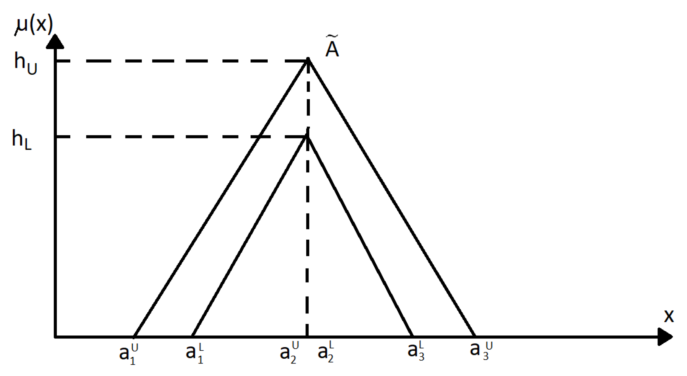
Time series modeling needs to define interval fuzzy sets and their shape. Figure 1 shows the appearance of the sets.

Triangular fuzzy sets are defined as follows:

$${\tilde{A}}_i=({\tilde{A}}_i^U,{\tilde{A}}_i^L)=((a_{i1}^u,a_{i2}^u,a_{i3}^u,h({\tilde{A}}_i^U)),(a_{i1}^l,a_{i2}^l,a_{i3}^l,h({\tilde{A}}_i^l))).$$

(5)

where ${\tilde{A}}_i^U$ and ${\tilde{A}}_i^L$ are triangular type-1 fuzzy sets, $a_{i1}^u,a_{i2}^u,a_{i3}^u,a_{i1}^l,a_{i2}^l,a_{i3}^l$ are reference points of type-2 interval fuzzy set ${\tilde{A}}_i$, and h is the maximum value of the membership function of the element $a_i$ (for the upper and lower membership functions, respectively), means that $(\stackrel{A}{˜}{)}_i$ depends of height of triangle.

An operation of combining fuzzy sets of type 2 is required when working with a rule base based on the values of a time series. The combined operation is defined as follows:

$$\begin{array}{c}{\tilde{A}}_1\oplus {\tilde{A}}_2=({\tilde{A}}_1^U,{\tilde{A}}_1^L)\oplus ({\tilde{A}}_2^U,{\tilde{A}}_2^L)\\ =((a_{11}^u+a_{21}^u,a_{12}^u+a_{22}^u,a_{13}^u+a_{23}^u;\\ min(h_1({\tilde{A}}_1^U),h_1({\tilde{A}}_2^U))),min(h_2({\tilde{A}}_1^U),h_2({\tilde{A}}_2^U)));\\ (a_{11}^l+a_{21}^l,a_{12}^l+a_{22}^l,a_{13}^l+a_{23}^l;\\ min(h_1({\tilde{A}}_1^L),h_1({\tilde{A}}_2^L)),min(h_2({\tilde{A}}_1^L),h_2({\tilde{A}}_2^L)));\end{array}$$

Proposition 1.

A fuzzy time series model, reflecting the context of the problem domain, will be described by two sets of type-2 fuzzy labels:

$$\widetilde{ts}=(\tilde{A},{\tilde{A}}^C),$$

(6)

where $\tilde{A}$—a set of type-2 fuzzy sets describing the tendencies of the time series obtained from the analysis of the points of the time series, $|\tilde{A}|=l-1$; ${\tilde{A}}^C$—a set of type-2 fuzzy sets describing the trends of the time series obtained from the context of the problem domain of the time series, $|{\tilde{A}}^C|<<l-1$.

The component $\tilde{A}$ of model (6) is extracted from time series values by fuzzifying all numerical representations of the time series tendencies. By the representation of information granules in the form of fuzzy tendencies of the time series (1), the numerical values of the tendencies are fuzzified: $\widetilde{A_t}=\mu (Ten{d}_t)=\mu (t{s}_t-t{s}_{t-1}),t>0$.

The component ${\tilde{A}}^C$ of model (6) by expert or analytical methods is formed and describes the most general behavior of the time series. This component is necessary for solving problems:

• Justification of the choice of the boundaries of the type-2 fuzzy set intervals when modeling a time series.
• Analysis and forecasting of a time series with a lack of data or when they are noisy.

Thus, the time series context, represented by the component ${\tilde{A}}^C$ of model (6), is determined by the following parameters:

• Rate of tendency change ${\widetilde{A_t}}^C$.
• Number of tendency changes $|{\tilde{A}}^C|$.

4. Modeling Algorithm

The modeling procedure contains the following steps:

• Check the constraints of the time series: discreteness; length being more than two values.
• Calculate the tendencies $Ten{d}_t$ of the time series by (3) at each moment $t>0$.
• Determine the universe for the fuzzy values of the time series tendencies: $U={\tilde{A}}_i,i\in \mathbb{N}$ is the number of fuzzy sets in the universe. Type-2 fuzzy sets $\tilde{A}$ are given by membership functions of a triangular form, and at the second level, they are intervals; see Figure 1.
• By an expert or analytical method, obtain the rules from the time series as a set of pairs of type-2 fuzzy sets: $Rule{s}^C=\left\{R_r^C\right\},r\in \mathbb{N}$, where $R_r^C$ is a pair $({\tilde{A}}_i^C,{\tilde{A}}_k^C)$, ${\tilde{A}}_i^C$ is the antecedent of the rules, ${\tilde{A}}_k^C$ is the consequent of the rules and $i,k$ are the indices specifying the relation of the consecutive in time of the antecedent and the consequent, $i<k<=l$.
• Fuzzify the time series tendencies $\tilde{A}=\left\{\widetilde{A_t}\right\}=\left\{\mu (t{s}_t-t{s}_{t-1})\right\}\forall t\in [0,\dots ,l]$ and create a rule base: $Rules=\left\{R_r^C\right\},r\in \mathbb{N}$, where $R_k$ is a pair $({\tilde{A}}_i,{\tilde{A}}_k)$, $\widetilde{A_i}$ is the antecedent of the rules, $\widetilde{A_k}$ is the consequent of the rules and $i,k$ are the indices specifying the relation of the consecutive in time of the antecedent and the consequent, $i<k<=l$.
• Merge the rule base with rules derived from the context: $Rules\cup Rule{s}^C$.
• Correct the fuzzy sets extracted from the time series along the context boundaries of the intervals of type-2 fuzzy sets:

  $$\begin{array}{c}\hfill inf(\widetilde{A_t})=max(inf({\tilde{A}}_t),inf({\tilde{A}}_t^C))\\ \hfill sup(\widetilde{A_t})=min(sup({\tilde{A}}_t),sup({\tilde{A}}_t^C))\end{array}$$

  (7)
• Apply the resulting rule base for fuzzy inference when modeling and predicting time series values.

5. Time Series Forecasting with Using of Context

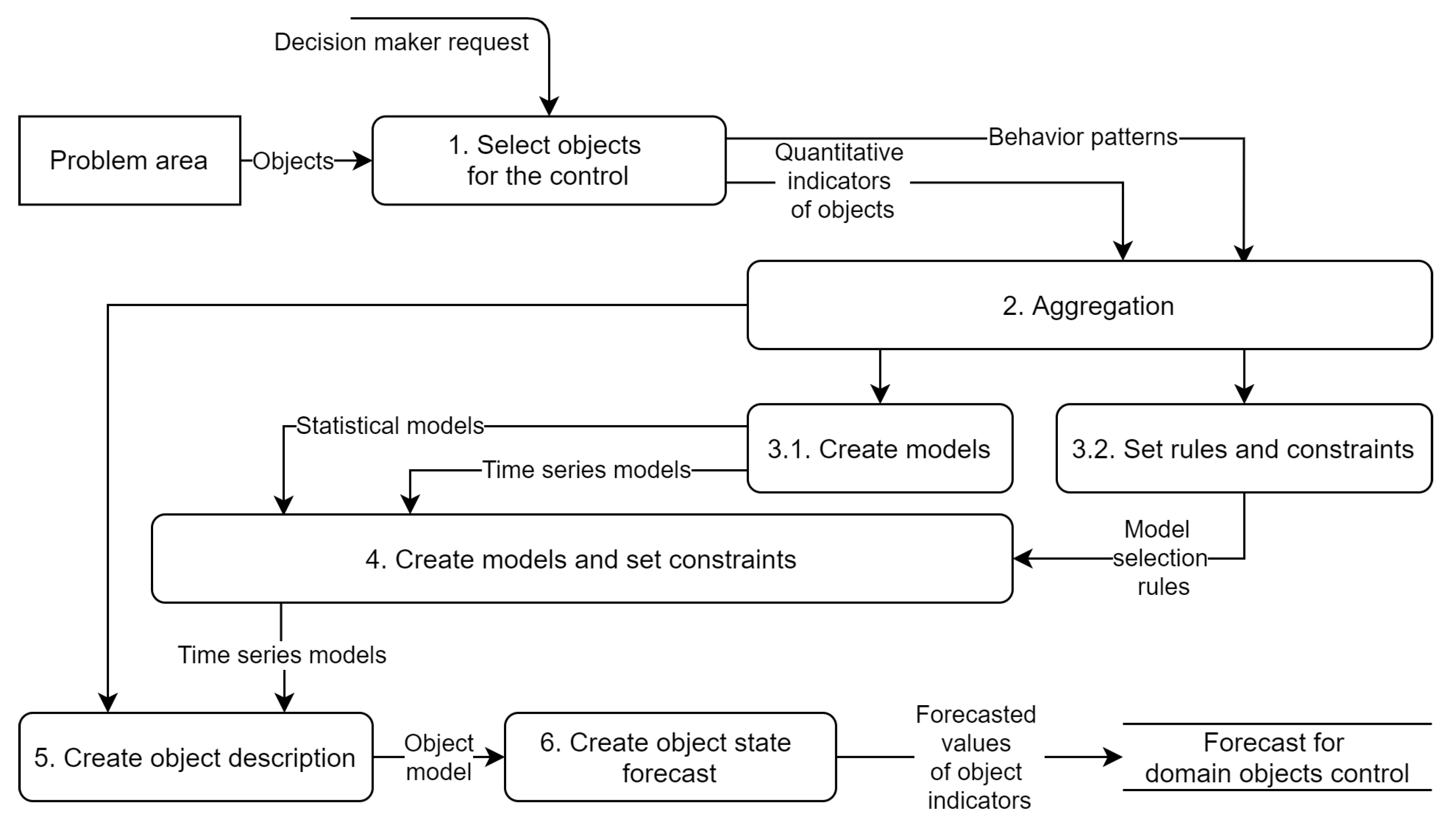
The analysis of dynamic data using the context can be presented by the following scheme, Figure 2.

According to the presented scheme:

• The source data of the proposed approach is the set of modeled objects O. The first operation of the procedure is forming a request by the decision-maker (DM) for managing interest objects, setting goals (block #1 of Figure 2).
• Functions that help to study different object’s behavior:

  —

  $num(O)\to O^{num}$ function for obtaining the values of the numerical attributes of an object or number of child objects of the same type.

  —

  Function $rule(O)\to O^{rule}$ for obtaining object behavior, for example as a set of “if-then” rules: $o_i^{rule}=\{A,C\}$, where A is a set of antecedents, C is a set of consequences.

• Merging of previous defined results is the function (block #2 of Figure 2).

  $$aggr(O^{num},O^{rule})\to \{o_i^{num},{\widehat{O}}^{rule}\},$$

  (8)

  where ${\widehat{O}}^{rule}$ is a subset of the behavior rules for a numeric attribute $o_i^{num}$.
• Using several models with different approaches (statistical, neural, fuzzy) can provide better forecasting results (block #3.1). Studies show that using only one model for time series forecasting is not the best way [32,33,34].

Proposition 2.

The proposed forecasting scheme defines choosing the model by context information. The selection on the following criteria is based: tendencies, periodic component, length of the time series, presence of outliers, and noise.

• According to the block #4 of the Figure 2 Then selection function id:

  $$SelectModel(o_i^{num},{\widehat{O}}^{rule},TS)\to \{o_i^{num},{\widehat{O}}^{rule},\widehat{TS}\},$$

  (9)

  where $TS$ is a set of available time series models; $\widehat{TS}$ is a set of selected models.

The main task is to create a time series model that considers the constraints and conventions of the time series behavior. The behavior from the context of the object’s functioning is extracted:

• Time series baseline $y_{base}$.
• The base time series tendency $ten{d}_{base}$.
• Maximum/minimum time series values bounds $bound=(y_{min},y_{max})$.
• The time series tendencies change rate $ten{d}_{\Delta }$.
• Range of the time series non-anomalous values $accept=(y_{min}^{accept},y_{max}^{accept})$.

The context information can be divided into two classes: defining time series behavior (time series baseline, the primary tendency) and describing the modeling result, and evaluating forecasted values.

The formal definition of both classes is:

$$\begin{array}{cc}\hfill & Def=\{y_{base},ten{d}_{base}\},\hfill \\ \hfill & Desc=\{bound,ten{d}_{\Delta },accept,y_{base},ten{d}_{base}\}\hfill \end{array}$$

(10)

The time series model $o_i^{num}$ can define as a combination of the following components:

$$\{o_i^{num},{\widehat{O}}^{rule},\widehat{TS},\widehat{Def},\widehat{Desc}\},$$

(11)

where $\widehat{TS}$ is a set of the time series models. $\widehat{TS}$ is the dynamic model of numerical attribute representation $O^{num}$ of control object. The model of formed with using non-time series components $\widehat{Def}$, $\widehat{Desc}$, as $Extract({\widehat{O}}^{rule})\to (\widehat{Def},\widehat{Desc})$.

Components of the time series model $\widehat{Def}$, $\widehat{Desc}$ defined by the following expression:

$$y_{Def}=\alpha \ast y_{base}+\beta \ast y_{ten{d}_{base}},$$

(12)

where $\alpha$, $\beta$ are the weight coefficients.

The model uses only contextual information and does not use the numerical time series values. The proposed contextual model of the time series with weights:

$$y_{model}=w_{Def}\ast y_{Def}+(1-w_{Def})\ast y,$$

(13)

where $w_{Def}$ is a contextual time series model weight. The result of another selected time series model is y. Forecast values are weighted in the same way.

The $Decs$ model component validates modeling and forecasting results:

$$Er{r}_{valid}=\frac{{\sum }_{i=1}^{n}isValid(des{c}_i)}{n\ast \left|Desc\right|},$$

(14)

where the function $isValid(des{c}_i)$ has a range $[0,1]$ and helps to check the constraints.

6. Forming a Context for Time Series Analysis and Forecasting

Time series context modeling can use ontology as a knowledge base about domain objects. The ontology can contain an object’s relations, restrictions, and a set of properties. The ontology helps to select the best time series forecast method through using logical rules [35]. The set of rules is based on the time series properties, see (10).

Here, an example of ontology for context representation, not only for type 2 time series models, is described.

$$\begin{array}{cc}\hfill & M⊑\top O^m⊑\top O^{num}⊑\top TS⊑\top Def⊑\top Desc⊑\top Interval⊑\top \hfill \\ \hfill & Interval\equiv \top \sqcap \exists hasName.String\sqcap \forall hasName.String\sqcap \exists hasMinValue.Integer\sqcap \hfill \\ \hfill & \sqcap \forall hasMinValue.Integer\sqcap \exists hasMaxValue.Integer\sqcap \forall hasMaxValue.Integer\hfill \\ \hfill & M\equiv \top \sqcap \exists hasName.String\sqcap \forall hasName.String\sqcap \exists hasTendency.Boolean\sqcap \hfill \\ \hfill & \sqcap \forall hasTendency.Boolean\sqcap \exists hasPeriod.Boolean\sqcap \forall hasPeriod.Boolean\sqcap \hfill \\ \hfill & \sqcap \exists hasSeason.Boolean\sqcap \forall hasSeason.Boolean\sqcap \exists hasSmooth.Boolean\sqcap \hfill \\ \hfill & \sqcap \forall hasSmooth.Boolean\sqcap \exists hasFuzzy.Boolean\sqcap \forall hasFuzzy.Boolean\sqcap \hfill \\ \hfill & \sqcap \exists length.Interval\sqcap \forall length.Interval\hfill \\ \hfill & O^m\equiv \top \sqcap \exists hasName.String\sqcap \forall hasName.String\sqcap \forall hasProperty.O^{num}\hfill \\ \hfill & Def\equiv \top \sqcap \exists hasName.String\sqcap \forall hasName.String\sqcap \exists hasBase.Integer\sqcap \hfill \\ \hfill & \sqcap \forall hasBase.Integer\sqcap \exists hasTendBase.Integer\sqcap \forall hasTendBase.Integer\hfill \end{array}$$

$$\begin{array}{cc}\hfill & O^{num}\equiv \top \sqcap \exists hasName.String\sqcap \forall hasName.String\sqcap \exists hasDef.Def\sqcap \hfill \\ \hfill & \sqcap \forall hasDef.Def\sqcap \forall hasTS.TS\hfill \\ \hfill & Desc\equiv \top \sqcap \exists hasName.String\sqcap \forall hasName.String\sqcap \exists hasBase.Integer\sqcap \hfill \\ \hfill & \sqcap \forall hasBase.Integer\sqcap \exists hasTendBase.Integer\sqcap \forall hasTendBase.Integer\sqcap \hfill \\ \hfill & \sqcap \exists hasTendDelta.Integer\sqcap \forall hasTendDelta.Integer\sqcap \exists hasBound.Interval\sqcap \hfill \\ \hfill & \sqcap \forall hasBound.Interval\sqcap \exists hasAccept.Interval\sqcap \forall hasAccept.Interval\hfill \\ \hfill & TS\equiv \top \sqcap \exists hasName.String\sqcap \forall hasName.String\sqcap \exists hasDef.Def\sqcap \hfill \\ \hfill & \sqcap \forall hasDef.Def,\hfill \end{array}$$

where $Interval$ is a concept representing an integer interval; $hasName$ is a functional role for “has a name” axiom; $hasMinValue$ and $hasMaxValue$ are functional roles for “has a minimal value” and “has a maximal value” axioms; $String$ is a string data type; $Integer$ is an integer data type; M is a concept representing some method for analyzing or forecasting a time series; $hasTendency$ is a functional role for “has the ability to work with tendencies” axiom; $hasPeriod$ is a functional role for “has the ability to work with periodicity” axiom; $hasSeason$ is a functional role for “has the ability to work with seasonality” axiom; $hasSmooth$ is a functional role for “has the ability to use smoothing” axiom; $hasFuzzy$ is a functional role for “has the ability to use fuzzy values” axiom; $length$ is a functional role for “has an acceptable interval of the time series length” axiom; $Boolean$ is a boolean data type; $O^m$ is a concept representing some control object; $hasDef$ is a functional role for “has a time series behavior” axiom; $hasProperty$ is a functional role for “has a property” axiom; $Def$ is a concept representing a time series behavior; $hasBase$ is a functional role for “has a time series baseline” axiom; $hasTendBase$ is a functional role for “has a main tendency” axiom; $O^{num}$ is a concept representing a control object property; $hasDesc$ is a functional role for “has a modeling result description” axiom; $hasTS$ is a functional role for “has a time series” axiom; $Desc$ is a concept representing a modeling result description; $hasTendDelta$ is a functional role for “has a rate of change of trends” axiom; $hasBound$ is a functional role for “has a range of acceptable values” axiom; $TS$ is a concept representing a time series of values of control object property.

7. Results

The proposed approach is demonstrated based on the problem of planning the production of an aircraft enterprise. Machining centers (machines) are connected to the monitoring system and collect information about the operating modes of the equipment. The purpose of collecting information is to obtain information about the equipment load. Depending on the volume of production, it is possible to receive feedback on the technical condition of the equipment and the compliance of the actual operating time of the equipment with the planned time.

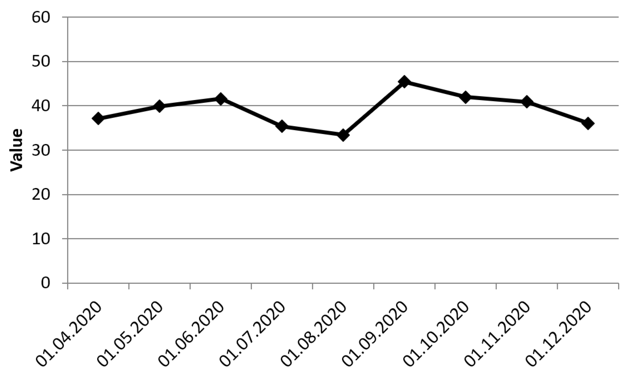
The time series of the indicator “Percentage of equipment operation time” will be analyzed. This indicator reflects the efficiency of the use of equipment. The machining center may, at other times, be in a state of downtime, scheduled maintenance, changeover, or emergency repair. An indicator of effective planning of equipment operation modes will be the maximization of the percentage of equipment operation time according to the production program. The states of downtime, changeovers, planned repairs of the time spent and frequency of occurrence should be minimized. Furthermore, the state of emergency repair must be eliminated.

For example, consider the time series of the machining center. This time series characterizes the indicator “Percentage of equipment operating time”. In the time interval from May to December, the values contain the average monthly estimate. The time series is shown in Figure 3. The numerical data of the time series in

Table 1. Time series of equipment operating time percentage.

Monthly Time Point	Working Hours According to the Program, %
30 April 2020	37.13
31 May 2020	39.89
30 June 2020	41.6
30 July 2020	35.39
30 August 2020	33.46
30 September 2020	45.42
30 October 2020	41.99
30 November 2020	40.93
30 December 2020	36.07

are given.

The time series model by using the algorithm described in Section 4 is formed. Previously, the time series could be smoothed by using existing methods to improve their tendencies. The time series presented in the experiment will not be smoothed since it is short and already contains aggregated values. Furthermore, smoothing will result in the loss of information.

The first step of the time series modeling is the computing of numerical tendencies. The result is shown in

Table 2. Time series tendencies.

Monthly Time Point	Value of the Tendency
31 May 2020	2.76
30 June 2020	1.71
30 July 2020	−6.21
30 August 2020	−1.93
30 September 2020	11.96
30 October 2020	−3.43
30 November 2020	−1.06
30 December 2020	−4.86

.

The universe of fuzzy sets must cover a numeric interval in the range $[-6.21,12.96]$; in other words, the boundaries as the minimum and maximum value of the obtained time series tendencies are defined.

As an example, let us choose three type-2 fuzzy sets for the fuzzification of a numerical interval. Such a rough partition will help to demonstrate the efficiency of correcting type-2 fuzzy set intervals boundaries. This results in a set with an indication of intervals for the lower and upper membership functions:

$$\tilde{A}=\{{\tilde{A}}_1(-6.21,0.15)(-7.21,1.15),{\tilde{A}}_2(0.15,6.2)(-0.85,7.2),{\tilde{A}}_3(5.2,11.96)(4.2,12.96)\}.$$

A set of fuzzy labels are created and extracted from the context by an expert method:

$$\{{\tilde{A}}_2^C,A_2^C,A_2^C,{\tilde{A}}_1^C,{\tilde{A}}_1^C,{\tilde{A}}_3^C,{\tilde{A}}_1^C\},{\tilde{A}}_i^C\in U.$$

where for type-2 fuzzy sets, ${\tilde{A}}_i^C$, the following parameters are defined:

$${\tilde{A}}^C=\{{\tilde{A}}_1^C(-6.21,0)(-6,1),{\tilde{A}}_2(0.05,6.2)(-1,8),{\tilde{A}}_3(5.2,11.96)(7,12)\}.$$

Fuzzification of the original numerical time series is performed:

$$\{{\tilde{A}}_2,{\tilde{A}}_2,{\tilde{A}}_1,{\tilde{A}}_1,{\tilde{A}}_3,{\tilde{A}}_1,{\tilde{A}}_1,{\tilde{A}}_1\},{\tilde{A}}_i\in U$$

The fuzzy rules of the extracted time-series tendencies are represented as follows:

$$Rules=\{{\tilde{A}}_2\to {\tilde{A}}_2,{\tilde{A}}_2\to {\tilde{A}}_1,{\tilde{A}}_1\to {\tilde{A}}_1,{\tilde{A}}_1\to {\tilde{A}}_3,{\tilde{A}}_3\to {\tilde{A}}_1,{\tilde{A}}_1\to {\tilde{A}}_1,{\tilde{A}}_1\to {\tilde{A}}_1\}$$

The fuzzy rules of the tendencies taken out of context are presented as follows:

$$Rule{s}^C=\{{\tilde{A}}_2^C\to {\tilde{A}}_2^C,{\tilde{A}}_2^C\to {\tilde{A}}_1^C,{\tilde{A}}_1^C\to {\tilde{A}}_1^C,{\tilde{A}}_1^C\to {\tilde{A}}_3^C,{\tilde{A}}_3^C\to {\tilde{A}}_1^C\}$$

The rule sets are merged:

$$\begin{array}{c}\hfill Rule{s}^C\cup Rules=\{{\tilde{A}}_2\to {\tilde{A}}_2,{\tilde{A}}_2\to {\tilde{A}}_1,{\tilde{A}}_1\to {\tilde{A}}_1,{\tilde{A}}_1\to {\tilde{A}}_3,{\tilde{A}}_3\to {\tilde{A}}_1,\\ \hfill {\tilde{A}}_1\to {\tilde{A}}_1,{\tilde{A}}_1\to {\tilde{A}}_1,{\tilde{A}}_2^C\to {\tilde{A}}_2^C,{\tilde{A}}_2^C\to {\tilde{A}}_1^C,{\tilde{A}}_1^C\to {\tilde{A}}_1^C,{\tilde{A}}_1^C\to {\tilde{A}}_3^C,{\tilde{A}}_3^C\to {\tilde{A}}_1^C\}\end{array}$$

Then, correction of type-2 fuzzy sets based on the intervals set boundaries $A_i^C$ is performed. Figure 4 shows a time series based on this rule set.

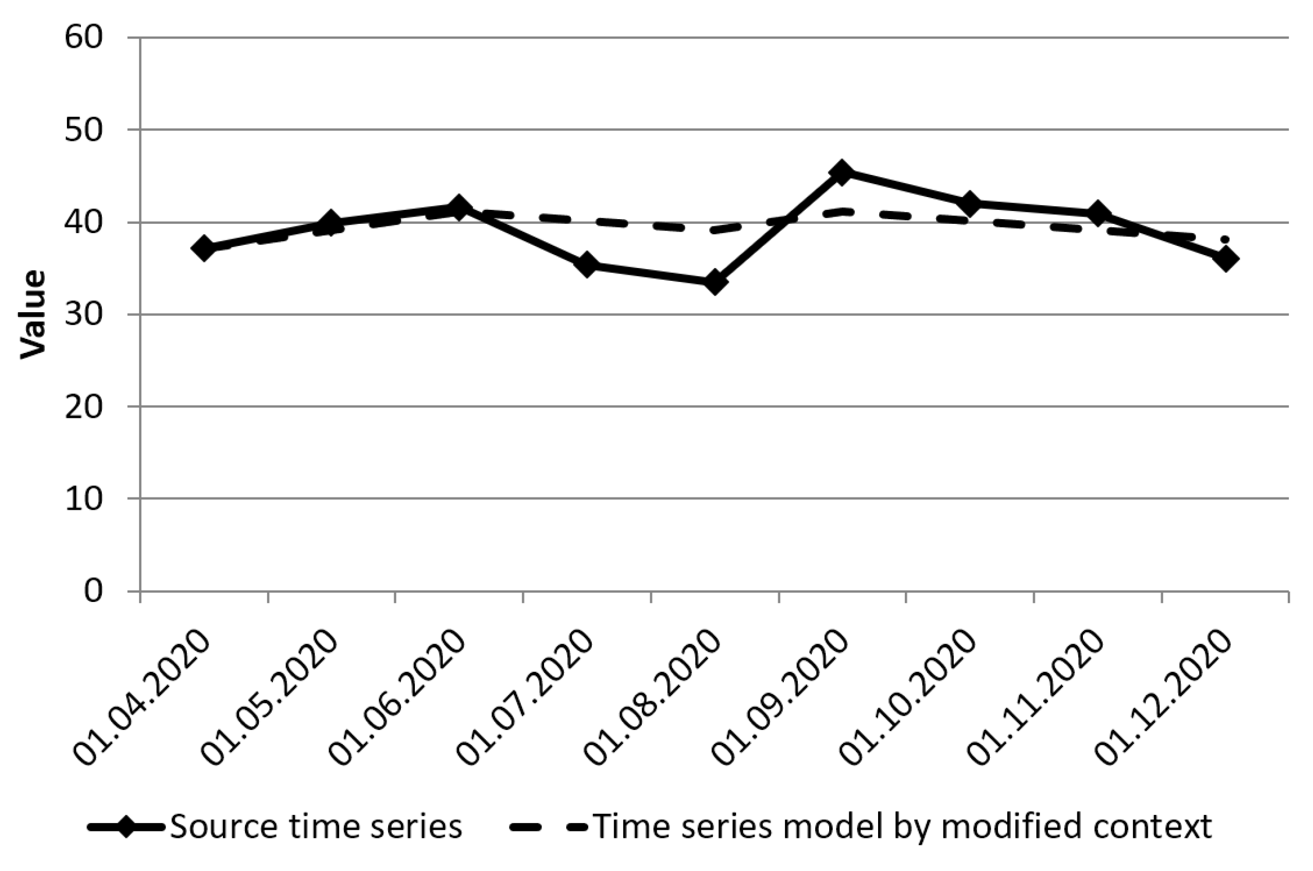
Now, consider the case of a context change. The rule base of the sets $A_i^C$ and the boundaries of the type-2 fuzzy set intervals will change. This case will be considered when the requirements for the equipment operability increase in production. Analysis of the textual information of such a case makes it possible to distinguish an “increase” tendency for the “equipment operability” indicator. This information will serve as a summary of the modified context. The rule base will be presented as follows:

$${\tilde{A}}_2^C\to {\tilde{A}}_2^C,{\tilde{A}}_2^C\to {\tilde{A}}_1^C,{\tilde{A}}_1^C\to {\tilde{A}}_1^C,{\tilde{A}}_1^C\to {\tilde{A}}_2^C,{\tilde{A}}_2^C\to {\tilde{A}}_1^C$$

For type-2 fuzzy sets ${\tilde{A}}_i^C$, the following parameters are defined:

$${\tilde{A}}^C=\{{\tilde{A}}_1^C(-6.21,0)(-3,1),{\tilde{A}}_2(0.05,6.2)(-1,5),{\tilde{A}}_3(5.2,11.96)(5,10)\}.$$

Figure 5 shows a time series based on the changed context.

We can then conclude that the context information can influence the construction of the time series model. The benefits of this approach would be:

• The ability to adjust the time series model using external information from the context;
• The ability to build a time series model when the number of $A_i$ components is limited (not enough time series points);
• The ability to search for anomalies in the received time series to generate recommendations.

The difference from other modeling methods, such as methods of exponential smoothing, methods of fuzzy modeling, and compression of the time series [11], is the possibility of including external information from the context of the problem domain of the time series into the model. Analysis of texts can provide such information about the modeled object. Indicators in linguistic form can be expressed. Information from external knowledge bases can also be retrieved.

8. An Experiment on Contextual Time Series Forecasting

According to the Figure 2, the experiment involves working with context and time series models.

For example, we use the following fragment of the ontology that represents the context:

$$\begin{array}{cc}\hfill & bound:Intervalaccept:IntervalotDesc:DescotDef:Def\hfill \\ \hfill & otTS:TSoperationalTime:O^{num}department:O^m\hfill \\ \hfill & \left(otTS,otDesc\right):hasDesc\left(operationalTime,otTS\right):hasTS\hfill \\ \hfill & \left(operationalTime,otDef\right):hasDef\left(department,operationalTime\right):hasProperty\hfill \end{array}$$

The ontology describes the same object and its properties, as in the previous section. The main management object is department, the analyzed object property is operationalTime. In ontology, the time series represents property values otTS.

The enterprise equipment gives a lot of monitoring indicators. We analyze the operational time of each machine. The time series is one of the output datasets of block 1.

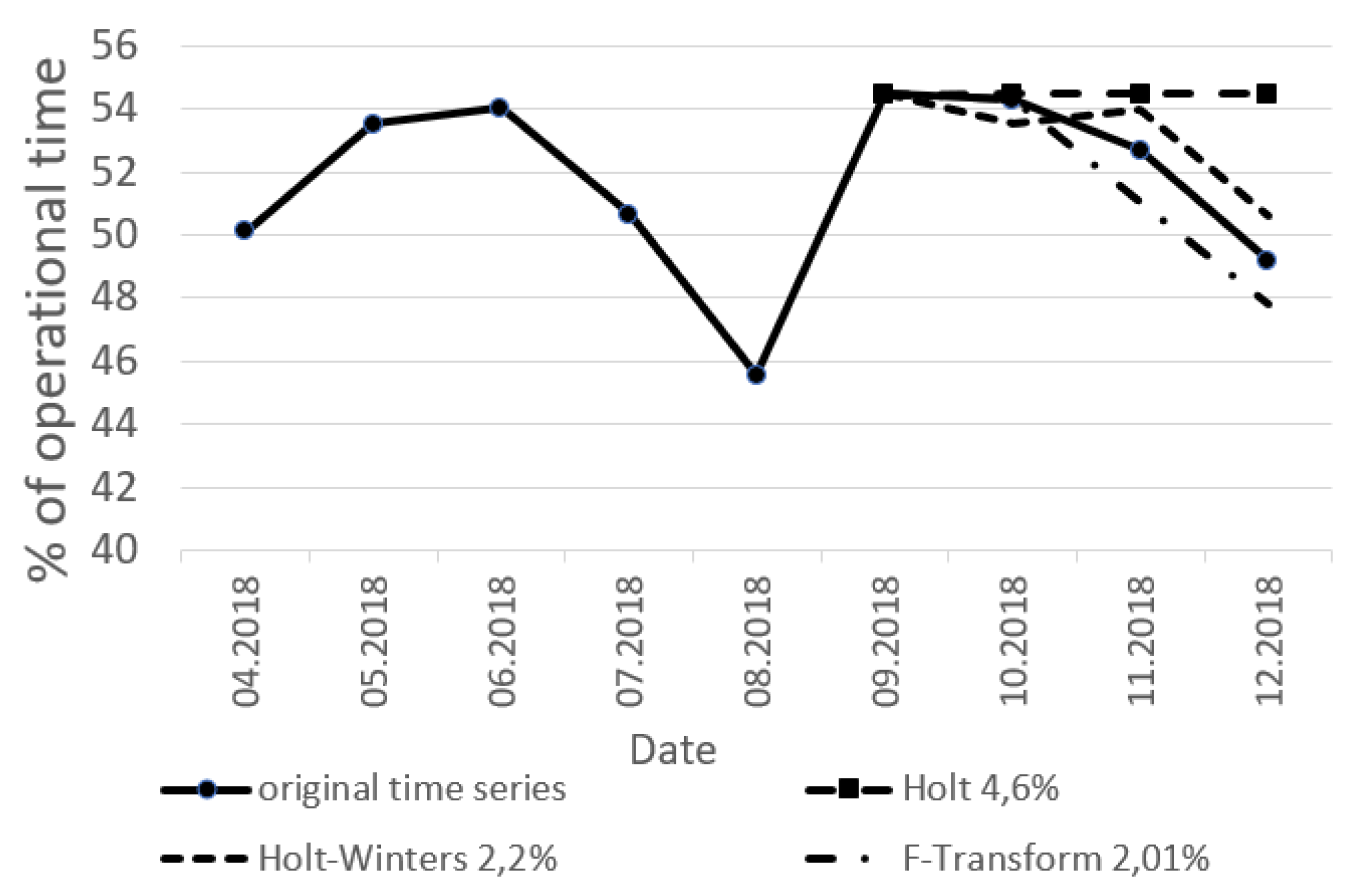
Time series model construction is according to block 3.1 of the scheme. For example, the following time series forecasting methods are used: exponential Holt time series model, exponential Holt–Winters time series model with seasonal component. For comparison, we use F-Transform [29] with the “If–Then” rule base.

The part of ontology that describes the exponential Holt time series model:

$$\begin{array}{cc}\hfill & timeSeriesLength:Intervalholt:M\hfill \\ \hfill & \left(timeSeriesLength,5\right):hasMinValue\left(timeSeriesLength,MAX\right):hasMaxValue\hfill \\ \hfill & \left(holt,true\right):hasTendency\left(holt,false\right):hasPeriod\left(holt,false\right):hasSeason\hfill \\ \hfill & \left(holt,true\right):hasSmooth\left(holt,false\right):hasFuzzy\left(holt,timeSeriesLength\right):length\hfill \end{array}$$

The length of the forecast is 3 points, because of the small length of the time series.

Without using the context, we can build a forecast on a test interval, see Figure 6, a Forecast estimation by the SMAPE criterion [36] is made.

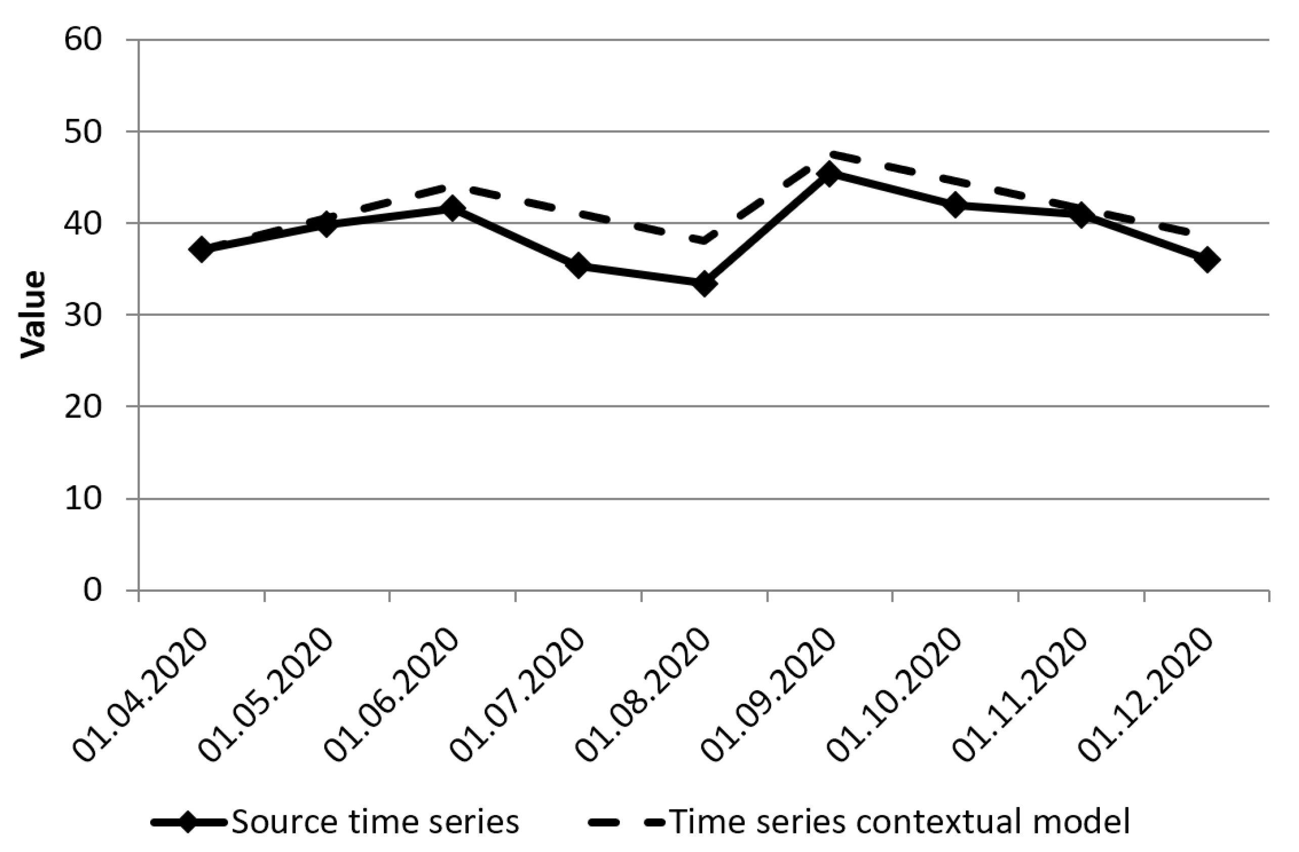
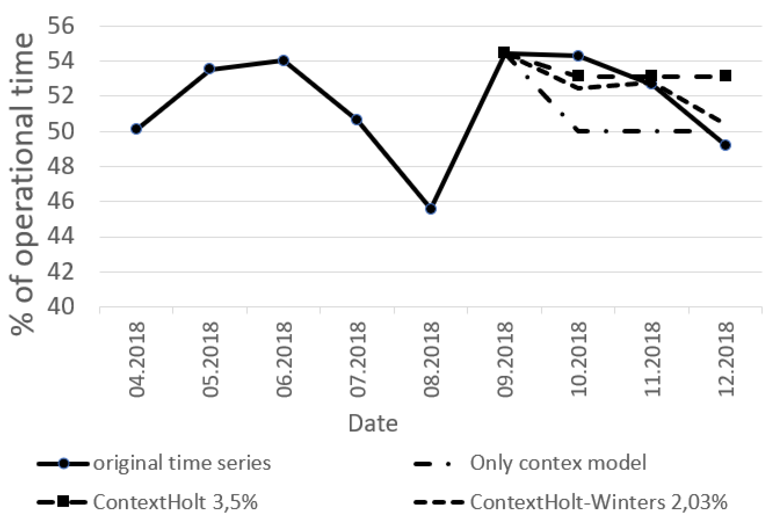
As the next step, according to the expression (13), we can build forecasts for the time series, see Figure 7.

According to block 4, forecasts can use context information for the time series model (10):

$$\begin{array}{cc}\hfill & \left(bound,0\right):hasMinValue\left(bound,100\right):hasMaxValue\left(accept,50\right):hasMinValue\hfill \\ \hfill & \left(accept,60\right):hasMaxValue\left(otDesc,50\right):hasBase\left(otDesc,0\right):hasTendBase\hfill \\ \hfill & \left(otDesc,5\right):hasTendDelta\left(otDesc,bound\right):hasBound\left(otDesc,accept\right):hasAccept\hfill \\ \hfill & \left(otDef,50\right):hasBase\left(otDef,0\right):hasTendBase\hfill \end{array}$$

The model parameter $w_{Def}$ is set equality to 0.3. The weight of the numerical model forecast in contrast with the context forecast is greater.

The formed context model components allow the following actions:

• Check and filter the model restrictions on seasonality, frequency. Holt, Holt–Winters, F-Transform time series models satisfy this requirement.
• The following forecasting models satisfy the expression (14): Holt, Holt–Winters. The F-transform method with the obtained value of the last point at 47.81 is not suitable by the requirement: the forecast values are within acceptable boundaries (50, 60).

We can conclude that the forecast of the operational time of the equipment in the department will decrease. The forecasted levels of the time series match with the contextual restrictions.

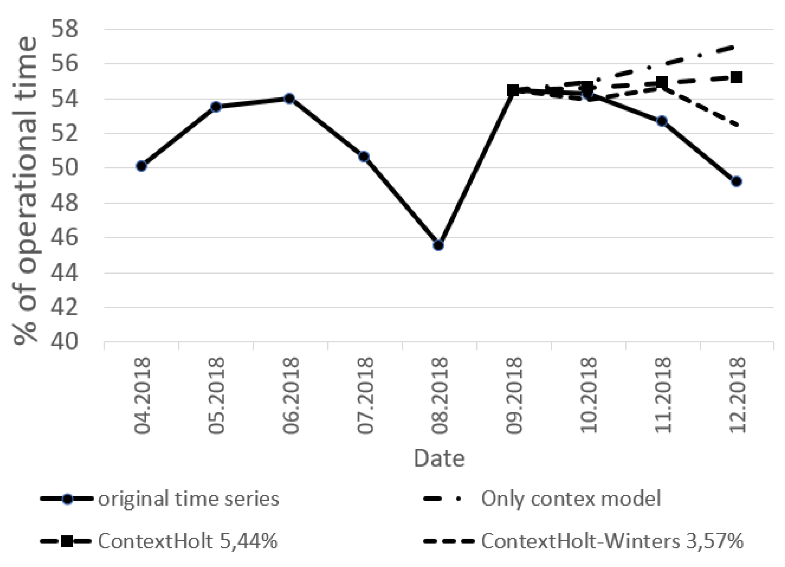
The model components can take the following form in case of context changes (e.g., production volume increases):

$$\begin{array}{cc}\hfill & \left(bound,0\right):hasMinValue\left(bound,100\right):hasMaxValue\left(accept,50\right):hasMinValue\hfill \\ \hfill & \left(accept,60\right):hasMaxValue\left(otDesc,50\right):hasBase\left(otDesc,1\right):hasTendBase\hfill \\ \hfill & \left(otDesc,5\right):hasTendDelta\left(otDesc,bound\right):hasBound\left(otDesc,accept\right):hasAccept\hfill \\ \hfill & \left(otDef,50\right):hasBase\left(otDef,1\right):hasTendBase\hfill \end{array}$$

The forecast for these conditions show on the Figure 8.

This forecast is given as an example demonstrating the change in forecast results due to the context change.

The Holt–Winters time series model does not satisfy restrictions (Equation (14)), although it shows the best estimate for SMAPE. It needs to select another model for time series forecasting.

The experiment shows that the context information in time series modeling allows increasing the forecasting quality due to choosing a better model or a model that matches the decision-maker expectations.

9. Discussion

The described results show that the time series model can widely use the concept of an information granule. Time series granulation can be based on model components, such as tendencies and others. However, an information granule can reflect many other attributes of objects in the problem area: expert opinions, knowledge and correlation with other object parameters. The opportunity lies in the hybridization of the time series analysis methods, considering the context of the problem area.

Another main advantage of the proposed approach is the explanatory component. Recommender systems based on the proposed principle can, at any time, provide confirmation of the issued conclusion. This is possible due to the connection between the analyzed time series and the objects of the real world. For example, during the analysis of the text materials of the context, it will be obvious which parameter of which object will be analyzed. The fuzzy models help develop easy-to-use numerical representations of indicators, or the most general, fuzzy ones.

The proposed approach at every stage of analytics of the dynamic data can be embedded: descriptive analytics, predictive analytics, and prescriptive analytics. The advantage is that we can analyze a separate indicator and form conclusions about the forecast, and vice versa, the use of predicting and prescription for the behavior of some objects helps to describe others.

The disadvantages of the proposed approach include high computational complexity, the use of an expert to form the ontology of the problem area, or the use of methods for extracting and studying object knowledge.

Therefore, the goal of further research will be an extended analysis of the dynamic data of related objects in context. The task of advanced fuzzy model studies is to consider the restrictions on the choice of intervals of type-2 fuzzy sets when approximating time series.