A Comprehensive Fuzzy Decision-Making Method for Minimizing Completion Time in Manufacturing Process in Supply Chains

Abstract

In manufacturing firms, there are many factors that can affect product completion time in production lines. However, in a real production environment, such factors are uncertain and increase the adverse effects on product completion time. This research focuses on the role of internal factors in small- and medium-scale supply chains in developing countries, enhancing product completion time during the manufacturing process in fuzzy conditions. In the first step of this research, a list of factors was found clustered into six main groups: technology, human resources, machinery, material, facility design, and social factors. In the next step, fuzzy weights of each group factor were determined by a fuzzy inference system to reflect the uncertainty of the factors in utilizing product completion time. Then, a hybrid fuzzy–TOPSIS-based heuristic is proposed to generate and select the best production alternative. The outcomes showed that the proposed method could generate and select the alternative with a 10.13% lower product completion time. The findings also indicated that using the proposed fuzzy method will cause less minimum variance compared to the crisp mode.

1. Introduction

The manufacturing sector plays a crucial role in utilizing the economy of a country. According to the statistics that are reported by the “Statista” website, more than 37.4% of the gross domestic product (GDP) of Malaysia belongs to industries (Figure 1).

1.1. A Common Major Shortcoming in Many Manufacturing Firms

Many industries do not pay enough attention to the factors that can enhance (or decline) productivity. Such ignorance yields many problems, for example sometimes failing to manufacture enough products to fulfill the market demand. Such problems often can be found in small- and medium-scale companies in developing countries. Figure 2 represents the number of bankrupted companies in Malaysia in 2019.

Such phenomena can lead to bankruptcy or at least slow the growth of a company. Successful firms, by contrast, have handy strategies to improve and develop their businesses. Besides, failing to pay enough attention to success factors in production can cause immediate bankruptcy for many young businesses. Figure 3 indicates the number of registered companies in Malaysia from 2008 to 2018.

Although this number shows the total number of companies in all sectors (including manufacturing and services), at the same time, even if 50% of this value belongs to manufacturing industries, it is still significant.

• Uncertain conditions that surround the manufacturing firms

One important thing that must be considered about manufacturing firms is that the factors that can influence the production rate of manufacturing companies may be different from one company to another due to their surrounding environment.

Therefore, this research tries to find the significant factors in minimizing the processing time of manufacturing firms in Malaysia and, then, propose a new method to choose the best manufacturing strategy, according to the actual production environment of a company.

• Can uncertainty increase the risk of bankruptcy in manufacturing companies, and how can it be prevented by using the fuzzy method?

Some preconceptions show positive correlations between increasing uncertainty and the chance of bankruptcy in a manufacturing firm. However, this idea will be explored in Section 2. Uncertainty can increase entropy in manufacturing companies. This research aims to find which uncertainty factors will play critical roles in a completion time of a product (as the primary goal of this research) in a company and, then, how to prevent such uncertainty in manufacturing companies using the fuzzy method.

1.2. Managerial Implications of the Research

In today’s world, the fundamental or essential part of the developing countries’ economy mainly relies on their industries. The more advanced industries mean more products in terms of quantity and quality, resulting in less importing and more exporting of goods. Therefore, it is crucial to propose methods to skyrocket the production factors such as time. During the last half-century, many research studies have been carried out to utilize production line performance.

The outcomes of this research provide a framework that will help managers in various industry sectors to conduct an accurate study in their production lines, identify the status of effective factors in increasing (or decreasing) product completion time, and select a better production strategy for manufacturing more products with higher quality.

The rest of the paper includes a detailed literature review to find the critical factors. Then, a fuzzy inference system will be proposed to determine the fuzzy weights of the group factors. Afterward, a fuzzy–TOPSIS heuristic will be proposed to generate different alternatives and, then, select the best one in terms of the total product completion time. To evaluate the performance of the proposed method, using DOE, several experiments will be designed. Then, the outputs will be examined by using indicators. The results of the proposed method will be compared to the crisp mode to show the effect of uncertainty on product completion time.

2. Decision-Making Methods in Minimizing Product Completion Time

Various decision-making methods have been widely used for various problems in industries. Decision-making methods are those methods used to select one (or more parallel) feasible solutions among thousands, millions, or even billions of possible solutions. Choosing the appropriate decision-making method can help to make a correct decision in a reasonable time. Each paper is cited in the appropriate content and sub-content where relevant. This section will explain several important decision-making methods for minimizing the production and cycle time in manufacturing systems.

2.1. Technology

Perhaps using appropriate technology can be considered the most influential reason for determining product completion time. Using old technologies is time consuming and can waste many energies.

In modern technologies, automation facilitates the production cycle by replacing many hand jobs with robots. Moreover, using modern technologies eases the tasks and increases production speed. In this section, some research studies that focused on minimizing completion time will be reviewed.

Xu et al. compared two types of ACO (job sequence and batch sequence) for minimizing the total completion time in a single batch processing machine [1]. Irdem et al. mentioned that the mean cycle time increases nonlinearly with resource utilization [2]. They proposed a computational case study to evaluate the convergence behavior between linear programming (LP) methods and simulations as two commonly used methods for scheduling the manufacturing systems.

Ramezanian et al. proposed a GA and Tabu search (TS) for solving a MILP aggregate production planning (APP) model to determine the production amount, inventory level, and the required workers [3]. Shah and Ierapetritou discussed that by increasing the number of production sites in supply chains, the tractability of the whole system becomes more challenging in a supply chain network. Therefore, they proposed an integrated planning and scheduling problem for the multi-site/multi-product batch plants. They considered the augmented Lagrangian decomposition method to solve their model [4]. Ning et al. tried to maximize the belief degree of obtaining the profit compared to the forecasted profit. For this purpose, they developed a multi-product aggregate production-planning model under uncertain conditions where market demand, production cost, and subcontracting cost are stochastic [5].

S.-C. Wang and Yeh used an IP programming method for formulating the APP model. As a practical test, they used data from a gardening equipment manufacturer, solving their model using particle swarm method (PSO), and compared their result with GA [6]. Díaz-Madroñero et al. provided an invaluable review of the literature on tactical production planning. Their findings showed that modeling approaches such as LP, IP, and MILP were the most frequently used in tactical production planning methods. One shortcoming they mentioned is that most of the research studies contained numerical experiments with randomly created instances [7]. In contrast, less validated their methods/approaches by applying them in practice. Gansterer et al. tried to find the worthy settings for lead time, safety stock, and lot size in production planning by developing a framework for hierarchical production planning in a make-to-order environment. As a part of the framework, they developed a mathematical model and used variable neighborhood search to find the best result [8]. Kodialam et al. proposed a new method for minimizing the completion time by considering a lower bound for each task [9]. Rossi et al. proposed a hybrid MRP procedure and an LP method to overcome lead times. Their outcomes indicated that regardless of requiring lead times, the new method could provide feasible plans of orders [10]. L. Yang et al. addressed a supervised fuzzy inference system for minimizing job completion time estimation, which worked based on estimating the completion times for different tasks under different conditions [11]. Żywicki et al. mentioned that in some cases, different delivery times that customers request could cause barriers for manufacturing systems, as it can influence their scheduling process. Therefore, they proposed software to provide a portfolio of highly individualized product times by anticipating standard times for them [12].

J. Wang et al. focused on cycle time forecasting (CTF) in semiconductor wafer fabrication systems [13]. For this purpose, they addressed a supervised parallel computing method for data-intensive cycle time prediction for large datasets. They showed that the proposed method could compute faster and outperform the other CTF methods in terms of mean absolute and standard deviation (Std. Deviation). Rauch et al. illustrated that it is difficult to synchronize between fabrication and on-site installation [14]. Therefore, they proposed an axiomatic design-based method for real-time-capable production planning and control to minimize time dependency in the value chain. Rubaiee and Yildirim proposed a new multi-objective method for scheduling manufacturing systems to minimize the total completion time and energy cost [15]. Under time-of-use electricity tariffs, which is a mixed-integer mathematical programming model, they, then, used hybrid holistic ant colony optimization algorithms (ACO) for solving their problem. Huang et al. developed a mathematical model to simulate real-time dynamics of the system in a multi-product serial production line [16]. Then, they addressed a hybrid machine learning techniques and analytical system model to predicting product completion time, which worked based on considering the lower bound of product completion time that represented the least possible product completion time when assuming no random downtime in the system. Then, they applied a deep-learning model to forecast the variance among the lower bound and actual product completion time. de Curs et al. addressed an extended fuzzy-AHP (EF-AHP) for the risk assessment process for supply chains. They showed that the proposed EF-AHP could provide better results than fuzzy-AHP in terms of obtained priority weights against the normalized scores of criticality [17].

Fischer et al. argued that anticipating completion time in manufacturing systems must combine actual completion times and self-adjusting prediction completion times [18]. Choy et al. argued that emerging job tardiness in the production schedule would dramatically influence the harmony of different jobs on the shops in a manufacturing system. Therefore, they developed a hybrid scheduling decision support model, where the aim was minimizing job tardiness. They solved the model with GA. Kopanos et al. focused on the packing stage in a dairy production firm. They stated timing and capacity constraints as the essential factors in generating feasible production plans. To overcome such shortcomings, they proposed a MILP programming model, where quantitative and qualitative objectives have been considered. Erol et al. presented a new multi-agent-based real-time scheduling method for automated guided vehicles (AGVs) in dynamic conditions when planning operations dynamically [19]. Multi-agent-based systems, a newly maturing area of distributed artificial intelligence, provide effective mechanisms for managing such dynamic operations in manufacturing environments. Later, Gen and Lin proposed a multi-objective evolutionary algorithm to solve job shop scheduling problems, AGV in flexible manufacturing systems, and integrated process planning and scheduling [20].

Kapanoglu et al. proposed a pattern-based GA for scheduling intelligent manufacturing systems. Their research aimed to find the optimum sequence of the disks for each robot, where the objective was reducing the coverage completion time [21]. K. Li et al. addressed a supervised method for minimizing total completion time in uniform machine scheduling problems, where the agent “technology” is introduced to realize the role of the automation process in scheduling using the intelligence of the machines [22]. Angius et al. proposed a method to analyze the cumulated output and the lot completion time moments in unreliable manufacturing systems characterized by general Markovian structures. Their outcomes showed that the proposed method could help analyze the dependency of the output variability and the service level of a system [23]. Mokhtari and Salmasnia addressed a neighborhood search algorithm for reducing the processing time of a multiple-machine manufacturing system. Then, they used an evolutionary clustering search, where iterative clustering is applied to identify the subspace [24].

Z. Li et al. focused on the energy consumption and cycle time in two-sided assembly lines. For this purpose, they developed a new mixed-integer programming (MIP) model, where a robotics-based assembly line is taken into consideration [25]. To solve their model, they used simulated annealing (SA). Costa et al. used the MIP model for a parallel scheduling machine with periodic tool changes to minimize total completion time. Then, a hybrid genetic algorithm (GA) was developed, and the outcomes were compared with three alternative methods arising from the literature [26]. Smutnicki focused on a cyclic production system, where a fixed mixture of various goods is produced in a short series. In order to solve their model, a method is proposed to find the minimal cycle time for a fixed-job processing order [27]. X.-J. Chen et al. investigated the problem of supporting structure in layer-based additive manufacturing (AM). They argued that it could cause increasing fabrication time, while decreasing surface quality. To overcome such shortcomings, they proposed an optimizer that could reduce supporting structures by identifying the prime printing direction [28]. The reviewed research studies in this section showed that various decision-making methods have been used successfully to minimize the completion time.

2.2. Human Resources

One crucial factor that can influence product completion time is human resources. In this section, research studies related to the role of human resources in manufacturing systems will be divided into three main categories: human resources scheduling, lack of sufficient human resources, and human resources skills.

A Delgoshaei and A Ali reviewed different human resources scheduling methods in cellular manufacturing systems (CMS) [29]. Aryanezhad et al. developed a multi-period scheduling model for worker assignment [30]. Süer et al. dealt with minimizing job tardiness in CMS by human resources scheduling and cell loading. For this purpose, they used mathematical models. They reported that total tardiness is reduced in their models, while the crew size increases [31]. Delgoshaei and Ali proposed a hybrid ant colony optimization (ACO) and Tabu search (TA) to scheduling temporary and skilled workers in dynamic CMS, where promoting workers using training was taken into account [32].

Human resources skills can be considered a critical factor in increasing the speed of performing tasks in manufacturing systems. Therefore, many research studies focused on the role of promoting human resources in minimizing manufacturing cycle time. Aryanezhad et al. developed a multi-period scheduling model for worker assignment, where three levels for worker skills were considered [30]. Satoglu and Suresh focused on cross-training during workers’ assignments [33]. Delgoshaei et al. proposed a new method for scheduling temporary and fixed workers in a manufacturing company, which helps to improve the production cycle time. Their model considered different workers’ skill levels and assigned tasks to them, according to their skill level [34]. Therefore, human resources can be considered an important factor that can influence product completion time.

2.3. Social Atmosphere in Manufacturing Systems

Providing a friendly production environment supported by solid teamwork relations can increase the performance of a manufacturing process. Workers in a calm and friendly environment seem more active than in a place with much stress and tension. Ounnar and Pujo mentioned that for a company to be safe in competition, it is vital to look for new methods for controlling their workshop [35].

To continue, some critical research studies in HR scope with the impact of production environment on product completion time will be investigated.

Generating high-performance teamwork can be considered an essential factor in manufacturing engineering to boost system performance. Fitzpatrick and Askin focused on the correlations between humans and technology to create good effective teamwork forming. In their research, they tried to enhance the HR performance by generating teams in manufacturing cells. Cesaní and Steudel tried to assign workers jobs, where work sharing and balancing were considered [36]. Ounnar and Pujo proposed a new approach for controlling the workshop using the Holonic paradigm in a decision-making multi-criteria analysis [35].

Decisions that are taken by top management can skyrocket or drop production speed. An appropriate decision in the correct time and place will boost production speed drastically. For example, hiring new workers, promoting current workers, buying a new machine, and purchasing raw materials with better quality are among the top management decisions that can increase system performance. Q. Li et al. proposed a multi-objective method for minimizing average salary and maximizing average satisfaction simultaneously. Their model aims to figure out the best worker assigning the cross-trained laborers [37]. Liu et al. focused on the scheduling cloud manufacturing system, where multiple users are allowed to request various services from management simultaneously. They proposed a cloud manufacturing multi-task scheduling model, which integrated task workload modeling with several other essential ingredients regarding services and could help investigate the effects of different workload-based task scheduling methods on total completion time and service utilization [38]. As a conclusion, teamwork is considered among the important factors that was investigated in utilizing the manufacturing system’s performance.

2.4. Composition of Material

The role of raw material composition in the production process is undeniable. In the literature review, many studies investigated the effects of raw material on producing a particular product. Due to the enormous number of industries, it is impossible to investigate raw materials’ role in all different industries. Therefore, in this section, some case studies will be presented. For example, Castellano et al. showed the role of raw materials composition on the quality of pellets obtained from different woody and nonwoody biomasses [39]. Afolabi et al. focused on the role of raw materials in the glass-making industry’s productivity [40]. Z. Chen et al. investigated the effects of raw materials on the silicon furnace process [41]. However, one question to be answered in this research is whether choosing different raw materials can influence product completion time? Answering the above question can light up the importance of material in minimizing product completion time in manufacturing systems.

2.5. Broken Machinery and Maintenance

One primary reason for increasing processing time is emergency machine failure during production time that can waste much time. Therefore, during the last three decades, several invaluable research studies have been carried out to minimize machines’ downtime. Singh et al. proposed a method for ranking the barriers in performing effective maintenance strategies in manufacturing systems [42]. According to their findings, lack of top management support, an effective measuring indicator such as overall equipment effectiveness (OEE), and lack of strategic planning and implementation are the most important reasons for an ineffective maintenance process in manufacturing systems. Delgoshaei and Naserbakht proposed a new method for minimizing plane downtime in airport maintenance shops using a metaheuristic method [43]. Seiti and Hafezalkotob illustrated the role of maintenance in enhancing the performance of a manufacturing system in terms of availability, product quality, and low costs [44]. They argued that insufficient information about equipment failure likelihood causes quantitative models not to be effective in manufacturing environments. They proposed a fuzzy model, where a fuzzy set expresses the reliability of an equipment. Then, using the outcomes of the method, a risk-based TOPSIS was developed to schedule preventive maintenance. The aforementioned results show that an appropriate maintenance plan can affect product completion time positively. Hence, maintenance can also be considered an effective factor in minimizing product completion time.

2.6. Facility Layout

The way that machines are located in different stations of a company directly impacts production cycle time. Aidin Delgoshaei and A. Ali reviewed different types of grouping machines in manufacturing shops using clustering techniques [45].

Material transferring between different machines inside a company can take time. In manufacturing studies, two types of primary material transferring can be recognized: internal material transferring and outer material transferring. While external material transferring refers to delivering raw material to the company or transporting final product to retailers or customers, internal material transferring refers to transporting in-process material between machines and between shops. Although delays in external transporting such as delays in receiving raw material or delivering the final product can be considered a delay and cause customer dissatisfaction, they cannot cause increases in product manufacturing cycle time. Thus, internal transferring between machines and shops/cells will be a reason for increasing product manufacturing cycle time. Delgoshaei and Gomes proposed a supervised method for dispatching materials in process inside a manufacturing shop to prevent delays in the processing tasks of machines [46].

Delgoshaei et al. explained all possible material transferring methods in CMS and reviewed the literature on material transferring in manufacturing systems [47]. Haleh et al. addressed a new method for minimizing in-shop material movements using a hybrid revised TOPSIS and Memetic algorithm. Their method was also capable of minimizing the cell load variation [48]. Reviewing the opted references in this section reveals that facility layout should be considered an effective factor, while choosing the best alternative for minimizing product completion time.

2.7. Uncertainty and Fuzzy Logic

In an actual manufacturing plant, various factors must be considered to make a schedule. Graves dealt with the role of uncertainty in the production planning process. They argued that current planning systems do not provide adequate decision support for tactical decisions [49]. Zhong et al. argued that many components cause uncertainty and complexity in the production environment [50].

Some factors include human resources, proceeding time of a task, setup time, loading and unloading times, quality of materials, and worker’s speed. However, most such factors are not fixed and can be different from time to time, according to different conditions surrounding the manufacturing plants. In the past, most manufacturing systems’ research studies considered fixed factors; however, during the last two decades, scientists became aware of the importance of uncertainty and found that uncertain factors can reject or change a possible solution.

Macal and North used agent-based simulation to study the individual behaviors in healthcare supply chains and the stock market, where the aim was to predict the success of marketing campaigns to outline the system’s future needs [51]. Albey et al. declared the value of demand forecast information in production planning. In their research, forecast evolution and inventory theory ideas were integrated to plan work releases into a production facility, while product demands were not specific and differed from period to period. The Martingale model of forecast evolution is used to model demand through the time horizon [52]. Fuzzy methods are successfully used in metaheuristic algorithms to consider the uncertainty. A fuzzy-genetic algorithm is proposed for a container dispatching cost estimation model to overcome the container supplements problem [53]. A fuzzy-genetic algorithm is developed in another industrial sector to address the customer attributes and design parameters in an intelligent product design problem [54].

2.8. TOPSIS

TOPSIS is a decision-making method to select the best alternative among available alternatives by considering different weights that have been widely used for managerial and engineering problems. It is classified as a multi-attribute decision-making method (MADMs).

Tyagi et al. developed a two-step approach, which worked based on analytic hierarchy process (AHP) to select the best alternative and TOPSIS for order preference by similarity to ideal solution in electronic supply chain management (e-SCM) [55]. They applied their approach to an Indian automobile industry, where eight criteria and five alternatives were considered. Nilsson et al. discussed that many existing multi-criteria decision analysis methods (MCDA) used in forest management planning could compare and evaluate a short number of management plans. Such phenomena increase the risk in the decision process. Therefore, they proposed a hybrid AHP and TOPSIS to improve the performance of evaluating many strategic forest management plans [56]. Felfel et al. developed a multi-product transportation scheduling method for the SCM problem, where the aims were maximizing the profit and product quality level simultaneously. Their solving method consisted of three steps using the epsilon-constraint method to generate Pareto optimal solutions, ranking the alternatives with TOPSIS and, then, using VIKOR to evaluate the outcomes of the TOPSIS [57].

Kaya and Kahraman focused on sustainability criteria (economic, social, and environmental factors) in scheduling manufacturing systems. They argued that selecting an effective energy technology requires keen eyes on conflicting quantitative and qualitative evaluation criteria. For this purpose, a modified fuzzy–TOPSIS is used to select the best energy technology alternative, where fuzzy pairwise comparison matrices determine the weights of factors [58]. Bas proposed a hybrid SWOT–fuzzy–TOPSIS and AHP for an electricity supply chain, where a quantitative strengths, weaknesses, opportunities, and threats (SWOT) framework was used to formulate a strategic plan based on the elements proposed qualitative framework [59]. Sahu et al. developed a multiple-criterion appraisal index supply chain for selecting suppliers among existing alternatives. For this purpose, they proposed a new interval-valued fuzzy number set combined with the modified TOPSIS. Their method used a fuzzy mathematical equation to compute first-level measures’ priority weights and appropriateness ratings [60].

Kia et al. used fuzzy-based TOPSIS to rank various alternative productions in the faucet industry under uncertain conditions, where five criteria of profitability, life cycle, quality, social issues, and production capacity were taken into account [61]. Khemiri et al. proposed a framework for integrating procurement/production (IPP) in a multi-product SCM. They used a fuzzy–TOPSIS to rank the risk of suppliers. Then, they developed a multi-objective stochastic MILP model, where the objectives were maximizing the overall performance and minimizing the overall risk simultaneously. The developed method is, then, solved by goal programming (GP) [62].

Recently, in a similar study, Solangi et al. addressed a new hybrid of AHP and fuzzy–TOPSIS in evaluating and selecting the best energy strategy considering sustainable factors. Their method consisted of two main steps: the threats, weaknesses, strengths, and opportunities were identified and analyzed using SWOT. Then, using an AHP, the weights of the sustainable factors were determined, and finally, fuzzy–TOPSIS was used to rank the energy strategy alternatives [63].

Karasan et al. proposed a robust method consisting of integrated intuitionistic fuzzy sets, AHP, and TOPSIS to select the best production strategy for a manufacturing firm [64]. Seyedmohammadi et al. applied Geographic Information System (GIS) and MCDA for evaluating areas suitable for cultivation priority planning of maize, rape, and soybean crops [65]. For this purpose, simple additive weighting and classic and fuzzy–TOPSIS methods were used to prioritize maize, rape, and soybean crops in land units. Similar to many other research studies, they used AHP and fuzzy-AHP to determine the weights of the criteria. The outcomes indicated that the fuzzy–TOPSIS method provided better results for cultivation priority planning of maize, rape, and soybean crops compared to the other methods. Ezhilarasan and Vijayalakshmi presented a hybrid of TOPSIS and fuzzy sets to rank the alternatives in uncertain conditions. Similar to many other research studies, they have used AHP to set weights for the factors [66].

During the literature review, some gaps were found and can be used in future research studies. A brief list of such gaps is presented as follows:

• The role of material composition on production cycle time has not been investigated yet.
• Although some researchers investigated the role of internet technology (such as RFID) in improving Industry 4.0, there is no evidence of using an online network system to optimize the production cycle time using real-time machinery, human resources, quality of raw material, and quality control results.
• A fuzzy–TOPSIS heuristic for generating and ranking the alternatives considering the internal conditions of the manufacturing system (machinery, maintenance, human resources, material, and layout simultaneously), where the aim is minimizing product cycle time, has not been developed yet.
• No method used supervised techniques for optimizing their MADM method (such as AHP and TOPSIS) to provide better production cycle time.
• According to our findings, MADM methods such as AHP, TOPSIS, and mathematical modeling (including LP, MLIP, and IP) have been used more frequently than other methods, respectively.

Considering, the outcomes of the comprehensive research that has been carried out in this section, the issue using a hybrid fuzzy–TOPSIS heuristic for minimizing product completion time, where the internal factors are uncertain, has not been addressed before.

According to the literature review, it has been found that the idea of finding the best production alternative that can result in minimum production time in manufacturing lines in fuzzy circumstances has not been addressed yet. Therefore, in the first step of this research, an effort will be made to identify the effective internal factors for reducing product completion time. Then, a multi-criteria decision-making method will be proposed to choose the best production alternative with minimum product completion time under uncertain conditions.

3. A Hybrid Fuzzy–TOPSIS-Based Heuristic

3.1. Significant Factors in Minimizing the Machining Time in a Production Line

It is essential to clarify which factors can influence the machining time in the production line at the first step. Such factors can be divided into two main clusters: internal factors, where the source of the factor is inside the manufacturing system, and external factors, where there is an external reason that existed out of the manufacturing systems.

As mentioned in Section 1, this research’s scope focuses on internal factors that can influence the completion time of a project. The internal factors that are identified include several interviews with the academic experts and managers of various industries and are listed as below (Figure 4):

3.2. Dependent and Independent Variables

Accordingly, the dependent and independent variables have been defined in

Table 1. Dependent and independent variables of the research.

NO.	Type	Cluster	Variable
1	Dependent	-	Completion Time
2	Independent	Technology	Technology in Use
3			Choosing Machines
4		Human Resources	Human Resources Overload
5			Human Resources Skill
6		Machinery	Amortization
7		Material	Raw Material Quality
8			Material Composition
9		System layout	Facility Layout
10			Existence of Bottlenecks
11		Social Environment	To Management Commitment
12			Teamwork
13			Loyalty

. Therefore, as mentioned in Section 1, the research is to find the role of technology, human resources, machinery, material, system layout, and social environment factors on completion time in manufacturing firms.

Reasons for choosing hybrid fuzzy logic and TOPSIS as the engine of the heuristic method are:

(1)

TOPSIS is a fast and reliable method that has been widely used in decision-making methods.

(2)

Hybrid fuzzy logic and TOPSIS can be effectively used to reflect the uncertainties in industrial environments.

(3)

This is the first time the hybrid fuzzy-based heuristic will simultaneously minimize product completion time by considering machinery, maintenance, human resources, material, and layout.

(4)

Coding the method is more user friendly than mathematical modeling, especially metaheuristic models such as genetic algorithms or other metaheuristics.

(5)

The outcomes are more understandable for project managers in real industries.

3.3. Comparing the Classic TOPSIS with the Proposed Hybrid Fuzzy-Based Heuristic

Table 2. Comparing classic TOPSIS with the proposed hybrid fuzzy-based heuristic.

Criteria	TOPSIS	Hybrid FUZZY–TOPSIS Heuristic
Uncertainty	×	✓
Correctness Degree	×	✓
Weight of Factors	✓	✓
Outcome	Single Point	A Domain
Speed of Solving	Fast	Moderate
Has it been used for generating and ranking alternatives simultaneously?	×	×
Has it been used for minimizing product completion time by considering machinery, maintenance, human resources, material, and layout simultaneously?	×	×

compares both methods in terms of some essential factors.

3.4. Flowchart of the Research Methodology

Figure 5 shows a flowchart of the research methodology in more detail.

According to the research flowchart, in the next section, the effective factors that can influence product completion time in a manufacturing process will be identified by quantitative research. Then, a fuzzy inference system will be used to consider the effects of the uncertainty of factors. The fuzzy weights will be determined using the proposed fuzzy inference system that can be used as the input data of the next section. Then, a fuzzy–TOPSIS-based heuristic will be proposed to generate the production alternatives and choose the best alternative using fuzzy–TOPSIS. The method will be designed so that the factors with greater fuzzy weights will have a more significant role in selecting the best alternative.

3.5. Steps of the Achieving the Fuzzy Weights

In this section, the necessary steps for extracting data from statistical society and using it in the proposed fuzzy–TOPSIS method are presented (Figure 6). This figure shows the sequence of developing a fuzzy inference system and extracting the fuzzy weights by conducting quantitative research from statistical society. The mentioned steps are, then, used in conducting the research methodology in Section 4, as described by the flow chart in Section 3.4.

3.6. Advantages and Novelties of Using the Proposed Hybrid Fuzzy–TOPSIS-Based Heuristic

The proposed hybrid fuzzy–TOPSIS-based heuristic is a promising method for finding the alternatives that minimize product completion time in manufacturing firms, while the uncertainty of the effective factors is taken into consideration. In addition, compared to mathematical modeling, the outcomes of the proposed method are more understandable for project managers in real industries.

Although some shreds of evidence showed that fuzzy–TOPSIS has been used before for other problems, in this research, a new version of fuzzy–TOPSIS is proposed, which could generate the alternatives automatically before entering them in the selecting process. Considering the huge number of possible alternatives for the problem statement, such an approach will be vital, as decision makers cannot manually generate and enter too many alternatives into fuzzy–TOPSIS. To clarify the above sentences, while m factor is considered and n states exist for each of them, the number of alternatives will be calculated using the below formula:

$$P=n_1.n_2\dots n_m$$

(1)

For instance, for a small-size case study with five factors, while 12 options are possible for each factor, the number of alternatives will be 248,832$({12}^5$) that must be generated before using fuzzy–TOPSIS. Therefore, generating such a massive amount of alternatives is impossible and takes much time.

The proposed algorithm is designed in a way that it could track and compare the processing time required for each of the fuzzy factors so the decision maker will be aware of the content of each alternative. Such an approach will provide a base for a better understanding of the existing alternatives (Section 4.4).

4. Discussion

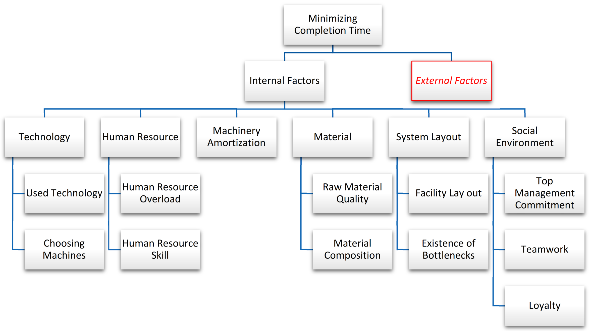
This section is divided into four main sub-sections. In the first part, the crisp weights of the internal factors will be determined. Then, using a fuzzy inference system, the fuzzy weights will be calculated. To continue, a new hybrid fuzzy–TOPSIS heuristic will be developed, which will be designed to minimize product completion time, according to the recognized factors in the previous sections. Then, some case studies will be designed using the orthogonal method (DOE) to solve the proposed method. The outcomes of this section will, then, be evaluated by several indicators and also crisp heuristic TOPSIS.

According to the findings from the literature review, the following factors must be taken into account when selecting best alternative using the proposed fuzzy–TOPSIS heuristic:

• Machine processing time;
• Maintenance program time;
• Teamwork performance;
• Material composition performance;
• Material transferring time.

The vector for the mentioned factors will be defined as [−1 −1 +1 +1 −1]. This vector, considered an input for the proposed algorithm, indicates whether maximizing a factor is desired, or it should be minimized? For example, the value for the 1st factor (machine processing time) is −1, meaning the lower value is desired.

4.1. Fuzzy Inference System

In this section, regression analysis is used to find the impact of each variable on the dependent factor (product completion time). For this purpose, linear regression in SPSS will be used.

The regression equation for each of the variables can be used to determine the weight of each factor in the next section, where a decision-making method will be proposed (

Table 3. Model summary for regression.

Model Summary b
Model	R	R Square	Adjusted R Square	Std. Error of the Estimate
1	0.860 a	0.739	0.556	10.96454

^a Predictors: (Constant), Question14, Question4, Question11, Question6, Question10, Question5, Question7, Question13, Question8, Question3, Question1, Question12, Question9, Question2; ^b Dependent Variable: Product Completion Time.

and

Table 4. Regression table for the variables of the questionnaire.

Coefficients a
Model		Unstandardized Coefficients		Standardized Coefficients	t	Sig.	95% Confidence Interval for B
		B	Std. Error	Beta			Lower Bound	Upper Bound
1	(Constant)	10.422	20.494		0.509	0.617	−32.327	53.171
	Question1	−3.025	6.057	−0.127	−0.499	0.623	−15.661	9.610
	Question2	8.218	5.931	0.471	1.386	0.181	−4.153	20.589
	Question3	−0.024	2.779	−0.002	−0.009	0.993	−5.821	5.772
	Question4	−0.428	2.918	−0.028	−0.147	0.885	−6.514	5.659
	Question5	−1.905	5.726	−0.100	−0.333	0.743	−13.848	10.038
	Question6	4.244	3.654	0.269	1.161	0.259	−3.379	11.868
	Question7	2.056	2.297	0.154	0.895	0.381	−2.736	6.847
	Question8	−0.064	4.683	−0.004	−0.014	0.989	−9.833	9.706
	Question9	−1.486	3.812	−0.094	−0.390	0.701	−9.437	6.465
	Question10	2.209	2.757	0.174	0.801	0.432	−3.542	7.960
	Question11	−2.622	3.075	−0.149	−0.853	0.404	−9.037	3.793
	Question12	11.054	5.677	0.582	1.947	0.066	−0.789	22.897
	Question13	−0.200	4.897	−0.010	−0.041	0.968	−10.416	10.016
	Question14	1.032	3.333	0.059	0.310	0.760	−5.920	7.984

^a Dependent Variable: Product Completion Time.

).

Then, using the standardized coefficients, the overall regression equation for the factors that can influence the project will be expressed as below:

Product Completion Time = −0.127Q1 + 0.471Q2 − 0.002Q3 − 0.028Q4 − 0.1Q5 + 0.269Q6 + 0.154Q7 − 0.004Q8−0.094Q9 + 0.174Q10 − 0.149Q11 + 0.582Q12 − 0.01Q13 + 0.059Q14

(2)

As shown by Equation (11), not all variables have the same impact on reducing product completion time. For example, “improving the current technology” as question 1 can significantly reduce product completion time. Most of the responders believed that due to the wrong selection of machines in their company (Q2), the completion time increased drastically. Statistical society believed that “human resources scheduling” (Q3) has less impact on reducing the production time. At the same time, “overloaded workers” (Q4) can reduce product completion time slightly. Lack of “skilled workers” (Q5) can increase product completion time significantly. People believed that “appropriate maintenance planning” (Q6) has an undoubtedly significant role in minimizing or maximizing product completion time. Experts also believed that “old machinery” (Q7) is significantly responsible for increasing product completion time. However, most responders thought the “quality of raw materials” (Q8) in their company was good enough and would not reduce product completion time.

Meanwhile, they believed that improving the “material composition” (Q9) could significantly reduce their companies’ product completion time. They also believed that “facility layout” (Q10) is responsible for decreasing product completion time strictly, and the absence of “bottleneck machines” (Q11) can decrease product completion time with the same intensity. As expected, experts believed that the most crucial factor in reducing product completion time is “top management commitment” (Q12). However, “teamwork relations” (Q14) cannot influence the dependent variable that much. However, “loyalty of human resources” (Q14) is a must for minimizing product completion time.

Using the information above, the weights of the variable clusters (machinery, maintenance, human resources, material, teamwork, and layout) can be determined for the method proposed in the next section.

The results of distributing the questionnaire to the 36 experts are gained. Cronbach’s alphas for all questions are above 0.8. The descriptive analysis is, then, performed for the questions. Using the Kolmogorov–Smirnov normal test (at 0.05), all variables are found following the normal distribution function. Then, using the Pearson Test, it is found that there are positive correlations available between variables. To continue, the regression equation is calculated, which will be helpful to determine the weight of the factor’s cluster in the next section. In the next section of Section 4, a new fuzzy–TOPSIS heuristic method will be proposed to find the best alternative among the available alternatives to minimize product completion time.

• Crisp weight of factors for the proposed hybrid TOPSIS-based heuristic

One crucial question is whether the investigated factors have the same impact on the dependent variable (product completion time)? If not, which strategy reflects the importance of factors, primarily, according to the reality of the manufacturing firms in the studied society? To answer the above questions, it is evident that the factors do not have the same value in minimizing product completion time. In Section 4.1, a regression equation is developed, according to the data gathered from the society. The regression equation can reflect the importance of each of the factors (Q(i)) on the dependent variable (Y), since the weights in the TOPSIS should be expressed between 0 and 1.

Moreover, it should become smaller in weight. In the regression equation, the coefficients of the variables have different units, so they cannot be used in a weight vector in TOPSIS. Therefore, the following calculations will be carried out to normalize the coefficients of the regression equation:

1.

Obtain regression equation:

Product Completion Time = −0.127Q1 + 0.471Q2 − 0.002Q3 − 0.028Q4 − 0.1Q5 + 0.269Q6 + 0.154Q7 − 0.004Q8 − 0.094Q9 + 0.174Q10 − 0.149Q11 + 0.582Q12 − 0.01Q13 + 0.059Q14

(3)

Find the weight of factors using:

$$w_f=\frac{{{\displaystyle \sum }}_{iϵf}{c}_i}{{{\displaystyle \sum }}_{i=1}^{14}\left|c_i\right|} \forall i \in G_f$$

(4)

where i is the counter of questions (factors); f is counter for the factor groups (f = 5); $G_f$is the factor group (machine, maintenance, material, human resources, layout); $w_i$ is the weight of the $ith$ factor, $c_i$is the coefficient of the $ith$ variable in the regression, and ${\displaystyle \sum }_{i=1}^{14}\left|c_i\right|$is the sum of the coefficients of the variables in the regression equation. Note that the absolute value of coefficients is considered to remove the effect of positive and negative elements (

Table 5. Coefficients of variables for weights.

Group	Technology		Human Resources						Maintenance		Material		Layout
Variable	Q1	Q2	Q3	Q4	Q5	Q12	Q13	Q14	Q6	Q7	Q8	Q9	Q10	Q11
Sum of Coefficients	0.127	0.471	0.002	0.028	0.1	0.582	0.01	0.059	0.269	0.154	0.004	0.094	0.174	0.149
Group Summary	0.598		0.781						0.423		0.098		0.323
Group Weights	0.269		0.351						0.190		0.044		0.145

).

The weight of factors will be calculated as follows:

Technology (Machine) Group= [C1, C2] = [0.127, 0.471]

Human Resources (Worker, Teamwork) Group= [C3, C4, C5, C12, C13, C14] = [0.002, 0.028, 0.1, 0.582, 0.01, 0.059]

Maintenance Group= [C6, C7] = [0.269, 0.154]

Material Group= [C8, C9] = [0.004, 0.094]

Layout Group= [C1, C2] = [0.174, 0.149]

Therefore, the crisp weight of the group factors will be {0.269, 0.351, 0.190, 0.044, 0.145}.

• Fuzzy weight of factors for the proposed hybrid fuzzy–TOPSIS heuristic

The weight vector calculated in the previous section can be directly used in the proposed TOPSIS-based heuristic. However, as stated in the next section, due to uncertainty available for each factor, and subsequently to the group factors, an FIS will be applied to minimize the adverse effects of uncertainty in the proposed method. Therefore, the TOPSIS-based heuristic will be developed using FIS and utilized to the fuzzy–TOPSIS heuristic.

• Fuzzy inference model

As mentioned in Section 1, uncertainty can influence the quality of solutions or even change a solution. In order to minimize the uncertainty in the decision-making process, a FIS system will be proposed.

The logic of the FIS system is to consider the response for each question along with the confidence level for the response. For this purpose, after asking each question in the questionnaire, the level of confidence about the response was also asked (Figure 7).

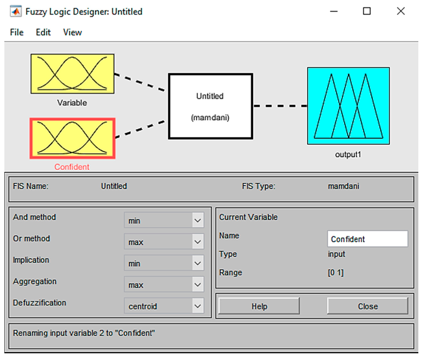
Now, let us give some information about the proposed FIS. The FIS system in this research is based on a multi-input single-output (MISO) design (Figure 8).

• Dependent variable name: Q’1, Q’2, …, Q’14.
• Inputs: {Q1, Confidence Level; Q2, Confidence Level, ..., Q14, Confidence Level}.
• Linguistic variables:
  •  Q(i) values: {Too Slow; Slow; Acceptable; Very Good; Excellent}
  •  U(i): domain of values: {0% 25% 50% 75% 100%}.
• Fuzzy engine: Mamdani rule. Note that the reason for choosing Mamdani fuzzy engine is that the fuzzy inference engine in MATLAB also uses Mamdani as the default engine in MATLAB, and therefore, it could be trusted.
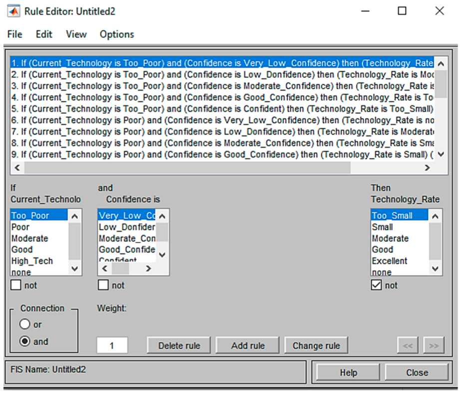
• Fuzzy rules: 25 rules for each input variable (i.e., {Q1, Confidence Level}) based on Mamdani fuzzy rule (Figure 9)).

Figure 9. A typical fuzzy diagram for a variable, according to the linguistic variables and domain of them.

Figure 9. A typical fuzzy diagram for a variable, according to the linguistic variables and domain of them.

• The logic of rules:

  $$If \left(FP is i\right) and \left(FP’ is j\right) then \left(FO is k\right)$$

  (5)

FP is a fuzzy input for variable 1; FP is a fuzzy input for variable 2, and FO is fuzzy output. i, j, and k are input parameters (based on linguistic variables) for the variables.

• Membership function:

In this research, based on the domain of the linguistic variables, trapezoidal distribution functions will be used.

A trapezoidal variable has two lower boundaries, a and upper d, as distribution parameters. Therefore, the basis of those real numbers will be in the closed distance a to d. The trapezoidal distribution has two other parameters. These two parameters called b and c represent the surfaces that indicate the beginning and end of the upper side of the trapezoid:

$$\begin{gathered} a(a<d)–lowerbound \\ b(a\le b<c)–levelstart \\ c(b<c\le d)–levelend \\ d\left(c\le d\right)–upperbound \end{gathered}$$

(6)

Accordingly, the trapezoidal distribution functions will be:

$$F_{Trapm}\left((x<X)\right)=\left\{\begin{array}{c}\left(2/d+c-a-b\right).\left(x-a\right)/\left(b-a\right);for a\le x<b\\ \left(2/d+c-a-b\right); for b\le x<c\\ \left(2/d+c-a-b\right).\left(d-x\right)/\left(d-c\right);for c\le x\le d\end{array}\right.$$

(7)

Figure 10 shows several trapezoidal graphs that are designed with different parameters. A fuzzy membership function in FIS is similar to Figure 9.

In the following, a sample for one of the variables used in FIS of the proposed TOPSIS-based heuristic will be explained in detail.

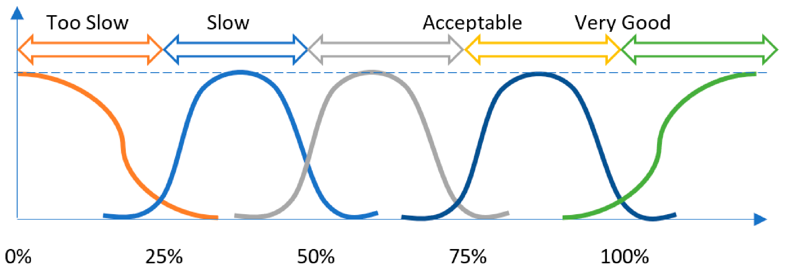
Consider “current technology,” which is asked in question 1. This question is asked in the questionnaire. The values for question is {Too Slow (0–25%); Slow (25–50%); Acceptable (50–75%); Very Good (75–100%); Excellent (100%)}. This question is considered the 1st input in the FIS.

Then, the responders ask another question: “To what extent are you sure about the response to the above question?”

This question is also considered the 2nd input of the FIS.

The outcome will be a fuzzy value that considers the “current technology” and “confidence level” (Figure 11).

In the next step, the membership functions must be defined for the input and outputs. Figure 12 indicates the fuzzy membership function for the “current technology.” As seen, using the linguistic parameters of question 1 in the questionnaire, five trapezoidal graphs are drawn for this variable. The same approach will be used for the “confidence” and “output.”

Then, the rules of the FIS will be designed based on the conditions that exist in the fuzzy system. Figure 13 shows the defined fuzzy rules for the FIS. It should be noted that due to the number of categories of the responses (Likert scale), for each of the questions (current technology and confidence), 25 (5²) rules must be defined.

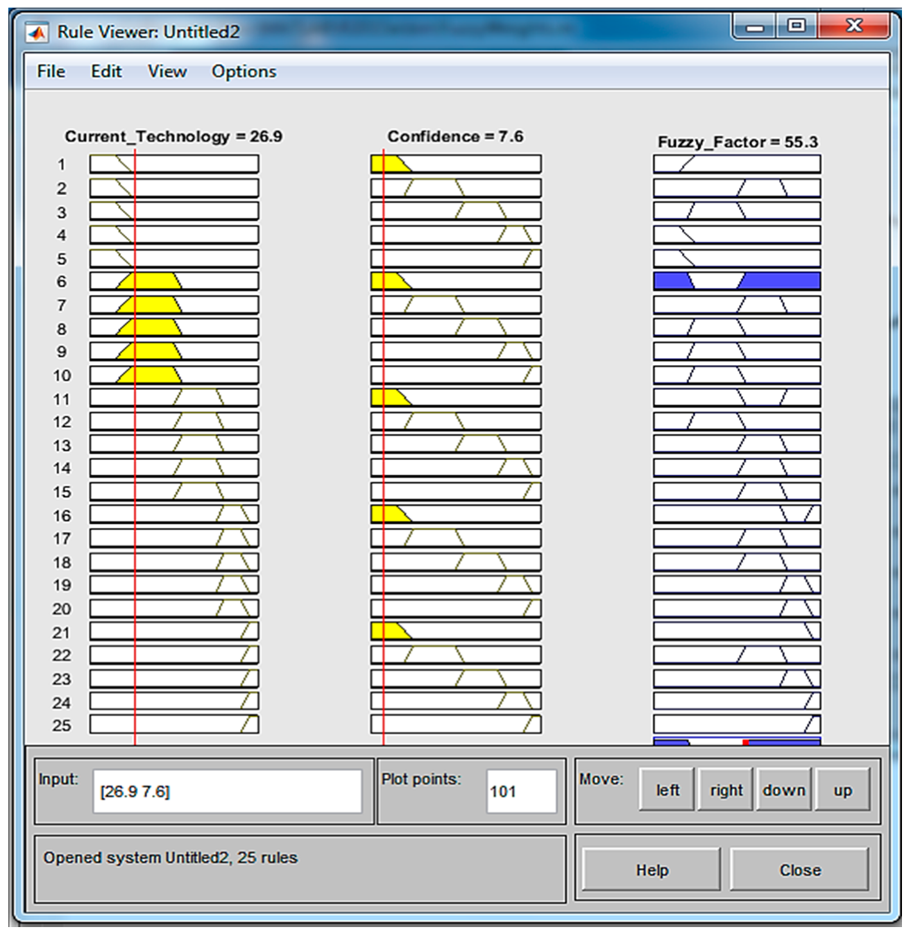
The fuzzy engine will, then, find the best options for the technology rate (Output) as the output of the FIS, according to the rules and fuzzy membership functions. This outcome is helpful to determine (estimate) the best value for “technology rate” based on the “current technology” and “confidence.” For example, Figure 14 indicates that the best option for the technology rate is 65, while current technology is 50 and confidence is also 50.

However, the same FIS proposes 37.5 for technology rate, while current technology is 35 and confidence is 90 (Figure 15).

Such influences in the technology rate are a result of the uncertainty that was obtained from the responders. Without using the fuzzy method, the impact of uncertainty cannot be considered in the calculations.

One important thing to know is the correlations between two variables (current technology and confidence) and the output variable (technology rate). Figure 16 indicates the correlations between current technology, confidence, and technology rate for the proposed method. In this figure, the higher levels of current technology and confidence at the same time will boost the technology rate.

Based on the FIS system, the crisp weights for the system are now modified and recalculated. First, a regression equation will be estimated for the confidence rates (

Table 6. Summary of the variables for the regression equation for confidence rates.

Model Summary
Model	R	R Square	Adjusted R Square	Std. Error of the Estimate
1	0.961 a	0.924	0.870	5.92885

^a Predictors: (Constant), Confidence14, Confidence5, Confidence2, Confidence11, Confidence1, Confidence6, Confidence9, Confidence7, Confidence3, Confidence13, Confidence4, Confidence12, Confidence10, Confidence8.

and

Table 7. Regression equation table for the confidence equations.

Coefficients a
Model		Unstandardized Coefficients		Standardized Coefficients	t	Sig.
		B	Std. Error	Beta
1	(Constant)	0.927	9.859		0.094	0.926
	Confidence1	0.179	3.400	0.008	0.053	0.959
	Confidence2	−5.022	2.148	−0.260	−2.338	0.030
	Confidence3	−7.377	2.480	−0.403	−2.974	0.007
	Confidence4	9.460	2.876	0.509	3.290	0.004
	Confidence5	10.303	2.639	0.437	3.905	0.001
	Confidence6	−4.101	2.859	−0.217	−1.434	0.167
	Confidence7	1.536	2.935	0.078	0.523	0.606
	Confidence8	−1.342	5.536	−0.075	−0.242	0.811
	Confidence9	−3.676	2.334	−0.220	−1.575	0.131
	Confidence10	7.719	3.794	0.498	2.035	0.055
	Confidence11	4.427	1.933	0.364	2.290	0.033
	Confidence12	−0.124	5.210	−0.007	−0.024	0.981
	Confidence13	2.403	2.452	0.133	0.980	0.339
	Confidence14	5.303	1.740	0.327	3.048	0.006

^a Dependent Variable: Product Completion Time.

).

Then, the regression equation for the confidence questions will be as follows:

Product Completion Time= 0.008Con1−0.26Con2−0.403Con3 + 0.509Con4 + 0.437Con5−0.217Con6 + 0.078Con7−0.075Con8−0.22Con9 + 0.498Con10 + 0.364Con11−0.007Con12 + 0.133Con13 + 0.327Con14

(8)

Table 8. Crisp weights of the group factors and confidence.

Group	Technology		Human Resources						Maintenance		Material		Layout
Variable	Q1	Q2	Q3	Q4	Q5	Q12	Q13	Q14	Q6	Q7	Q8	Q9	Q10	Q11
Sum of Coefficients	0.127	0.471	0.002	0.028	0.1	0.582	0.01	0.059	0.269	0.154	0.004	0.094	0.174	0.149
Group Summary	0.598		0.781						0.423		0.098		0.323
Group Weights	0.269		0.351						0.190		0.044		0.145
Group	Technology		Human Resources						Maintenance		Material		Layout
Variable	Con1	Con2	Con3	Con4	Con5	Con12	Con13	Con14	Con6	Con7	Con8	Con9	Con10	Con11
Sum of Coefficients	0.008	0.26	0.403	0.509	0.437	0.007	0.133	0.327	0.217	0.078	0.075	0.22	0.498	0.364
Group Summary	0.268		1.816						0.295		0.295		0.862
Group Weights	0.076		0.514						0.083		0.083		0.244

shows the crisp weights of the group factors and confidence, which will be used as inputs for calculating the fuzzy weights.

Using the coefficients of group factors and confidence as inputs of the proposed FIS, the fuzzy values for the weights of the fuzzy–TOPSIS heuristic will be calculated.

For example, for the technology (machine), the group factor is 0.269, while the confidence is 0.076. Using the FIS mechanism, the fuzzy weight for this factor will be 0.553 (Figure 17). As seen, uncertainty plays a crucial role in the weights of group factors in the manufacturing environment.

The rest of the fuzzy weights for the group factors are:

Fuzzy weights vector = {0.553, 0.56, 0.584, 0.602, 0.636}

(9)

In the next section, the mechanism of the proposed fuzzy–TOPSIS heuristic will be explained in detail.

4.2. A Fuzzy–TOPSIS Heuristic

In this section, a crisp TOPSIS-based heuristic will be proposed first. Then, to show the role of uncertainty in the manufacturing environment, a fuzzy–TOPSIS heuristic will be proposed. Both methods are designed to generate alternatives, according to the information about machinery, required maintenance, material, workers, and shop size (layout). The aim is to find the best alternative that minimizes product completion time.

The outcomes of the proposed fuzzy–TOPSIS heuristic (as the primary method of the research) shall answer the following questions:

• How many products should be manufactured?
• Which type of materials should be used?
• Which machines should be assigned?
• What are the best locations for the machines?
• Which operators shall be used?
• What maintenance should be applied?

For this purpose, the following matrixes shall be defined as inputs of the proposed heuristic:

• Product demand;
• Product–machine requirement;
• Machine capacity;
• Material–machine processing time;
• Technology material;
• HR availability;
• HR skill;
• HR cluster;
• Machine-maintenance type;
• Machine maintenance period;
• Machine maintenance time;
• Machine distance.

The following indices are defined to clarify the domain of variables, parameters, and matrixes:

• i: type of product;
• j: type of material;
• k: type of machine;
• o: type of operator;
• s: operator skill level;
• t: time slot;
• m: maintenance type.

Accordingly, the input matrices that will be used in the proposed method will be defined as follows:

(1)

“Number_of_Factors” indicates the number of factors that must be considered in a problem. According to the 1st part of Section 4, product completion time, maintenance time, operator processing time, material composition processing time, and material transferring time are the factors to be considered in all examples.

(2)

“Number_of_Alternatives” allows the decision maker to control the number of alternatives generated by the proposed heuristic.

(3)

Vector_of_Factors: indicates that whether maximizing (+1) or minimizing (−1) of a factor is desired.

(4)

“Weight_of_Factors” indicates the importance of the factors. The value for this matrix is taken from the questionnaire and can reflect the fundamental idea of experts in this field.

(5)

“Length_of_Shop” indicates the length of a shop.

(6)

“Width_of_Shop” indicates the width of a shop.

(7)

“Product_Demand” shows how many products must be manufactured through a planning horizon.

(8)

“Available_Time” shows the available time in a production horizon and can be considered a threshold value to accept or reject a generated alternative by the supervised algorithm.

(9)

“Number_of_Operations” shows the number of operation (machines) that is required for producing a product.

(10)

“Product_Machine_Sequence” shows the sequence of operations to be carried out, respectively.

(11)

“Machine_Type_Alternative” shows the available number of each machine type.

(12)

“Machine_Processing_Time” indicates the processing time required for each machine type to complete a service. The processing time for parallel machines (of an identical type) could differ, according to their brand, age, and amortization.

(13)

“Reliability_Percentage_of_Machines”: The reliability of a machine indicates the possibility of working without failure. Therefore, the value 1-reliability will be added to the machine processing time.

(14)

“Machine_Sequence” indicates the ID for each machine and will be used in the calculation process.

(15)

“Machine_Maintenace_Frequency” represents the number of times that a machine requires maintenance in a period.

(16)

“Machine_Maintenace_Time” indicates the maintenance time for each machine, according to its type and ID.

(17)

“Human_Skill_Alternative” indicates the number of workers for a specific operation.

(18)

“Human_Processing_Skill,” a value between 0 and 2 expresses the members of this matrix. If a worker’s skill is 1, he/she can perform a task in a standard time. Similarly, if a human worker’s skill is 0.98, he/she can perform a task 2% quicker than usual.

(19)

“Number_of_Required_Material” indicates the type of raw materials that are required to complete a product.

(20)

“Types_of_Material” shows the number of alternatives available for each material type (for example, two different brands or different compositions for raw material).

(21)

“Material_Processing_Time” is a matrix expressed by 0 and 2. If the element is 1, the material quality is standard and does not affect the processing time. However, if an element is more than 1 (for example, 1.05), it means that the raw material needs 5% more time than the standard processing time expressed by the Machine_Processing_Time matrix.

(22)

“Number_of_Layouts_To_Be_Considered” allows the decision maker to choose how many layouts should be generated by the algorithm. The higher number of layouts increases the solving time.

(23)

“Unit_Material_Transferring_cost” indicates the time of material transferring of one unit of raw material and is expressed according to the linear distance between machines in a layout.

• The mechanism of the proposed fuzzy–TOPSIS heuristic

The following flowchart indicates the mechanism of the proposed heuristic in detail (Figure 18).

4.3. Design of Experiments

In this section, several case studies that consider different conditions must be solved. For this purpose, an orthogonal method will be used to design the case studies. Using DOE is also helpful for evaluating whether the proposed method can solve all different conditions successfully? On the other hand, DOE can also help to find which elements are more critical. DOE has been widely applied in the research studies where a new method was proposed. In this research, the same strategy that has been applied by Delgoshaei et al. for evaluating their proposed hybrid Tabu search and ant colony optimization method for scheduling problems will be used. For this purpose, the orthogonal method will be designed using SPSS. The aim is to design various problems that will be solved by the proposed algorithm, where all possible conditions will be taken into account.

The proposed method has five main factors: machinery (and maintenance); worker; material; number of layouts; number of alternatives.

The mentioned factors are defined in the SPSS orthogonal design first (Figure 19).

Then, three levels will be considered for each factor, which is considered, according to small-, medium-, and extensive-sized case studies (Figure 20).

Then, SPSS will design an orthogonal case with the mentioned factors and levels (Figure 21).

In continuation, SPSS will design 16 plan cards for the mentioned DOE (

Table 9. Plan cards that are designed by orthogonal design using SPSS.

Card List
	Card ID	Machine	Worker	Material	Layout	Alternatives
1	1	10	10	3	50	1000
2	2	10	10	5	20	5000
3	3	2	10	5	20	2000
4	4	20	20	5	100	1000
5	5	2	5	2	20	1000
6	6	2	5	3	100	1000
7	7	20	20	3	20	5000
8	8	2	20	2	50	5000
9	9	2	20	3	20	2000
10	10	10	20	2	20	1000
11	11	20	20	2	50	2000
12	12	10	10	2	100	2000
13	13	2	5	5	50	1000
14	14	20	20	2	20	1000
15	15	10	10	5	20	1000
16	16	2	10	2	100	5000

). Each of the experiments will be solved in the next section to see if the proposed method can solve all the case studies in various conditions.

4.4. Verifying the Proposed Algorithm (Solving Experiments Gathered from the Literature)

In this section, using the orthogonal design in the previous section, several case studies will be solved to verify the proposed algorithm’s functionality in different conditions. The case studies are designed in such a way that the various range of parameters is taken into account. In this section, each of the case studies will be solved by the proposed algorithm in MATLAB. The outcomes of the case studies are shown in

Table 10. Results of solving numerical experiments using the proposed hybrid fuzzy-TOPIS heuristic.

No.	Machine	Worker	Material	Layout	Alternatives	Best Alternative	Product Processing Time	Maintenance Time	Operator Processing Time	Material Transferring Time	Best Observed CL	Worst Observed CL	Solving Time (Second)
1	10	10	3	50	1000	449	30,264	296	0.517	16.000	0.989	0.040	0.699
2	10	5	5	20	5000	2383	29,678	296	0.522	19.000	0.998	0.013	1.351
3	2	10	5	20	2000	1535	6600	63	0.931	1.000	0.993	0.008	0.285
4	20	20	5	100	1000	581	59,348	450	0.960	71.000	0.965	0.016	2.680
5	2	5	2	20	1000	490	6600	50	0.931	1.000	0.995	0.016	0.165
6	2	5	3	100	1000	669	6600	50	0.931	1.000	0.996	0.014	0.162
7	20	5	3	20	5000	2898	59,348	450	0.960	69.000	1.000	0.006	3.385
8	2	20	2	50	5000	4483	6600	50	0.884	1.000	1.000	0.000	0.795
9	2	20	3	20	2000	1556	6600	50	0.884	1.000	1.000	0.000	0.280
10	10	20	2	20	1000	723	29,674	225	1.744	29.000	0.986	0.007	0.183
11	20	5	2	50	2000	1348	59,352	450	0.960	70.000	1.000	0.006	2.863
12	10	5	2	100	2000	854	29,678	297	0.522	17.000	0.998	0.034	0.826
13	2	5	5	50	1000	468	6600	50	0.931	1.000	0.995	0.000	0.161
14	20	10	2	20	1000	925	59,348	450	0.960	82.000	1.000	0.022	2.710
15	2	5	2	20	1000	459	29,674	225	2.050	34.000	0.925	0.034	0.186
16	2	10	2	100	5000	4921	6600	63	0.931	1.000	1.000	0.009	0.782

. As seen in each case, the best alternative that is observed is shown.

Moreover, the best machine selection, maintenance plan, workers, material composition, and layout will be shown. The performance of the proposed algorithm that indicates the quality of the gained solutions is shown in Section 4.5. In the next section, and to give detailed information on the method, case study number 3 in Table 10 will be explained.

After solving a case study, the outcomes will be presented in the following format:

Best scenario: machine/maintenance/teamwork/material/layout.

Each of the elements of the above structure will be represented as a matrix. To continue, each of the matrices mentioned above will be explained.

Suppose in a manufacturing company, three operations must be done sequentially to complete a product. Each row of the machine processing time shows the number of available machines for each operation and the processing time for each operation.

Machine: the machine processing time matrix indicates the required time for processing a task (or serving a service) using a specific machine type. For example:

Machine_Processing_Time = [10 0 0; 12 14 11; 13 12 0]

It shows that for performing service 1, there is only one machine available (as there is only one element in the 1st row) that requires 10 s to complete one task. In contrast to the 2nd operation, there are three machines available (suppose three welding machines), where performing the 2nd operation with the 1st machine needs 12 s, the 2nd machine needs 14 s, and the 3rd machine needs 11 s.

The set of selected machines and standard time (including the reliability) required to complete a product will be represented in the method’s output. For instance:

Best_Proceesing_Time = 11.5000 11.9900 18.8500

The above matrix shows that the 1st machine type 1 is selected to perform the first operation, requiring 11.5 s. The 3rd machine type 2 is selected for performing the 2nd service, and the 1st machine type 3 is selected for operating the 3rd operation.

Maintenance program: maintenance matrix will show the time required for the maintenance services if a selected number of machines are used.

As the method’s input, two matrices are defined, where the 1st matrix shows the frequency of maintenance required for each machine in a manufacturing period, and the 2nd matrix shows the required time for performing a maintenance task for each machine.

Machine_Maintenace_Frequency = [1 0 0; 2 4 1; 3 1 0]

Machine_Maintenace_Time = [100 0 0; 120 140 110; 130 120 0]

The output of the method shows the total maintenance time that is required for each machine type. For example:

Best_Maintenance_Time = 100 110 390

The above matrix shows 100 min required for machine type 1 (which provides the 1st service), 110 min for performing maintenance activities for machine type 2, and 390 min for performing maintenance for machine type 3.

Operator (teamwork): as the input of the method, the following matrices will be entered:

The human skill alternative matrix indicates the number of skilled workers who can work with a machine (perform a technical task). For example:

Human_Skill_Alternative = [2 3 3]

It shows that there are two operators available to assign for performing task 1, while there are three workers for performing the 2nd task.

The human processing skill matrix indicates the spare time that will be added (or reduced) to the standard processing time due to a lack (or addition) of skill. For example, the 1st operator’s value is 1.01, which means that this operator is slightly slower than a regular standard time for operating task 1, while the 2nd operator for performing task 2 is a super-fast operator who can perform a task faster than usual (0.94).

Human_Processing_Skill = [1.01 0.99 0; 1.2 0.94 0.99; 1.1 1.12 1.09]

The output of the method will be shown as the following:

Best_Human_Skill_Time = 1.0100 0.9900 1.0900

The above matrix has two meanings. The first is which operator is selected for performing a task. For example, the 1st and third operators type 1, 2, and 3 are selected for tasks 1, 2, and 3, respectively. Moreover, this matrix shows the best team combination that can perform the tasks with the highest performance.

Material: as an input, three matrices describe the materials used for completing a product.

The amount of required materials shows the type of raw materials required to complete a product (i.e., two types of raw materials).

The types of material show the number of alternatives that are available for each type of material. For example, [2 3] shows that for the 1st material, there are two options (i.e., two brands), and for the 2nd material, there are three options available.

Material processing time indicates the extra time required to perform a service due to the raw materials’ low (high) quality compared to the standard time.

Material Processing Time = [1.02 1.03 0; 1.02 1.01 0.98]

For example, 1.0 shows that the 1st brand of material type 1 (1.02) has better quality than the second brand (1.03). However, both materials need more time than normal time. The output of the method would be:

Best_Material_Composition = 1.0200 0.9800

For the 1st type of raw materials, the 1st brand is more desired, and for the second, the 3rd brand is more desired.

Layout: The proposed heuristic method is capable of obtaining the length and width of a shop and finding the best location of the machines, according to the material transferring cost (or time). For choosing the best location, the algorithm also considers the sequence of the materials for producing a product. For example, the following example shows that the shop has enough space to locate 12 (4 × 3) machines.

Length_of_Shop = 3

Width_of_Shop = 4

Another critical input that increases the decision-making process’s performance is the number of layouts to be considered. This input allows the decision maker to increase or decrease the number of alternatives. The idea behind this decision is that in most cases, the number of possible alternatives for locating machines inside a small-scale shop is too much, and therefore, the processing time could be influenced by the enormous number of layouts, which is not necessary.

Therefore, we decided to let the decision maker choose the number of layouts to be considered.

Number_of_Layouts_Tobeconsidered = 10

Finally, the last input is the material transferring penalty, which can be expressed as time or cost. It depends on the type of material. For example, in the following matrix, the material transferring cost for the 1st raw material is 10 RM, while the 2nd raw material is 20 RM.

Unit_Material_Transferring_cost = [10 20]

The outcome of the proposed method shows the best layout for locating a series of machines, according to the material consequence and machines. For example, for a case study, the following layout shows that the best layout is to locate the machines consecutively as the OPC for producing the product (1 2 3), which shows that raw materials visit machines 1, 2, and 3, respectively.

Best_Block_Position_in_Shop_Alternative = 1 2 3 0 0 0 0 0 0 0 0 0

4.5. Measuring the Performance of the Proposed Algorithm

In order to assess the performance of the proposed method, several indicators are defined as shown below:

• Solving strength;
• Generating scenario capability;
• The ability to generate scenarios with the lowest uncertainty;
• Solving time
• Comparing the hybrid fuzzy–TOPSIS heuristic with crisp heuristic TOPSIS;
• The ability to solve all problem types.

The results of 16 experiments gained by solving the proposed hybrid fuzzy–TOPSIS heuristic showed that the proposed method could solve all experiments (100%) and show the best alternative with the lowest product completion time.

$$Validating·Index=\frac{Number of Solved Cases without error}{Number of Orthogonal Designed Cases}·100=\frac{16}{16}\times 100=100\%$$

(10)

Therefore, the results indicated that the proposed method could be safely used for the various conditions in real industries.

• The ability to elect the alternative with the lowest product completion time

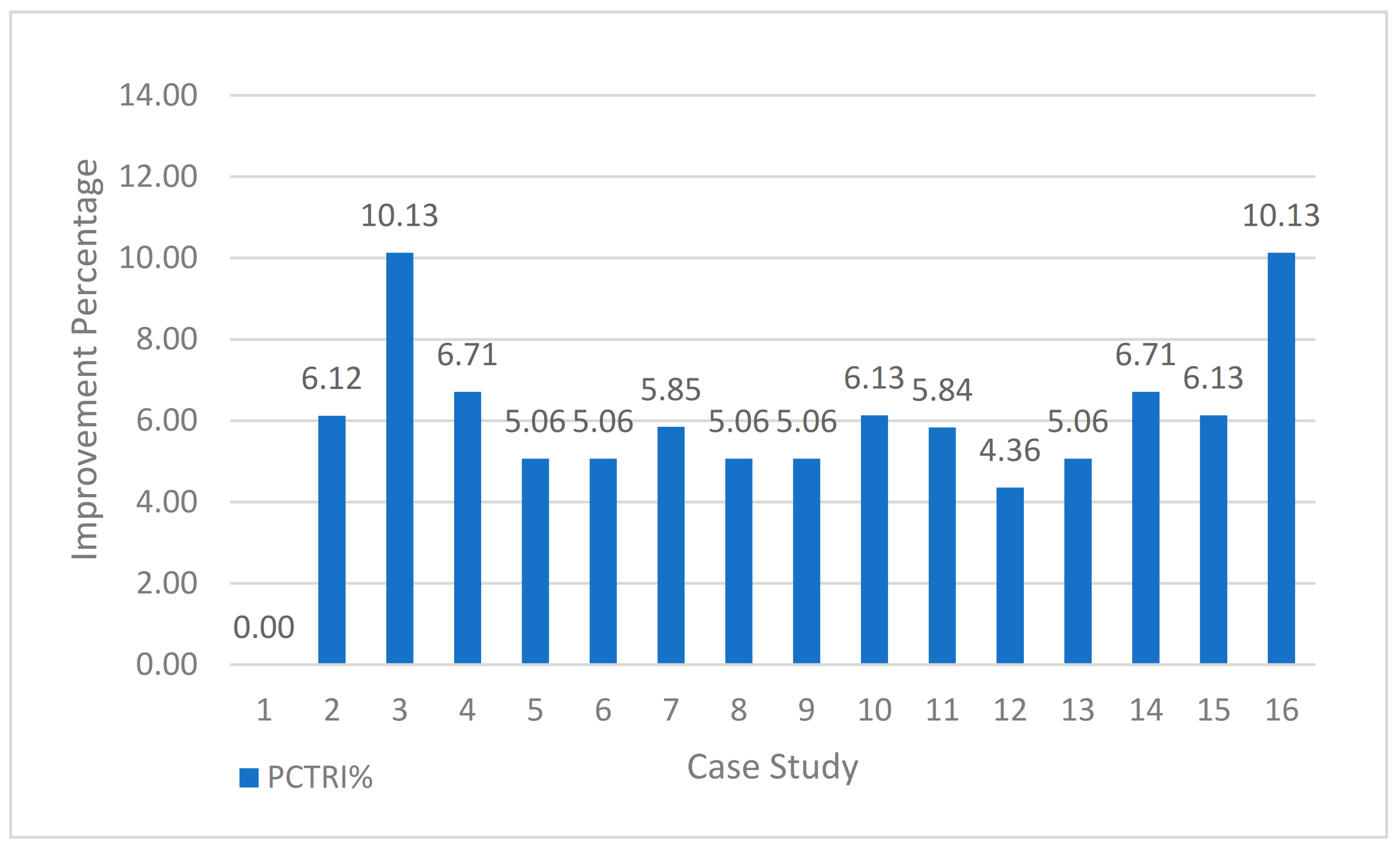
This research aims to design a method to choose the alternative with the lowest product completion time. Therefore, it is essential to check whether the proposed hybrid fuzzy–TOPSIS heuristic can choose the best alternative with the lowest product completion time among the other alternatives. For this purpose, an indicator is developed to check whether the proposed method could help elect the alternative with the lowest product completion time.

$$Lowest Product Completion Time Indicator=\left[\frac{\sum Case Studies with Lowest Product Completion Time}{Number of Studied Cases}\right]·100=100\%$$

(11)

• The performance of the proposed method

One crucial question is to what percentage the proposed method can select the alternatives with the lowest product completion time. In other words, PCTRI% shows how much percentage using the proposed algorithm is helpful to select the alternative with the lowest risk factor (

Table 11. The results of PCTRI% for studies solved by the proposed method.

Row	Worst Processing Time in Alternatives	Best Processing Time in Alternatives	PCT that Reported by the Proposed Method	PCTRI%
1	30,264	30,264	-	0.00
2	31,612	29,678	✓	6.12
3	7344	6600	✓	10.13
4	63,616	59,348	✓	6.71
5	6952	6600	✓	5.06
6	6952	6600	✓	5.06
7	63,034	59,348	✓	5.85
8	6952	6600	✓	5.06
9	6952	6600	✓	5.06
10	31,612	29,674	✓	6.13
11	63,030	59,352	✓	5.84
12	31,030	29,678	✓	4.36
13	6952	6600	✓	5.06
14	63,616	59,348	✓	6.71
15	31,612	29,674	✓	6.13
16	7344	6600	✓	10.13

).

$$PCTRI{\%}^{*}=\left[\frac{Alternative With Lowest PCT}{Alternative With Highest PCT}\right]·100$$

(12)

$* PCTRI: Product Completion Time Reduced Index.$

As seen in Figure 22, the algorithm can choose the alternative with the lowest product completion time in all cases.

• Solving Time

The solving time for the case studies is another critical factor that must be considered to evaluate the proposed method’s performance. For this purpose, the solving time of the studied cases is drawn and represented by Figure 23.

As seen, the hybrid Fuzzy–TOPSIS heuristic algorithm can solve the orthogonal cases in a range between 0.161 and 3.385 s, depending on the size of the cases. The solving time for all case studies is reasonable.

• Comparing the functionality hybrid fuzzy–TOPSIS heuristic algorithm with crisp heuristic TOPSIS

One crucial question to be answered is whether the crisp heuristic TOPSIS can report the same results. In other words, can the uncertainty cause changes in the outcome of the selecting process? To answer this question, the 10 experiments with different conditions will be solved by both the proposed fuzzy–TOPSIS heuristic and crisp heuristic TOPSIS. The aim is to compare the results and see what the difference between the gained results is. The results of solving the new 10 case studies that are solved by crisp and fuzzy–TOPSIS heuristic are represented by

Table 12. Result of comparing crisp TOPSIS heuristic with the fuzzy–TOPSIS heuristic method.

No.	Number of Alternatives	Crisp TOPSIS Heuristic		Fuzzy–TOPSIS Heuristic		$\mathbf{\Delta }\mathit{C}\mathit{L}’\mathit{i}/\mathbf{\Delta }\mathit{C}\mathit{L}\mathit{i}$	Crisp Solving Time	Fuzzy Solving Time
		Worst Fuzzy CL	Best Crisp CL	Worst Fuzzy CL’	Best Fuzzy CL’
1	100	0.086	0.952	0.054	0.966	1.054	0.015	0.015
2	500	0.000	0.947	0.000	0.953	1.006	0.047	0.046
3	1000	0.040	1.000	0.057	1.000	0.982	0.108	0.107
4	1000	0.009	0.994	0.006	0.992	1.001	0.101	0.098
5	1000	0.000	1.000	0.000	1.000	1.000	0.104	0.109
6	1000	0.015	1.000	0.035	1.000	0.980	0.101	0.104
7	1000	0.000	1.000	0.000	1.000	1.000	0.167	0.170
8	2000	0.000	1.000	0.000	1.000	1.000	0.218	0.214
9	2000	0.047	1.000	0.023	1.000	1.025	0.219	0.215
10	5000	0.026	1.000	0.015	1.000	1.011	0.630	0.645

.

It is found that that the outcomes of the proposed hybrid fuzzy–TOPSIS heuristic are significantly different from the crisp heuristic TOPSIS, which means that uncertainty can cause considerable differences in CL ranges (range of ranking alternatives from ideal positive and negative solutions). Therefore, using the fuzzy–TOPSIS method is strongly recommended for choosing production alternatives in a manufacturing environment.

• Minimum variation (MV)

In addition to the indicators mentioned above, an important indicator can measure the proposed method’s performance. Laue et al. [67], in their research, used minimum variation (MV) and total deviation (TD) as indicators that can evaluate the performance of their method. In this research, the same concept is inspired but changed a little to fit the methodology of this research. For this purpose, the pairwise comparison between the results that are gained by solving crisp and fuzzy methods will be calculated, according to the following formula:

$${\phi }_{ij}=\frac{\Delta C{L}^{\prime }i}{\Delta CLi}=\frac{\mathrm{Best} \mathrm{Fuzzy} {\mathrm{CL}}^{\prime }-\mathrm{Worst} \mathrm{Fuzzy} {\mathrm{CL}}^{\prime }}{\mathrm{Best} \mathrm{Crisp} \mathrm{CL}-\mathrm{Worst} \mathrm{Fuzzy} \mathrm{CL}} ; \mathrm{for} i\in n$$

(13)

where n indicates the number of experiments. $V_{ij}{}^u$ is the vector of the values that can be gained by comparing the pairwise comparison between the crisp and fuzzy methods and can be calculated according to the following formula:

$$V_i{}^u=\left\{\begin{array}{c}\begin{array}{cc}1& if {\phi }_{ij}>1 \end{array}\\ \begin{array}{c}\begin{array}{cc}0.5& {\phi }_{ij}=1\end{array}\\ \begin{array}{cc}0& {\phi }_{ij}<1\end{array}\end{array}\end{array}\right.$$

(14)

The minimum variation formula for this research can be calculated according to the following formula:

$$MV=\sum _i^n\frac{V_i{}^u}{n-1}$$

(15)

The result of calculating the MV indicator for the values in Table 12 is 0.72. Considering the aim of the proposed method, which is finding the best and worst alternatives in terms of product completion time, the gained value (0.72) can be considered a significant value.

However, crisp TOPSIS heuristic is slightly faster in solving case studies (Figure 24).

After solving the case studies, the following results were gained (

Table 13. Results of comparing the crisp heuristic TOPSIS with the proposed fuzzy–TOPSIS heuristic.

Row	Crisp Heuristic TOPSIS	The Proposed Hybrid Fuzzy–TOPSIS Heuristic
1	The crisp heuristic TOPSIS could not consider uncertainty	The proposed method considered uncertainty in its calculation
2	The crisp heuristic TOPSIS is slightly faster	The proposed method speed is moderate
3	The crisp heuristic TOPSIS could not generate alternatives using manufacturing systems input	The proposed fuzzy–TOPSIS heuristic could generate alternatives using manufacturing systems input
4	Weight of factors in the crisp heuristic TOPSIS is crisp	Weight of factors in the proposed method is fuzzy
5	The crisp heuristic TOPSIS can only select the best alternative	The proposed method could report the best machine selection, maintenance plan, worker team, material composition, and facility layout

):

5. Conclusions

This research focused on internal factors in minimizing product completion time in a manufacturing firm. The aim is to recognize the factors that can influence product completion time. For this purpose, several factors are outlined from the literature review as well as the Delphi method. For this purpose, 14 factors are identified and clustered into five main groups: technology (machinery), maintenance, workers (skill, teamwork), material, and layout.

Then, a questionnaire was designed to find the impact of the recognized factors on product completion time (as the dependent variable of the research). The questionnaire was, then, distributed to some experts, according to the central limit theorem.

Then, a series of statistical analyses have been done to figure out the correlations between variables and their impact on the dependent variable. It is found that human resources (0.351), technology (0.269), maintenance (0.19), layout (0.145), and material (0.044) have the greatest role in minimizing (or maximizing) product completion time. It is also argued that due to the uncertainty in the manufacturing environment, a fuzzy system inference must be designed and applied to consider the uncertainty in determining the correct weights for the regression equation. A Mamdani rule has been applied for the proposed fuzzy inference system. It is found that uncertainty can significantly have an impact on product completion time minimization. After applying the fuzzy inference, the modified fuzzy weights were found: 0.553, 0.56, 0.584, 0.602, and 0.636 for machinery, human resources, maintenance, material, and layout.

In the second section of the research, a fuzzy–TOPSIS heuristic was proposed for generating and finding the best alternative in a manufacturing system to minimize product completion time. The proposed method is capable of generating several alternatives, according to the inputs of the model.

Then, using SPSS, an orthogonal design is designed to generate some case studies to be solved by the proposed fuzzy–TOPSIS heuristic. After solving the case studies, the method’s performance was evaluated by four indicators: validating index, lowest product completion time indicator, product completion time reduced index (PCTRI), and processing time. Validating index: The proposed method could solve 100% of the orthogonal case studies. Lowest product completion time indicator: The proposed method could find the minimum product completion time for all the studied cases. Product completion time reduced index (PCTRI): This presents outcomes of comparing the best and worst alternatives for each case study; the proposed method could minimize product completion time in the range 0% to 10.13%. Processing time: The results indicated that the proposed method could solve all case studies in less than 6 s. However, the proposed fuzzy–TOPSIS heuristic is significantly slower than classic TOPSIS. This low solving speed proposed in the method could generate the alternatives before finding the best alternative. However, the speed of the crisp and fuzzy heuristics are approximately the same.

Moreover, the performance of the proposed hybrid method is compared with the crisp heuristic TOPSIS. It is found that, while crisp heuristic TOPSIS is relatively faster than the proposed fuzzy–TOPSIS hyper, it cannot consider the uncertainty, and thus, its result is not applicable for this research.

While conducting the research, many gaps are found that can be considered recommendations for future research studies. It is recommended to conduct another study, where external factors that can influence product completion time in manufacturing systems are considered. It is suggested to develop software using the outcomes of this research, which enables engineers in the accurate world to use the proposed method in this research. It is suggested to use different MADAM methods such as VICOR and AHP and compare the performance of the proposed method in this research with them. One can develop a mathematical model using the regression equation used in this research and solve the model using optimization, heuristic, or metaheuristic methods. One can develop a multi-agent model to study the role of different agents in a manufacturing system (i.e., owners, suppliers, top management, engineers, workers, and stockholders) in minimizing product completion time. It is recommended to develop a dynamic model to investigate the impact of selecting this research’s different alternatives (production strategies).

References

1. Xu, R.; Chen, H.-P.; Shao, H.; Wang, S.-S. Two kinds of ant colony algorithms to minimize the total completion time for batch scheduling problem. Comput. Integr. Manuf. Syst. 2010, 16, 1255–1264. [Google Scholar]
2. Irdem, D.F.; Kacar, N.B.; Uzsoy, R. An exploratory analysis of two iterative linear programming—simulation approaches for production planning. IEEE Trans. Semicond. Manuf. 2010, 23, 442–455. [Google Scholar] [CrossRef]
3. Ramezanian, R.; Rahmani, D.; Barzinpour, F. An aggregate production planning model for two phase production systems: Solving with genetic algorithm and tabu search. Expert Syst. Appl. 2012, 39, 1256–1263. [Google Scholar] [CrossRef]
4. Shah, N.K.; Ierapetritou, M.G. Integrated production planning and scheduling optimization of multisite, multiproduct process industry. Comput. Chem. Eng. 2012, 37, 214–226. [Google Scholar] [CrossRef]
5. Ning, Y.; Liu, J.; Yan, L. Uncertain aggregate production planning. Soft Comput. 2013, 17, 617–624. [Google Scholar] [CrossRef]
6. Wang, S.-C.; Yeh, M.-F. A modified particle swarm optimization for aggregate production planning. Expert Syst. Appl. 2014, 41, 3069–3077. [Google Scholar] [CrossRef]
7. Díaz-Madroñero, M.; Mula, J.; Peidro, D. A review of discrete-time optimization models for tactical production planning. Int. J. Prod. Res. 2014, 52, 5171–5205. [Google Scholar] [CrossRef]
8. Gansterer, M.; Almeder, C.; Hartl, R.F. Simulation-based optimization methods for setting production planning parameters. Int. J. Prod. Econ. 2014, 151, 206–213. [Google Scholar] [CrossRef]
9. Kodialam, M.S.; Lakshman, T.V.; Mukherjee, S.; Chang, H.; Lee, M.J. Scheduling in MapReduce-like systems for fast completion time. In Proceedings of the 2011 Proceedings IEEE INFOCOM, Shanghai, China, 10–15 April 2011. [Google Scholar]
10. Rossi, T.; Pozzi, R.; Pero, M.; Cigolini, R. Improving production planning through finite-capacity MRP. Int. J. Prod. Res. 2017, 55, 377–391. [Google Scholar] [CrossRef]
11. Yang, L.; Li, J.; Hackney, P.; Chao, F.; Flanagan, M. Manual task completion time estimation for job shop scheduling using a fuzzy inference system. In Proceedings of the 2017 IEEE International Conference on Internet of Things (iThings) and IEEE Green Computing and Communications (GreenCom) and IEEE Cyber, Physical and Social Computing (CPSCom) and IEEE Smart Data (SmartData), Exeter, UK, 21–23 June 2017; pp. 139–146. [Google Scholar]
12. Żywicki, K.; Osiński, F.; Wichniarek, R. Methodology of Estimating Manufacturing Task Completion Time for Make-to-Order Production. In Proceedings of the International Conference on Innovation, Engineering and Entrepreneurship, Guimaraes, Portugal, 27–29 June 2018; Springer: Berlin/Heidelberg, Germany, 2018; pp. 377–383. [Google Scholar]
13. Wang, J.; Yang, J.; Zhang, J.; Wang, X.; Zhang, W. Big data driven cycle time parallel prediction for production planning in wafer manufacturing. Enterp. Inf. Syst. 2018, 12, 714–732. [Google Scholar] [CrossRef]
14. Rauch, E.; Dallasega, P.; Matt, D.T. Complexity reduction in engineer-to-order industry through real-time capable production planning and control. Prod. Eng. 2018, 12, 341–352. [Google Scholar] [CrossRef]
15. Rubaiee, S.; Yildirim, M.B. An energy-aware multiobjective ant colony algorithm to minimize total completion time and energy cost on a single-machine preemptive scheduling. Comput. Ind. Eng. 2019, 127, 240–252. [Google Scholar] [CrossRef]
16. Huang, J.; Chang, Q.; Arinez, J. Product Completion Time Prediction Using A Hybrid Approach Combining Deep Learning and System Model. J. Manuf. Syst. 2020, 57, 311–322. [Google Scholar] [CrossRef]
17. de Curs, E.S.; Ouahman, A.A.; Ibourk, A. Integrated Model Based on Extended Fuzzy AHP and Criticality Analysis for Risk Assessment in Customs Supply Chain: A Perspective from Morocco. Int. J. Ind. Eng. Theory Appl. Pract. 2020, 27, 181–208. [Google Scholar]
18. Fischer, K.A.; Knipfer, I.W.; Knodel, K.D.; MacPherson, M.J. Real-Time Predictive Time-to-Completion for Variable Configure-to-Order Manufacturing. U.S. Patent No. 7,647,130, 12 January 2010. [Google Scholar]
19. Erol, R.; Sahin, C.; Baykasoglu, A.; Kaplanoglu, V. A multi-agent based approach to dynamic scheduling of machines and automated guided vehicles in manufacturing systems. Appl. Soft Comput. 2012, 12, 1720–1732. [Google Scholar] [CrossRef]
20. Gen, M.; Lin, L. Multiobjective evolutionary algorithm for manufacturing scheduling problems: State-of-the-art survey. J. Intell. Manuf. 2014, 25, 849–866. [Google Scholar] [CrossRef]
21. Kapanoglu, M.; Alikalfa, M.; Ozkan, M.; Parlaktuna, O. A pattern-based genetic algorithm for multi-robot coverage path planning minimizing completion time. J. Intell. Manuf. 2012, 23, 1035–1045. [Google Scholar] [CrossRef]
22. Li, K.; Leung, J.-T.; Cheng, B.-Y. An agent-based intelligent algorithm for uniform machine scheduling to minimize total completion time. Appl. Soft Comput. 2014, 25, 277–284. [Google Scholar] [CrossRef]
23. Angius, A.; Horváth, A.; Colledani, M. Moments of accumulated reward and completion time in Markovian models with application to unreliable manufacturing systems. Perform. Eval. 2014, 75, 69–88. [Google Scholar] [CrossRef]
24. Mokhtari, H.; Salmasnia, A. An evolutionary clustering-based optimization to minimize total weighted completion time variance in a multiple machine manufacturing system. Int. J. Inf. Technol. Decis. Mak. 2015, 14, 971–991. [Google Scholar] [CrossRef]
25. Li, Z.; Tang, Q.; Zhang, L. Minimizing energy consumption and cycle time in two-sided robotic assembly line systems using restarted simulated annealing algorithm. J. Clean. Prod. 2016, 135, 508–522. [Google Scholar] [CrossRef]
26. Costa, A.; Cappadonna, F.A.; Fichera, S. Minimizing the total completion time on a parallel machine system with tool changes. Comput. Ind. Eng. 2016, 91, 290–301. [Google Scholar] [CrossRef]
27. Smutnicki, C. Minimizing cycle time in manufacturing systems with additional technological constraints. In Proceedings of the 2017 22nd International Conference on Methods and Models in Automation and Robotics (MMAR), Miedzyzdroje, Poland, 28–31 August 2017; pp. 463–470. [Google Scholar]
28. Chen, X.-J.; Hu, J.-L.; Zhou, Q.-L.; Politis, C.; Sun, Y. An automatic optimization method for minimizing supporting structures in additive manufacturing. Adv. Manuf. 2020, 8, 49–58. [Google Scholar] [CrossRef]
29. Delgoshaei, A.; Ali, A. Review evolution of cellular manufacturing system’s approaches: Human resource planning method. J. Proj. Manag. 2019, 4, 31–42. [Google Scholar] [CrossRef]
30. Aryanezhad, M.; Deljoo, V.; Mirzapour Al-e-hashem, S. Dynamic cell formation and the worker assignment problem: A new model. Int. J. Adv. Manuf. Technol. 2009, 41, 329–342. [Google Scholar] [CrossRef]
31. Süer, G.A.; Kamat, K.; Mese, E.; Huang, J. Minimizing total tardiness subject to manpower restriction in labor-intensive manufacturing cells. Math. Comput. Model. 2013, 57, 741–753. [Google Scholar] [CrossRef]
32. Delgoshaei, A.; Ali, A. An applicable method for scheduling temporary and skilled-workers in dynamic cellular manufacturing systems using hybrid ant colony optimization and tabu search algorithms. J. Ind. Prod. Eng. 2017, 34, 425–449. [Google Scholar] [CrossRef]
33. Satoglu, S.I.; Suresh, N.C. A goal-programming approach for design of hybrid cellular manufacturing systems in dual resource constrained environments. Comput. Ind. Eng. 2009, 56, 560–575. [Google Scholar] [CrossRef]
34. Delgoshaei, A.; Ariffin, M.K.A.; Ali, A. A multi-period scheduling method for trading-off between skilled-workers allocation and outsource service usage in dynamic CMS. Int. J. Prod. Res. 2017, 55, 997–1039. [Google Scholar] [CrossRef]
35. Ounnar, F.; Pujo, P. Pull control for job shop: Holonic manufacturing system approach using multicriteria decision-making. J. Intell. Manuf. 2012, 23, 141–153. [Google Scholar] [CrossRef] [Green Version]
36. Cesaní, V.I.; Steudel, H.J. A study of labor assignment flexibility in cellular manufacturing systems. Comput. Ind. Eng. 2005, 48, 571–591. [Google Scholar] [CrossRef]
37. Li, Q.; Gong, J.; Fung, R.Y.; Tang, J. Multi-objective optimal cross-training configuration models for an assembly cell using non-dominated sorting genetic algorithm-II. Int. J. Comput. Integr. Manuf. 2012, 25, 981–995. [Google Scholar] [CrossRef]
38. Liu, Y.; Xu, X.; Zhang, L.; Wang, L.; Zhong, R.Y. Workload-based multi-task scheduling in cloud manufacturing. Robot. Comput.-Integr. Manuf. 2017, 45, 3–20. [Google Scholar] [CrossRef]
39. Castellano, J.M.; Gómez, M.; Fernández, M.; Esteban, L.; Carrasco, J. Study on the effects of raw materials composition and pelletization conditions on the quality and properties of pellets obtained from different woody and non woody biomasses. Fuel 2015, 139, 629–636. [Google Scholar] [CrossRef]
40. Afolabi, A.; Johnson, O.T.; Abdulkareem, A.S. The effect of Raw Materials and Production Conditions on Glass Quality. In Proceedings of the World Congress on Engineering, London, UK, 4–6 July 2012; pp. 1–3. [Google Scholar]
41. Chen, Z.; Ma, W.; Wei, K.; Li, S.; Ding, W. Effect of raw materials on the production process of the silicon furnace. J. Clean. Prod. 2017, 158, 359–366. [Google Scholar] [CrossRef]
42. Singh, R.K.; Gupta, A.; Kumar, A.; Khan, T.A. Ranking of barriers for effective maintenance by using TOPSIS approach. J. Qual. Maint. Eng. 2016, 22, 1–20. [Google Scholar] [CrossRef]
43. Delgoshaei, A.; Naserbakht, F. A sustainable method for scheduling maintenance services of an airline with the aims of minimising awaiting times and maximising flights performance. Int. J. Sustain. Aviat. 2019, 5, 119–157. [Google Scholar] [CrossRef]
44. Seiti, H.; Hafezalkotob, A. Developing the R-TOPSIS methodology for risk-based preventive maintenance planning: A case study in rolling mill company. Comput. Ind. Eng. 2019, 128, 622–636. [Google Scholar] [CrossRef]
45. Delgoshaei, A.; Ali, A. Evolution of clustering techniques in designing cellular manufacturing systems: A state-of-art review. Int. J. Ind. Eng. Comput. 2019, 10, 177–198. [Google Scholar] [CrossRef]
46. Delgoshaei, A.; Gomes, C. A multi-layer perceptron for scheduling cellular manufacturing systems in the presence of unreliable machines and uncertain cost. Appl. Soft Comput. 2016, 49, 27–55. [Google Scholar] [CrossRef]
47. Delgoshaei, A.; Ariffin, M.K.A.M.; Leman, Z.; Baharudin, B.H.T.B.; Gomes, C. Review of evolution of cellular manufacturing system’s approaches: Material transferring models. Int. J. Precis. Eng. Manuf. 2016, 17, 131–149. [Google Scholar] [CrossRef]
48. Haleh, H.; Iranmanesh, H.; Kor, H. A new hybrid evolutionary algorithm for solving multi objective cell formation problem. In Proceedings of the 2009 International Conference on Computers & Industrial Engineering, Troyes, France, 6–9 July 2009; pp. 612–616. [Google Scholar]
49. Graves, S.C. Uncertainty and production planning. In Planning Production and Inventories in the Extended Enterprise; Springer: Berlin/Heidelberg, Germany, 2011; pp. 83–101. [Google Scholar]
50. Zhong, R.Y.; Dai, Q.; Qu, T.; Hu, G.; Huang, G.Q. RFID-enabled real-time manufacturing execution system for mass-customization production. Robot. Comput.-Integr. Manuf. 2013, 29, 283–292. [Google Scholar] [CrossRef]
51. Macal, C.; North, M. Introductory tutorial: Agent-based modeling and simulation. In Proceedings of the Winter Simulation Conference 2014, Savannah, GA, USA, 7–10 December 2014; pp. 6–20. [Google Scholar]
52. Albey, E.; Norouzi, A.; Kempf, K.G.; Uzsoy, R. Demand modeling with forecast evolution: An application to production planning. IEEE Trans. Semicond. Manuf. 2015, 28, 374–384. [Google Scholar] [CrossRef]
53. Ko, M.-D. An intelligent, empty container dispatching system model using fuzzy set theory and genetic algorithm in the context of industry 4.0. Enterp. Inf. Syst. 2020, 15, 1–24. [Google Scholar]
54. Tsang, Y.; Wu, C.; Lin, K.-Y.; Tse, Y.; Ho, G.; Lee, C. Unlocking the power of big data analytics in new product development: An intelligent product design framework in the furniture industry. J. Manuf. Syst. 2021, 58, 1–15. [Google Scholar]
55. Tyagi, M.; Kumar, P.; Kumar, D. A hybrid approach using AHP-TOPSIS for analyzing e-SCM performance. Procedia Eng. 2014, 97, 2195–2203. [Google Scholar] [CrossRef] [Green Version]
56. Nilsson, H.; Nordström, E.-M.; Öhman, K. Decision support for participatory forest planning using AHP and TOPSIS. Forests 2016, 7, 100. [Google Scholar] [CrossRef] [Green Version]
57. Felfel, H.; Ayadi, O.; Masmoudi, F. Pareto optimal solution selection for a multi-site supply chain planning problem using the VIKOR and TOPSIS methods. Int. J. Serv. Sci. Manag. Eng. Technol. 2017, 8, 21–39. [Google Scholar] [CrossRef] [Green Version]
58. Kaya, T.; Kahraman, C. Multicriteria decision making in energy planning using a modified fuzzy TOPSIS methodology. Expert Syst. Appl. 2011, 38, 6577–6585. [Google Scholar] [CrossRef]
59. Bas, E. The integrated framework for analysis of electricity supply chain using an integrated SWOT-fuzzy TOPSIS methodology combined with AHP: The case of Turkey. Int. J. Electr. Power Energy Syst. 2013, 44, 897–907. [Google Scholar] [CrossRef]
60. Sahu, A.K.; Sahu, N.K.; Sahu, A.K. Application of integrated TOPSIS in ASC index: Partners benchmarking perspective. Benchmarking Int. J. 2016, 23, 540–563. [Google Scholar] [CrossRef]
61. Kia, S.; Danaei, A.; Oroei, M. An application of fuzzy TOPSIS on ranking products: A case study of faucet devices. Decis. Sci. Lett. 2014, 3, 43–48. [Google Scholar] [CrossRef]
62. Khemiri, R.; Elbedoui-Maktouf, K.; Grabot, B.; Zouari, B. Integrating fuzzy TOPSIS and goal programming for multiple objective integrated procurement-production planning. In Proceedings of the 2017 22nd IEEE International Conference on Emerging Technologies and Factory Automation (ETFA), Limassol, Cyprus, 12–15 September 2017; pp. 1–8. [Google Scholar]
63. Solangi, Y.A.; Tan, Q.; Mirjat, N.H.; Ali, S. Evaluating the strategies for sustainable energy planning in Pakistan: An integrated SWOT-AHP and Fuzzy-TOPSIS approach. J. Clean. Prod. 2019, 236, 117655. [Google Scholar] [CrossRef]
64. Karasan, A.; Erdogan, M.; Ilbahar, E. Prioritization of production strategies of a manufacturing plant by using an integrated intuitionistic fuzzy AHP & TOPSIS approach. J. Enterp. Inf. Manag. 2018, 31, 510–528. [Google Scholar]
65. Seyedmohammadi, J.; Sarmadian, F.; Jafarzadeh, A.A.; Ghorbani, M.A.; Shahbazi, F. Application of SAW, TOPSIS and fuzzy TOPSIS models in cultivation priority planning for maize, rapeseed and soybean crops. Geoderma 2018, 310, 178–190. [Google Scholar] [CrossRef]
66. Ezhilarasan, N.; Vijayalakshmi, C. Optimization of Fuzzy programming with TOPSIS Algorithm. Procedia Comput. Sci. 2020, 172, 473–479. [Google Scholar] [CrossRef]
67. Lau, H.; Tsang, Y.P.; Nakandala, D.; Lee, C.K. Risk quantification in cold chain management: A federated learning-enabled multi-criteria decision-making methodology. Ind. Manag. Data Syst. 2021, 121, 1684–1703. [Google Scholar] [CrossRef]
Figure 1. Malaysia: share of economic sectors in the GDP from 2009 to 2020.
Mathematics 09 02919 g001
Figure 2. Diagram of bankruptcies in Malaysia in 2019.
Mathematics 09 02919 g002
Figure 3. Number of the registered new companies in Malaysia from 2008 to 2018.
Mathematics 09 02919 g003
Figure 4. Factors that can influence processing time in a manufacturing firm.
Mathematics 09 02919 g004
Figure 5. Flowchart of the research methodology.
Mathematics 09 02919 g005
Figure 6. Flow diagram of extracting data from statistical society and using it in the proposed fuzzy–TOPSIS method.
Mathematics 09 02919 g006
Figure 7. Asking confidence level for each question.
Mathematics 09 02919 g007
Figure 8. The flow diagram of the proposed FIS.
Mathematics 09 02919 g008
Figure 10. Examples of trapezoidal distribution function with different values.
Mathematics 09 02919 g010
Figure 11. FIS system for the proposed fuzzy–TOPSIS heuristic.
Mathematics 09 02919 g011
Figure 12. Fuzzy graph for input 1 in the FIS.
Mathematics 09 02919 g012
Figure 13. Fuzzy rules for the “current technology” and “confidence” in the proposed method.
Mathematics 09 02919 g013
Figure 14. The estimation of the technology rate (current technology = 50; confidence = 50).
Mathematics 09 02919 g014
Figure 15. The estimation of the technology rate (current technology = 35; confidence = 90).
Mathematics 09 02919 g015
Figure 16. The graph of the correlations between current technology, confidence, and technology rate for the proposed method.
Mathematics 09 02919 g016
Figure 17. Fuzzy weight factor (group factor = 29.1; confidence = 7.6).
Mathematics 09 02919 g017
Figure 18. Flow chart of the proposed hybrid fuzzy–TOPSIS heuristic.
Mathematics 09 02919 g018
Figure 19. Defining factors in orthogonal design.
Mathematics 09 02919 g019
Figure 20. Setting levels for each of the factors in the orthogonal design.
Mathematics 09 02919 g020
Figure 21. Summary of the designed orthogonal method by SPSS.
Mathematics 09 02919 g021
Figure 22. The results of the PCTRI % index for the solved case studies.
Mathematics 09 02919 g022
Figure 23. The results of solving time for the studied cases.
Mathematics 09 02919 g023
Figure 24. Comparing solving time of the crisp TOPSIS heuristic and fuzzy–TOPSIS heuristic.
Mathematics 09 02919 g024