1. Introduction
Recently, several sizeable open-pit truck accidents have aroused people’s attention to driver fatigue detection. Open-pit trucks are among the most critical transportation equipment in surface mines [
1]. Because of their high cost and huge size, once an accident occurs, it makes mining enterprises bear huge economic costs. Furthermore, compared to ordinary drivers, truck drivers are more prone to fatigue due to their working mode, driving environment and lifestyle, which results in a significant decrease in driving performance and an increased risk of accidents [
2].
Driver fatigue is a behavior relying on timing changes, such as slow blinking, continuous eye closing, yawning, etc. However, traditional methods classify behaviors based on the single frame information. They only analyze features from the image level, such as by using convolutional neural networks (CNN) [
3], template matching or binarization [
4] to obtain status information of the target and then identifying the state of fatigue by calculating the percentage of eyelid closure over the pupil over time (PERCLOS) [
5,
6] or the frequency of the mouth (FOM). Burcu and Yaşar [
7] applied a multitask CNN model to get face characteristics and calculate the PERCLOS and the FOM to determine driver fatigue. The method has a serious drawback that a single spatial feature is unable to effectively identify video behavior with a lack of temporal information across frames in a video [
8].
A deep learning method based on video behavior is regarded as a powerful behavior recognition method. According to the network architecture, it can be roughly categorized into three types: two-stream convolutional networks (two-stream ConvNets), 3-dimensional convolutional networks (3D ConvNets) and fusion method.
The famous two-stream architectures for video behavior have been proposed by Simonyan [
9]. The method applies two branch networks separately to a static frame and the dense optical flow to extract features. Then, the method fuses the motion features in time and space to obtain the expression of video behavior. Furthermore, this method is improved by considering feature fusion [
10], multiple convolution isomerism [
11] and convolution feature interaction [
12], which make better use of the spatiotemporal feature information for video behavior learning. However, it can only process the input of short-term actions and has an insufficient understanding of the time structure of long-term actions [
13].
Compared with two-stream networks, 3D ConvNets can better extract spatiotemporal features without calculating the dense optical flow. In 2013, Shuiwang et al. [
14] proposed a method using 3D CNN for video behavior recognition, which captures motion features in the time dimension through multi-frame stacking. Tran et al. [
15] proposed a 3D ConvNet to extract motion features through multiple convolution kernels in two dimensions of space and time. However, the number of parameters in a 3D convolutional network (C3D) is too huge. To reduce the computational cost and improve the network, Carreira et al. [
16] proposed an inflated 3D ConvNet (I3D) by combining two-stream convolution with a 3D ConvNet. Diba et al. [
17] constructed a new time layer on a 3D CNN and proposed a temporal 3D ConvNet (T3D). Qie et al. [
18] decoupled the 3D convolution kernels into 2D and 1D convolution and proposed pseudo-3D residual networks (P3D). Although the 3D ConvNet method has been improved in many aspects, for long-time motion tasks, it is still not sufficient to extract the motion function of the target through the correlation between the sequence information pieces learned by the 3D ConvNet [
19].
Unlike CNNs, recursive neural networks (RNNs) have a good time sequence processing ability. Ed-Doughmi et al. [
20] applied an RNN over a sequence of driver’s face frames to anticipate driver drowsiness. Long short-term memory neural networks (LSTMs) [
21] constitute an improvement of RNNs. It is not only good at dealing with long-term dependence relationships, but also solves the problem of vanishing and exploding gradients [
22]. Donahue [
23] made a great breakthrough in the behavior classification problem of long-time video sequences. They combined a CNN network and an LSTM network to form a long-term recurrent convolutional network (LRCN). In this way, the network can simultaneously extract features of a single frame from a CNN and process long-duration videos with an LSTM. Although the general video behavior recognition methods can complete most tasks well, the face fatigue behavior, unlike the centralized expression form of large movements, is relatively static, which means that dynamic changes of the face are not easy to capture and are often strongly dependent on temporal changes. An LSTM is a typical time series processing network, and its accuracy and efficiency are far higher than those of CNNs for the processing of time series problems. CNNs have strong image classification and feature extraction capabilities [
24]. Linking both networks can help fully extract the spatiotemporal feature expression of facial actions and realize driver fatigue detection using long-term sequence actions in a video. Chen et al. [
25] proposed a method based on the key facial points and an LSTM, which is similar to the method proposed in this paper, but it is not suitable for multiangle face detection. The method proposed in this paper has made corresponding improvements in face detection and temporal feature learning networks and performs well for the purposes of this paper.
This paper proposes an open-pit truck driver fatigue detection method based on an open-source library for face detection (Libfacedetection) and an LRCN. The method takes the spatiotemporal fatigue features of the face as the detection target. First, the face detection algorithm is used to detect the face in the image sequence and quickly extracts two regions of interest (ROI) which are the eye and the mouth from the complex scene. Second, the image sequence processed by the face detection algorithm is input into an LRCN. Finally, the image sequence is encoded as feature vectors by a CNN and an LSTM network is used to learn the temporal features of fatigue from the feature vectors to realize the classification task.
2. Methods
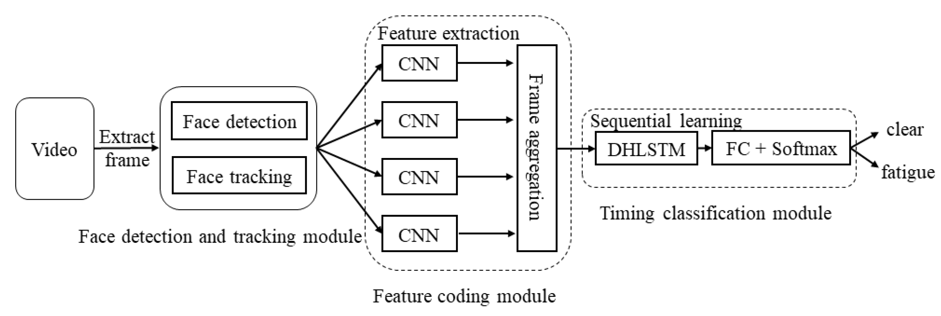
The method proposed in this paper mainly consists of three modules, including a face detection and tracking module, a feature coding module and a temporal classification module.
Figure 1 shows the overall flow of the method.
Extracting the frames from the video. The method needs to locate the key facial points and extract the ROI of the eye and the mouth one by one through the face detection and tracking module.
Extracting features of the ROI sequence through a CNN and encoding the feature information to construct feature vectors through a frame aggregation method.
Inputting the feature vector sequence into a double-hidden long short-term memory neural network (DHLSTM) to learn time sequence features and then make a global decision on the video sequence to predict whether the driver is fatigued.
2.1. Face Detection and Tracking
There are some challenges for face detection in open-pit trucks. Firstly, the proportion of the face in the image is small, and the complex background interferes greatly with face detection. Secondly, due to irregular installation of cameras on different trucks and rotation of the driver’s head, the orientation of the face in the video sequence varies widely. When dealing with such a challenging task, the general face detection algorithms are not able to take into account the speed and accuracy at the same time.
Libfacedetection is an open-source library for image face detection which adopts a lightweight face detection algorithm based on the SSD architecture proposed by Yu Shiqi. The algorithm is robust and suitable for face detection in complex backgrounds. Moreover, it can detect multiangle faces fast and accurately.
Although face detection speed in a single frame is very fast, it is still very time-consuming to detect the face in an image sequence frame by frame without considering the connection between the previous and subsequent frames. In an image sequence, the driver’s actions are continuous in the time domain and change relatively slowly in the space domain. According to these features, this paper integrates a tracking method to optimize the face detection module. The method tracks the face regions of adjacent frames by utilizing the spatiotemporal relationship between the adjacent frames.
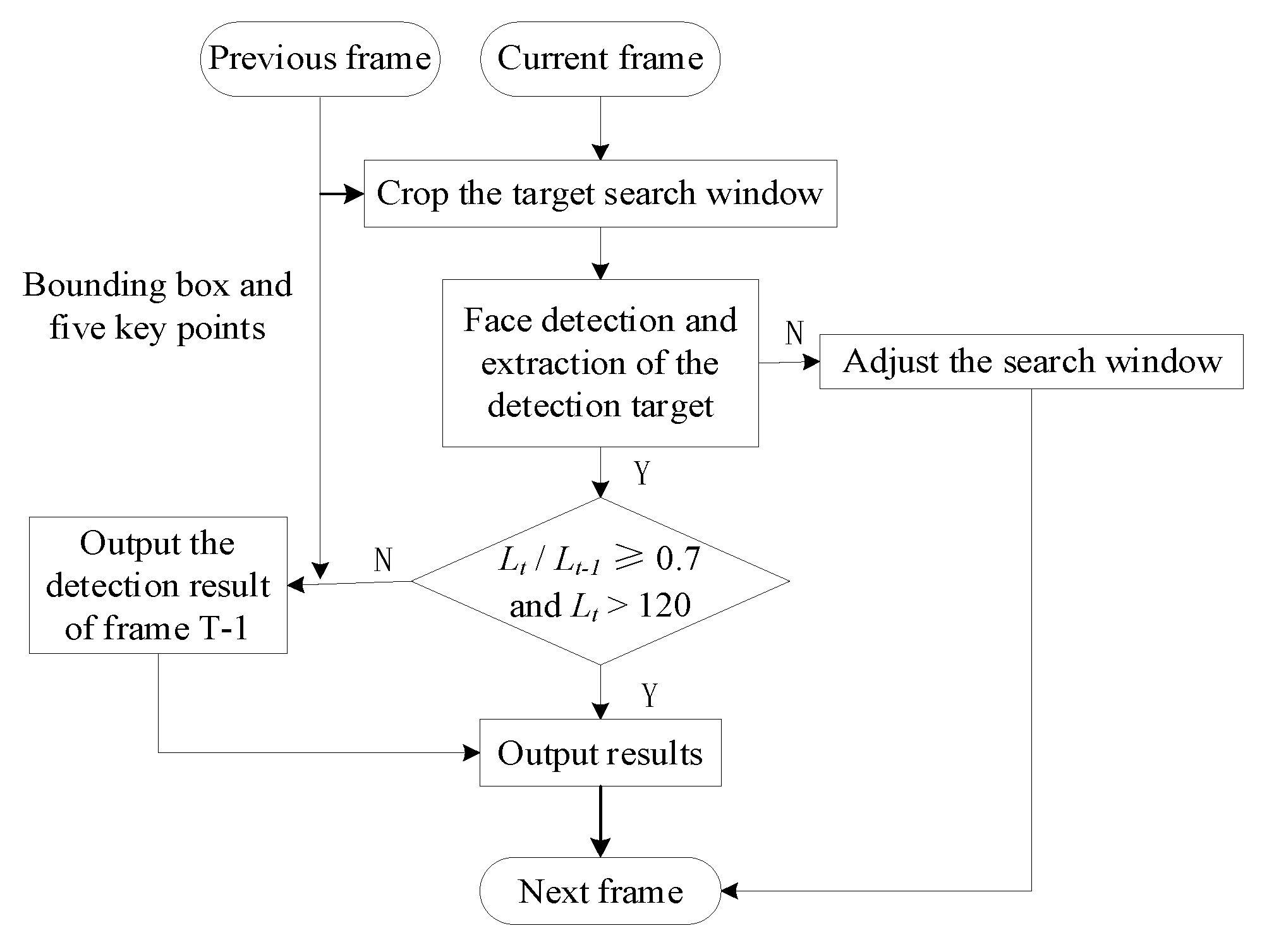
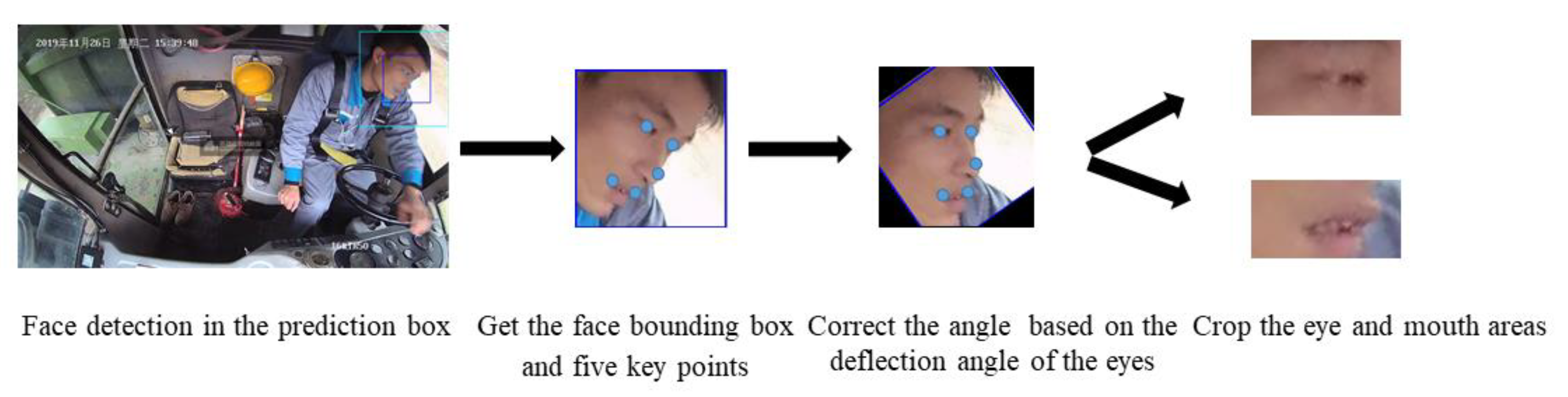
Figure 2 shows the overall workflow of the algorithm.
The method needs to obtain the previous frame detection result before the current frame is processed. The centerpoint of the bounding box belonging to the previous frame is taken as the prediction centerpoint of the face region in the current frame. According to this centerpoint, this method doubles the bounding box of the previous frame to obtain a new bounding box and uses the new bounding box to crop the current frame. The cropped image is input into the face detection model. In the dataset, the size of the face in the picture has a lower limit, and the ratio of the side length of the next frame to the side length of the previous frame should not be lower than a certain threshold. Thus, by judging the side length of the bounding box and the size of the bounding box in two adjacent frames, the prediction bounding box of the current frame is adjusted accordingly. The method limits the detection region of the next frame through the connection between the adjacent frames, which can effectively eliminate background interference and greatly reduce the computational cost.
2.2. LRCN for Fatigue State Classification
An LRCN is a network constructed by combining a CNN and an LSTM, which has the ability of spatial feature extraction and long-term sequence learning. This paper proposes a network structure by combining Resnet and a DHLSTM to deeply explore the spatiotemporal features of driver fatigue.
Residual network is the most widely used CNN network at present. It adds residual units based on Vgg19 [
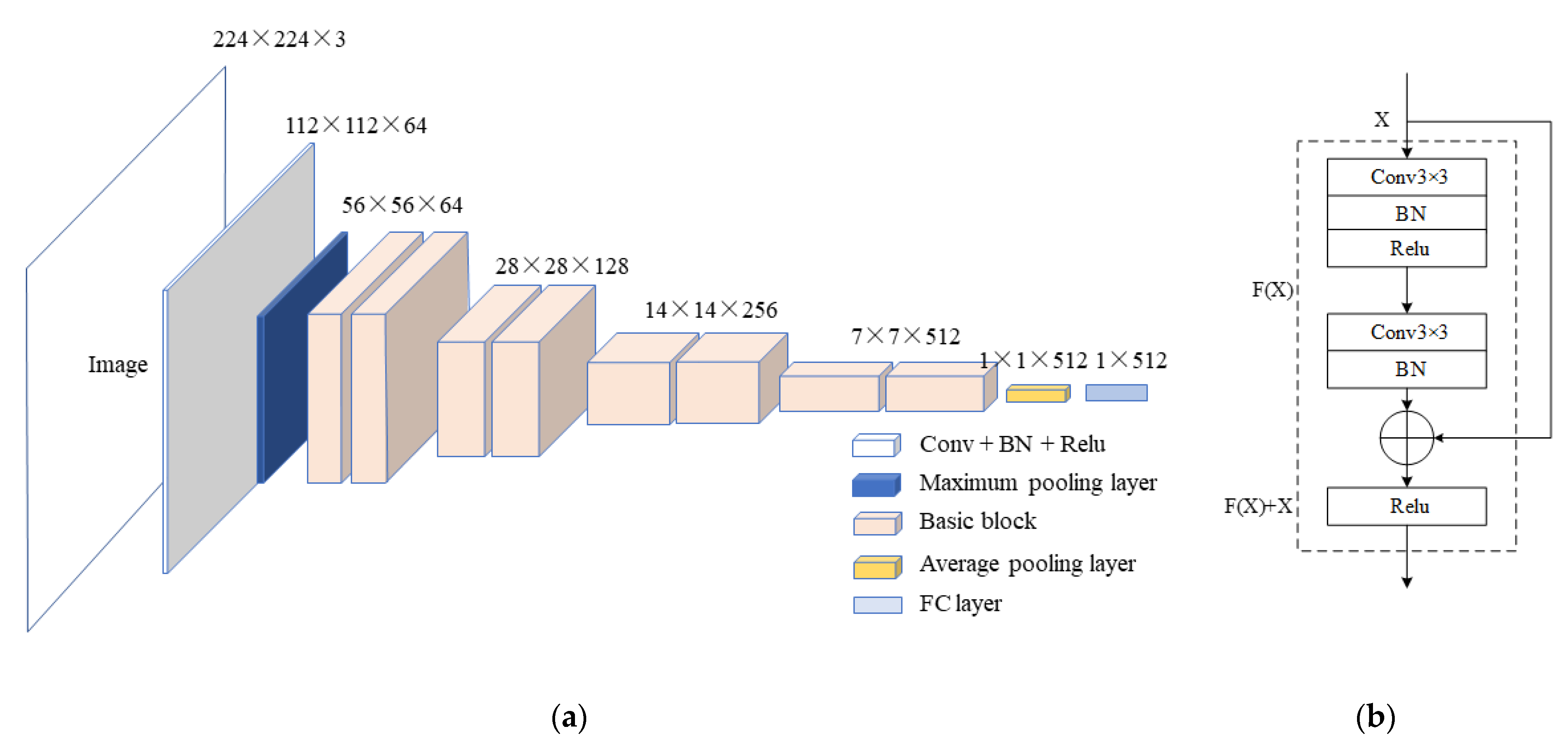
26] and makes a skip connection between every two convolutional layers to form residual learning, which makes Resnet a great success in solving the problems of gradient disappearance and gradient explosion in deep networks. It maintains the advantage of deep networks in image feature excavation. Taking account of the complexity of features and the size of the model, Resnet18 is used as the feature extraction network to process video frames. The Resnet18 structure consists of 18 network layers, including the convolution layer with a convolution kernel of 7 × 7, the maximum pooling layer, eight basic blocks, the average pooling layer and the full connection layer.
Figure 3a shows the structure. Each basic block is composed of two convolution layers with a convolution kernel of 3 × 3. Each convolution is configured with a batch normal (BN) layer and a Relu layer.
Figure 3b shows a basic block.
The learning principle of residual units can be defined as follows.
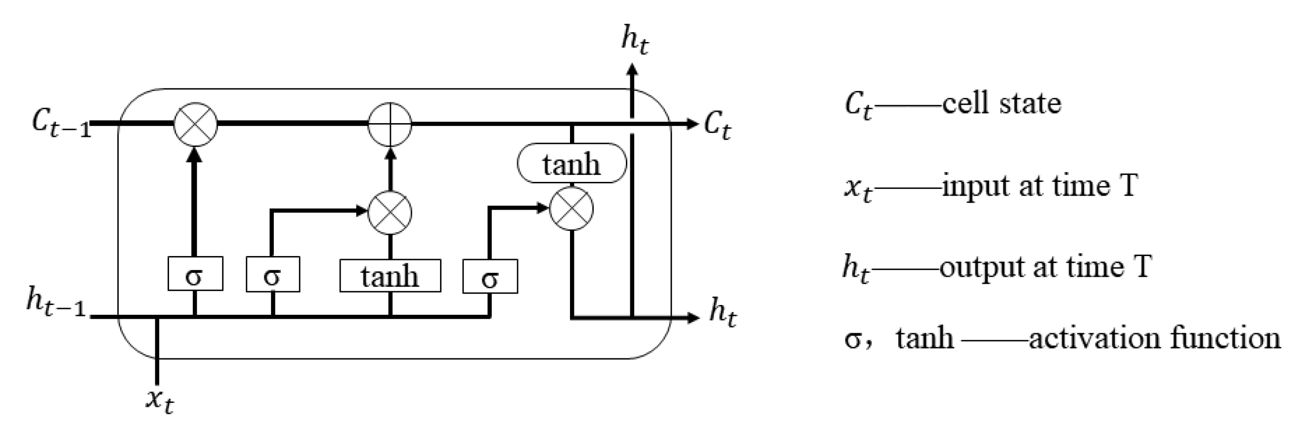
A long short-term memory (LSTM) network is an improved RNN. Unlike convolutional networks which are better for processing single images, LSTMs are good at dealing with long-time dependent problems. An LSTM is composed of multiple units. Each unit contains three essential parts, which are the input gate, the forget gate and the output gate. Through the gates, an LSTM can integrate and filter the input information of multi-moments to achieve long-term memory.
Figure 4 shows the unit structure.
The gates are defined as follows.
Output gate:
where
,
and
represent the attenuation coefficient of learning different memories, respectively,
,
represent the memory learned before time T and the memory learned at the current moment, respectively,
represents the memory state at time T and
represents the network output at time T.
A DHLSTM is a variant of an LSTM. It adds a layer of hidden cells to the original LSTM. Two hidden layers are stacked for calculation, which is beneficial for the network to excavate more information between the sequences [
29]. In addition, an LSTM has variants such as gated recurrent (GRU) and bidirectional long short-term memory (Bi-LSTM) networks.
2.3. Feature Coding Strategy
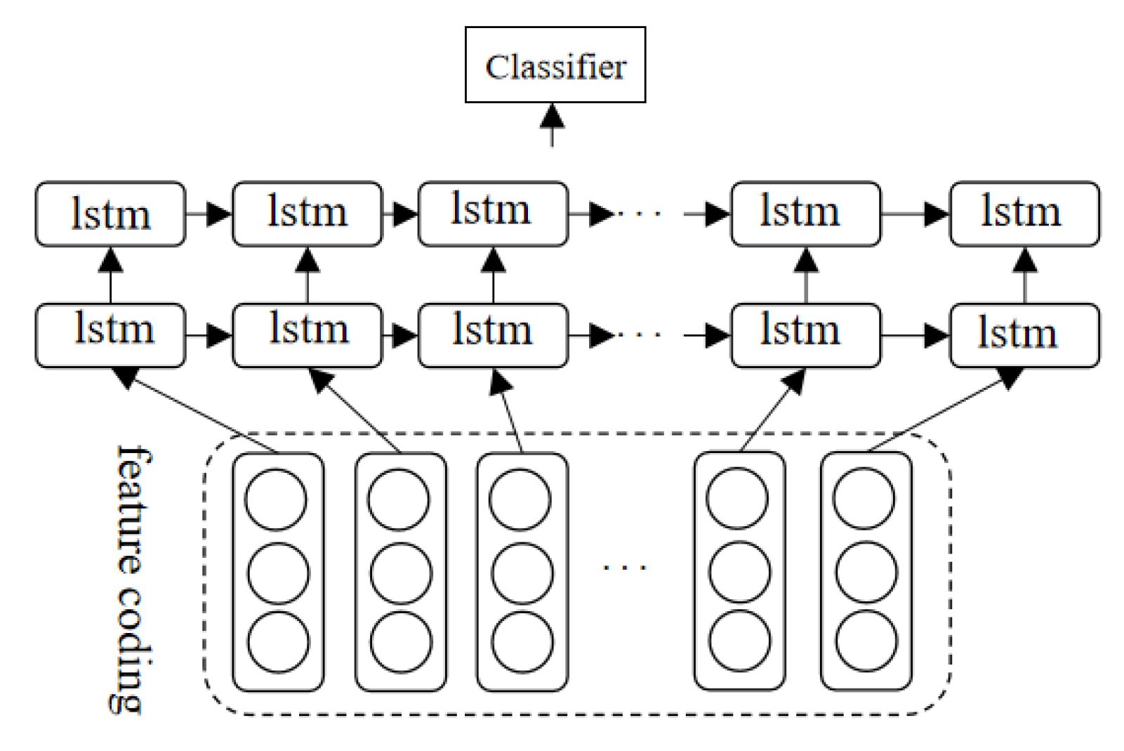
As shown in
Figure 5, the hidden states of all moments in a DHLSTM are collected as features of the input sequence and then input into the classifier for time sequence classification [
30]. The hidden states at each moment represent the learning situation of the input data at the current moment. Before learning these features, the data cannot be directly input into a DHLSTM in the form of image sequences, and they need to be converted to a vector sequence when a DHLSTM processes the time sequence data of the image type. This process is called coding.
The coding of image sequences involves frame aggregation and uses a feature vector to represent the image sequence over a period of time [
31]. Different coding strategies of the image sequence obtain different feature representations, which affect the classification results of the DHLSTM model and the performance of the whole network. Thus, this paper proposes three coding strategies based on feature-level and decision-level frame aggregation.
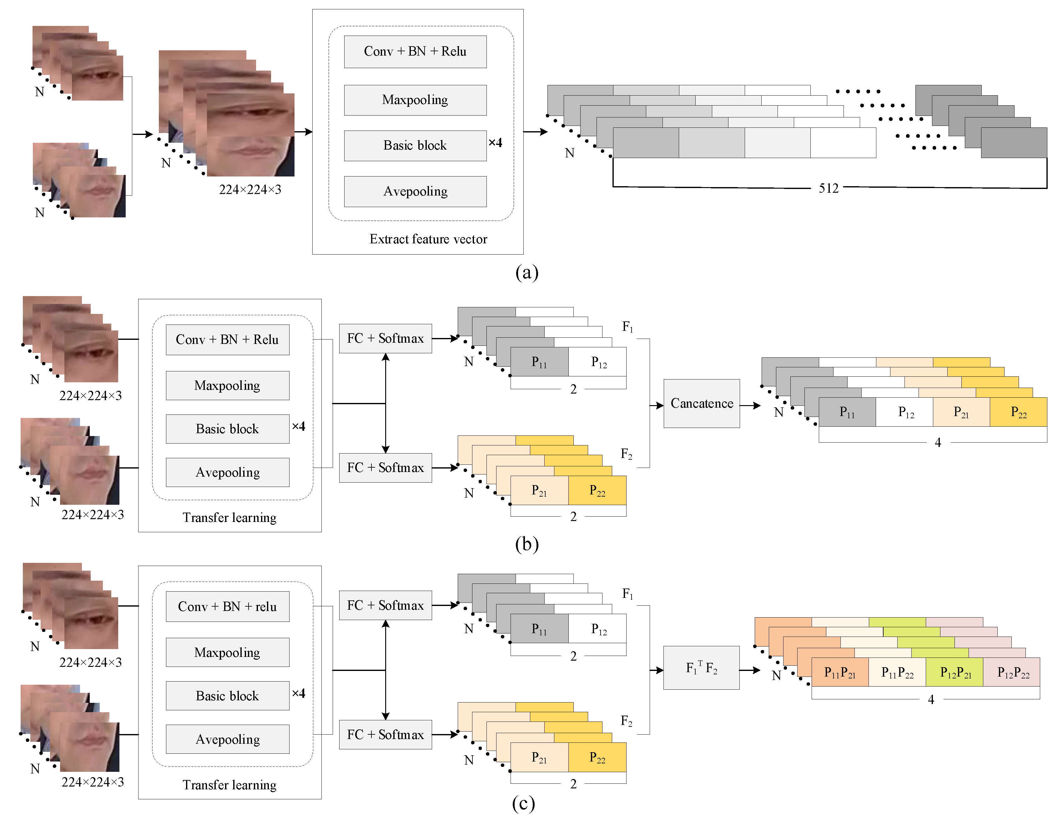
Figure 6 shows the structure of each strategy.
Figure 6a shows the structure of feature-level frame aggregation. The coding strategy performs convolution processing on each frame to obtain a feature map containing information on edges and shapes. The feature map of each frame is converted into a 512-dimensional feature vector and stacked across time. This coding strategy can retain the representation of most original image information so that the LSTM can pay attention to more details when learning time sequence features. The initial parameters of the model are obtained through transfer learning. The parameters of the convolutional layers in the pretraining model [
24] are frozen as the initial parameters used to extract the spatial features of the eye–mouth stitching images. Then, the convolution layer and the top layer are jointly trained to update the network weight.
Decision-level frame aggregation is a process that integrates the decision information of multiple feature classifiers. As shown in
Figure 6b,c, this paper constructs a dual-convolution network to classify eye features and mouth features, respectively. The strategy obtains two classification probabilities through the two classifiers. Then, all local information is encoded through different feature fusions. In the process of time sequence learning, the classification results of multiple features can change from local classification decisions to a global classification decision. There are two strategies based on different feature fusions.
Figure 6b shows decision-level frame aggregation based on vector stitching. After obtaining two two-dimensional vectors from the eye classifier and the mouth classifier, the strategy fuses the features of the two vectors by stitching the vectors and stacks them across time.
Figure 6c shows another strategy which adopts the method of the feature vector dot product for feature fusion and coding. Both training methods are the same. Firstly, the eye and mouth classifiers are trained through the two self-built datasets of the eye and the mouth. To obtain classification results of the driver’s eye status (open or closed) and mouth status (open or closed), the Resnet18 pretrained model is used to train the eye and mouth classification models. Then, the output results of the classifiers are aggregated and input into the DHLSTM for global training.
4. Discussion
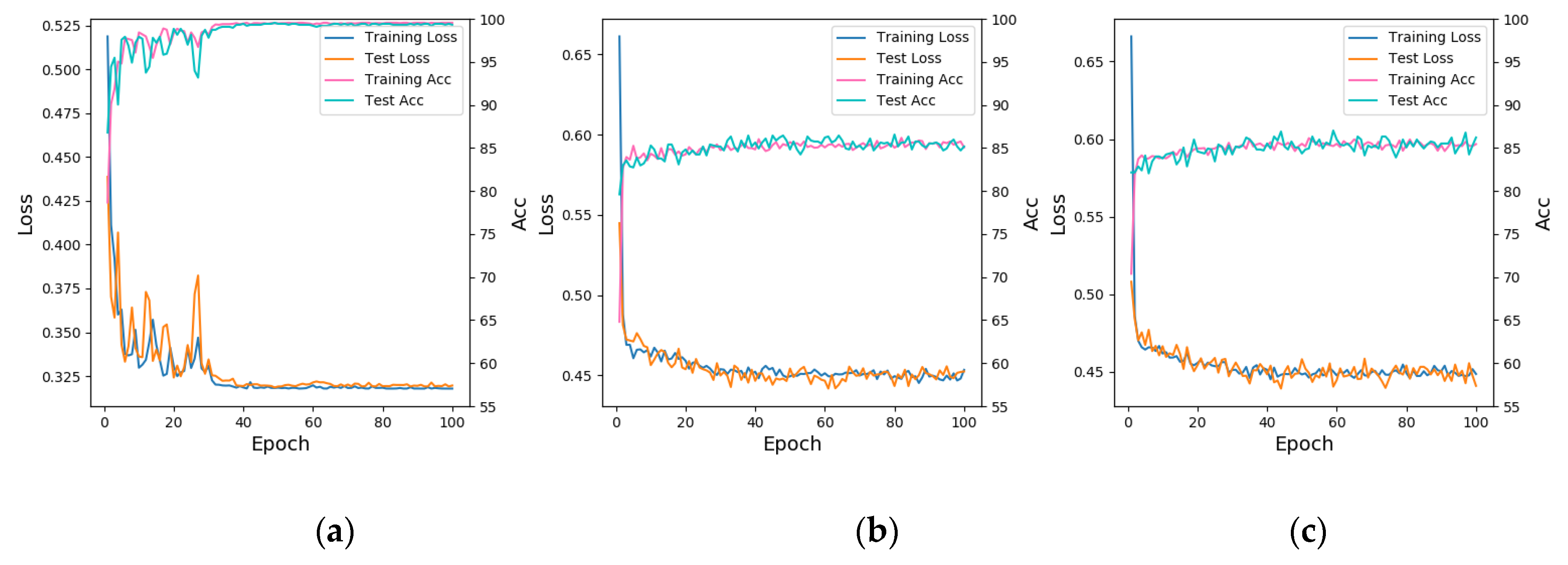
4.1. Training Process
Loss and accuracy of three schemes above performed well in training. Among them, model 2 and 3 were faster than model 1 in convergence speed when training. Meanwhile, the loss and accuracy of models 2 and 3 preformed more stably at the initial training stage, but model 1 was more accurate in the training set and the test set.
4.2. Accuracy
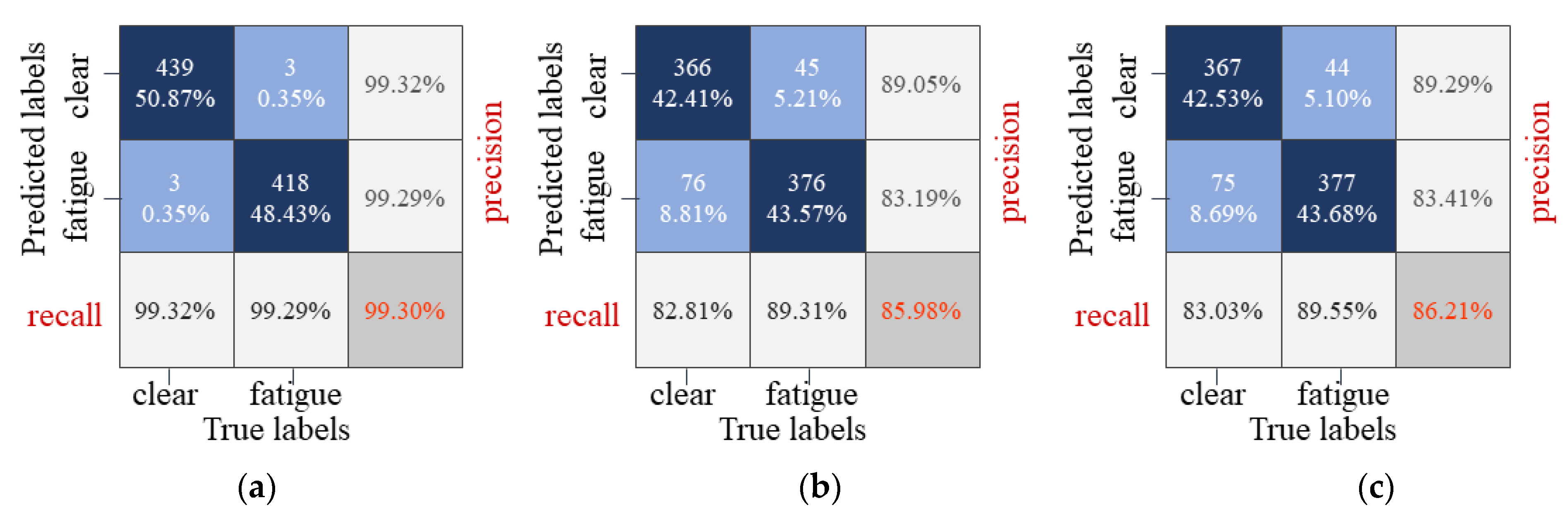
It is worth noting that it was impossible to obtain the real label of the driving status in our task. Based on the general facts, this paper makes a qualitative judgment to label samples by observing the driver state, such as slow blinking, continuous eye closing, yawning, etc. The time sequence classification model based on feature-level frame aggregation performed better than the time sequence classification model based on decision-level frame aggregation in terms of accuracy and recall rate. It may be that frame aggregation based on the feature level can obtain more time sequence information in this task, which helps the DHLSTM network to deeply excavate the time sequence features of the target object. However, the information obtained by means of decision-level frame aggregation is relatively singular; the accuracy of the global classification decision is limited by the accuracy of local classifiers. Therefore, it is difficult to improve the accuracy of models 2 and 3 to a higher level. Model 1 was better suited to driver fatigue detection in this task.
4.3. Time Sequence Classification Models
Different time sequence learning networks have different performance in excavating the time domain information, which has a great impact on the classification accuracy. In order to find a model to better excavate time sequence features, this paper compares multiple networks. Due to the small sample size of the self-built dataset, there were certain limitations. The public dataset was used to test the performance of different time sequence learning models based on feature-level frame aggregation. The results are shown in
Table 3.
According to
Table 3, the accuracy of the time sequence learning model based on the several LSTM variants in the training set above was over 90%. Among them, the model composed of GRU and Resnet had the best fitting effect on the training set, and the accuracy was 95.5266%. The model composed of a DHLSTM and Resnet performed best on the test set with the accuracy of 92.6180%.
The accuracy difference of the training set and the test set can reflect the generalization ability of the model. The model composed of an LSTM and Resnet and the model composed of a Bi-LSTM and Resnet showed a larger accuracy difference than the other models, and the accuracy of the two kinds of models was 10.3% and 9.8%, respectively, which represents a trend of overfitting. The time sequence learning model with a DHLSTM network showed the smallest accuracy difference and the best fitting effect. Therefore, it can be seen that a DHLSTM performs better in terms of exploring time sequence features.
4.4. Model Speed
A tracking method was added to optimize face detection, which was helpful to improve detection accuracy and reduce detection time. The detection speed and the false detection rate are shown in
Table 4, and the detection time expenditure of each module after optimization is shown in
Table 5.
Table 4 shows the time expenditure and accuracy results of face detection with the tracking method and without the tracking method. When detecting the same image sequence, the average detection time without the tracking method was 0.2886 s per frame and the average detection time with the tracking method was 0.075 s per frame. The time difference is obvious. In comparison with the face detection module without the tracking method, the face detection module with the tracking method reduced the detection time expenditure by 74%, and the false face detection rate decreased from 16.7% to 3.33%.
Table 5 shows the time expenditure of each module for a sample. The total inference time for detecting a 30-frame image sequence was about 2.85 s. Among them, the detection time of the face detection and tracking module was 2.25 s per 30 frames. The time of the coding module based on feature-level frame aggregation was 0.517 s per 30 frames. The time of the time sequence classification module was 0.076 s per 30 frames.
It can be seen from the time analysis that the detection time was mainly concentrated in the face detection module. It takes a long time because a scene on the paper is more complex than other scenes, such as the face angle relative to the camera, light and other environmental interference factors. In order to speed up, this paper proposes a tracking method, which shows a significant reduction in time expenditure. Although the optimized face detection module had a great improvement in detection speed, the real-time performance still needs further research.
5. Conclusions
This paper proposed a video-based driver fatigue detection method for open-pit truck drivers. The method can overcome the interference caused by a complex environment. The innovation of this paper is to combine Resnet with a DHLSTM to build a spatiotemporal network model suitable for this task. Resnet extracts the spatial features of each frame, and then the extracted spatial features are aggregated and input into a DHLSTM for temporal feature learning and classification. Meanwhile, the paper adds a tracking method to the face detection module to reduce the detection time expenditure. The face region is tracked by utilizing the spatiotemporal relationship between the adjacent frames. The experimental results show that the method can effectively detect the driver fatigue behavior in image sequences. In comparison with the face detection module without the tracking method, the time expenditure of the proposed method is reduced by 74% at the face detection stage, which is better suited to face detection in complex environments. Moreover, the LRCNs composed of Resent and a DHLSTM perform better in features excavation and generalization than LSTM, GRU and Bi-LSTM and can achieve more accurate classification results. The paper determined driver fatigue on the basis of video sequences of 30 frames. The results show that the method can meet the requirements of practical applications to a certain extent in terms of accuracy and speed. When combined with other necessary hardware equipment, this method can be deployed for application in practice.
The method proposed in this paper still has certain limitations. The method does not classify the level of fatigue. In the future, this method will be improved to classify the level of driver fatigue. For occlusion situations, such as mouth covering, eye rubbing, etc., this paper does not make an effective response. Future research will pay more attention to unobstructed parts when the face is occluded to detect driver fatigue. The optimized face detection stage has a great reduction in detection time expenditure, but the real-time performance still needs further improvement.


