Comparison of Molecular Geometry Optimization Methods Based on Molecular Descriptors

Abstract

Various methods (Hartree–Fock methods, semi-empirical methods, Density Functional Theory, Molecular Mechanics) used to optimize a molecule structure feature the same basic approach but differ in the mathematical approximations used. The geometry optimization procedure calculates the energy at an initial geometry of a molecule and then proceeds to search a new geometry with a lower energy. Using the 3D structures collected from the PubChem database, 20 amino acid geometry optimization calculations were performed with several methods. The purpose of the study was to analyze these methods (39) to find the relationship between them and to determine which to use under different circumstances. Cluster analysis and principal component analysis were performed to evaluate the similarities between the different methods. The results after the analysis can classified into three main groups and can be selected accordingly to solve different types of problems.

1. Introduction

A basis set is essentially a finite number of atomic-like functions, over which the molecular orbital is formed via linear combination of atomic orbitals (LCAO). There are multiple choices for the basis set, such as Slater type orbitals [1] (STOs) or Gaussian-type orbitals [2] (GTOs). The wave functions are also called “stationary states” or “energy eigenstates”; in chemistry they are called “atomic orbitals” or “molecular orbitals”. Consequently, they are important in molecular modeling [3,4].

Stationary states be described by the time-independent Schrödinger equation:

$$\mathit{H}\mathit{\psi }=\mathit{E}\mathit{\psi },$$

(1)

where ψ is the state vector of the quantum system, E is the energy, and H is the Hamiltonian operator.

In the time-independent Schrödinger equation, the operation may produce specific values for the energy called energy eigenvalues. In addition to its role in determining system energies, the Hamiltonian operator generates the time evolution of the wavefunction in the form:

$$\mathit{H}\mathit{\psi }=\mathit{j}\hslash \frac{\mathit{\partial }}{\mathit{\partial }\mathit{t}},$$

(2)

where the j constant is the imaginary unit, $\hslash$ is the reduced Planck constant, and t is time.

The Schrödinger equation provides a method for calculating the wave function of a system and its dynamic change over time. The equation is a wave equation in terms of the wave function which predicts analytically and precisely the probability of events or outcome. The spatial part needs to be solved for in time-independent problems, because the time-ependent phase factor is always the same.

The Schrödinger Equation (1) for molecular systems can only be solved approximately [5]. The energy operator can be replaced by the energy eigenvalue E, so the time-independent Schrödinger equation is an eigenvalue equation for the Hamiltonian operator. Approximation methods can be classified into ab initio or semi-empirical categories.

An unknown one-electron function, such as an orbital ψ_i can be expanded in a set of known functions χ_k (k = 1, 2, …, M), the basis set:

$${\mathit{\psi }}_{\mathit{i}}={\displaystyle \mathbf{\sum }}_{\mathit{k}=\mathbf{1}}^{\mathit{M}}{\mathit{c}}_{\mathit{k}\mathit{i}}{\mathit{\chi }}_{\mathit{k}}.$$

(3)

In Hartree–Fock (HF) and Kohn–Sham density function theory (DFT), the coefficients c_ki are determined by minimizing the total energy, which by traditional methods lead to a matrix eigenvalue problem that is solved iteratively to provide a self-consistent field (SCF) solution.

The foundations of the orbital theory were laid by Hartree, Fock, and Slater. If the 2n electrons in a molecule are assigned to a set of n molecular orbitals ψ_i (i = 1, …, n), the corresponding many electron wavefunction is:

$$\psi ={\left(2n!\right)}^{-1/2}\det \left[\left(\psi \_1\alpha \right)\left(\psi \_1\beta \right)\left(\psi \_2\alpha \right)\dots \right].$$

(4)

The ψ_i are orthonormal and α and β are spin functions.

Slater-Type Orbitals (STOs) and Gaussian-Type Orbitals (GTOs) are used to describe AOs (atomic orbitals). STOs describe the shape of AOs more accurately than GTOs, but GTOs feature an advantage: they are much easier to compute. In fact, calculating multiple GTOs and combining them to describe an orbital is faster than calculating an STO. This is why combinations of GTOs are usually used to describe STOs, which, in turn, describe AOs.

The simplest and standard basis set in the Gaussian Program is Slater-Type- Orbitals simulated by three Gaussian functions each (STO-3G). Generally, if n < 3 the calculations produce poor results, in consequence, STO-3G is called the minimal basis set. We use minimal basis sets for qualitative results, very large molecules, or quantitative results for very small molecules (atoms) [6]. STOs represent the exact solutions for hydrogen-like atoms and provide a better representation than Gaussian functions for multielectron systems on a function-to-function comparison.

The most commonly used bases set for geometry optimization is 3-21G [7,8,9]. This method uses three Gaussians for the core orbitals and a two/one split for the valence functions. Usually, d orbitals for all heavy (non-hydrogen) atoms are added to improve a basis set. The polarization basis sets are those that include the d orbitals; they are indicated by the symbol “*”. A further development is the 6-31G** basis, in which a set of p orbitals is added to each hydrogen in the 6-31G* basis set [10].

A number of methods are used to optimize the geometry of molecules: empirical force field methods (molecular mechanics, a cheaper method in terms of computational speed, able to provide exceptional structural parameters), semi-empirical methods (to solve the Schrödinger equation, with certain approximations and description of the electron properties of atoms and molecules), and ab initio methods (e.g., Hartree–Fock, Post-Hartree-Fock, and Density Functional Theory) [6].

John A. People [11] pioneered the development of ab initio methods using Slater type bases sets or Gaussian orbitals to model the wave function. He defined models, selecting a combination of methods and bases sets, and compared the experimental results of the analysis. With his team, he established an extended basis of contracted Gaussian functions that considers the same properties but is still simple enough to be widely applied to organic molecules [10]. Gaussian-type atomic orbitals have been used broadly to calculate atomic and molecular wavefunctions. They were involved in the growth of one of the most common computational chemistry packages, the Gaussian programs.

For ab initio methods, the first step is a single-determinant SCF (self-consistent field) calculation. Ab initio quantum chemistry methods present the challenge of solving the electronic Schrödinger equation based on the positions of the nuclei and the number of electrons to provide valuable data.

Their quality depends on the basis set used. The Hartree and Hartree–Fock methods can be regarded as reference methods for many calculations in complex systems. The first solutions to be obtained are used in the next iteration. Hartree-Fock equations must be solved by an iterative procedure and offer the second set of solutions. This approach, SCF, continues as long as the energies of all the electrons remain unaffected. Almost all ab initio calculations use GTO basis sets.

Pure density functional theory (DFT) [12,13] methods are characterized by pairing an exchange functional with a correlation functional. Most current DFT studies use BP86, B3LYP, or BPW91 functionals.

The combination of the method and the basis set determines the chemistry model as Gaussian, specifying a level of theory. HF methods are considered the default if no other keywords are mentioned. Most methods also require a basis set; if no basis set keyword is specified, then STO-3G is used automatically. Some examples of basis sets are: STO-3G, 3-21G, 6-21G, and 6-31G. Single first-polarization functions can also be requested by using the usual * or ** notation. 6-31G* (or 6-31G(d)) is 6-31G with additional d polarization functions on non-hydrogen atoms; 6-31G** (or 6-31G(d, p)) is 6-31G* plus p polarization functions for hydrogen [5]. The + and ++ diffuse functions are accessible with some basis sets. 6-31+G is 6-31G plus diffuse s and p functions for non-hydrogen atoms; 6-31++G also features diffuse functions for hydrogen. Thom Dunning introduced optimized basis sets with correlated wavefunctions: cc (correlations-consistent basis) or pV (polarized valence basis) [14]. The prefix aug (augmented) can be used to add diffuse functions. Which a basis set is used, it is related to the purpose of the calculation and the molecules to be studied. Even a large basis set is not always a guarantee of agreement with the experimental data [13,15].

Different approaches [16,17,18] to the comparison of basis sets agree that, even if they are similar, basis sets cannot be generalized. Some recommendations we found in the articles studied and by consulting Gaussian tutorials are:

A large basis set is not always the best (ex: cc-pVQZ is overkill for Hartree-Fock).

The minimal basis set (STO-3G) allows the analysis of the largest molecules while having the lowest resolution/quality for quantum level. In general, cc-pVDZ is equivalent to or worse than 6-31G (d, p).

cc-pVTZ is better than 6-311G(d,p) or similar.

The convergence of ab initio methods is time-consuming.

The following bases sets are approximately equivalent:

• 6-31G → cc-pVDZ
• 6-311G → aug-cc-pVDZ
• 6-31+G(d) → cc-pVTZ
• 6-311+G(d) → aug-cc-pVTZ
• 6-31++G(d,p) → cc-pVQZ
• 6-311++G(d,p) → aug-cc-pVQZ

Due to the many basis sets and optimization methods, it is very difficult to find the optimal approach for scientific calculations. The choice of basis set for chemical calculations can have a major impact on the quality of the results, particularly for correlated ab initio methods [19]. The choice can be made based on the knowledge related to the design, development, and optimization of the latest developments in the field. For example, applications of basis sets are in the simulation and optimization of ultrasonic non-destructive tests, which are highly important in structural materials such as fiber composites, but also in columnar grained stainless steels [20]. Another approach could be functional cluster analysis (FCA) for multidimensional functional datasets, using orthonormalized Gaussian basis functions, which can be applied for example, to protein structures [21].

The purpose of this study was to analyze 39 optimization methods to find the relationship between them and determine which to use under different circumstances. Cluster analysis, Statistical analysis (ANOVA), and principal component analysis (PCA) were performed to evaluate the similarities between the different methods.

2. Materials and Methods

The 20 amino acid structures (3D) shown in

Table 1. Amino acids used as input data to our algorithm.

Amino Acids (AA)
Arginine	Lysine	Methionine	Leucine
Asparagine	Serine	Alanine	Phenylalanine
Aspartate	Threonine	Valine	Proline
Glutamate	Cysteine	Glycine	Tryptophan
Glutamine	Histidine	Isoleucine	Tyrosine

were collected from the PubChem compound database [22].

These 20 amino acids feature different forms, isomers, enantiomers, and conformers. In biological systems, amino acids feature the same chirality; most are levorotatory (L) and not dextrorotatory (D). Using the L conformer of these compounds, geometry optimizations were performed on the structures (

Table 2. Geometry optimization methods used in the calculations.

Gaussian Optimization Methods
Semi-Empirical Methods (Default Spin)	1. Parameterized Model 6 PM6 (opt-pm6) 2. Austin Model 1 AM1 (opt-am1) 3. Parameterized Model 3 PM3 (opt-pm3) 4. Parameterized Model 3 (Molecular Mechanics correction) PM3MM (opt-pm3mm) 5. Pairwise Distance Directed Gaussian function PDDG (opt-pddg) 6. Complete Neglect of Differential Overlap CNDO (opt-cndo) 7. Intermediate Neglect of Differential Overlap INDO (opt-indo)
Density Functional Theory (Default Spin)	Becke(three-parameter)–Lee–Yang–Parr (functional) B3LYP 8. opt-b3lyp-sto-3g; 9. opt-b3lyp-3-21g; 10. opt-b3lyp-6-31g; 11. opt-b3lyp-6-311g; 12. opt-b3lyp-cc-pvdz;) Local Spin Density Approximation LSDA 13. opt-lsda-3-21g; 14. opt-lsda-sto-3g; 15. opt-lsda-cc-pvdz; 16. opt-lsda-6-311g; 17. opt-lsda-6-31g;) 18. Perdew–Burke-Ernzerhof (functional) PBEPBE opt-pbepbe-sto-3g BVP86 19. opt-bvp86-sto-3g; 20. opt-bvp86-3-21g; 21. Opt-bvp86-6-31g; 22. opt-bvp86-6-311g;) B3PW91 23. opt-b3pw91-sto-3g; 24. opt-b3pw91-6-31g; 25. opt-b3pw91-6-311g;)
Møller–Plesset Perturbation Theory	MP2 26. opt-mp2-sto-3g; 27. opt-mp2-3-21g; 28. opt-mp2-6-31g; 29. opt-mp2-6-311g; 30. opt-mp2-cc-pvdz;)
Coupled-Cluster Theory	31. Coupled Cluster single-double CCSD (opt-ccsd-sto-3g)
Molecular Mechanics (Default Spin)	32. Universal Force Field UFF (opt-uff) 33. Dreiding (opt-dreiding)
Hartree–Fock (Default Spin)	34.STO-3G(opt-hf-sto-3g) 35.3-21G(opt-hf-3-21g) 36.3-21G*(opt-hf-3-21g*) 37.6-31G(opt-hf-6-31g) 38.6-311G(opt-hf-6-311g) 39.CC-pvdz(opt-hf-cc-pvdz)

). The most frequent procedure to establish the basis functions describing the occupied atomic orbitals by HF/DFT optimization followed by addressing the issue of polarization functions subsequently. Whatever optimization method is used, it defines a local minimum, and it is possible that optimization starting from different initial exponents will lead to different outcomes.

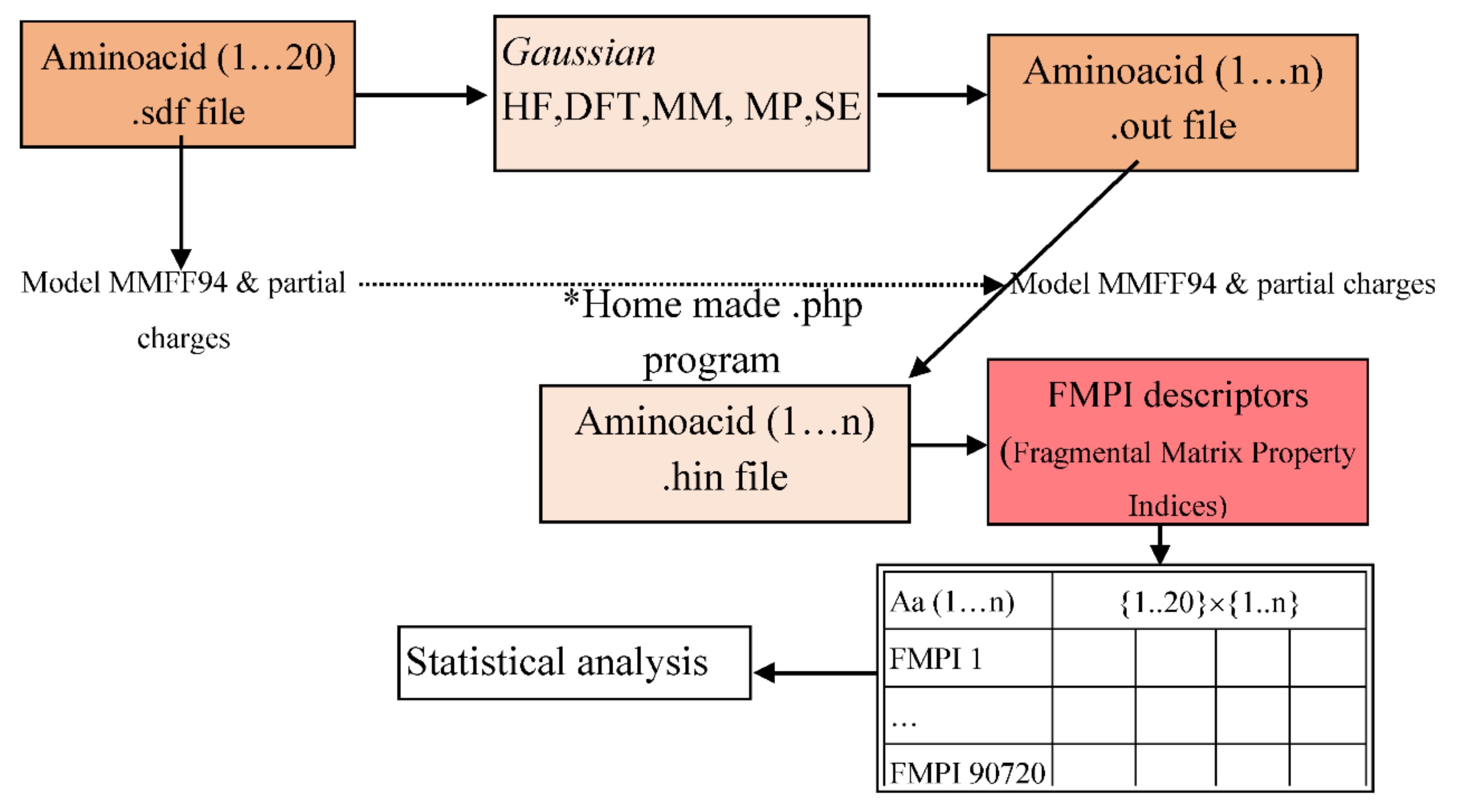
The workflow is represented in the next figure (Figure 1). After the Gaussian program made the calculations based on the 39 methods selected, a family of molecular descriptors (FMPI- Fragmental Matrix Property Indices) [23] was also calculated to evaluate the degree of similarity between the methods. The results were submitted to cluster, PCA, and other statistical analyses.

We collected the structures (3D) of the 20 essential amino acids (L conformers) from PubChem databases (.sdf files) and analysed them with the Gaussian program, taking into consideration the following steps, also shown in Figure 1:

• Enter the PubChem .sdf files to the Gaussian program.
• Save the file in .gjf file format (the input file format for the program).
• Analyse the amino acids using the following t command: Calculate → Gaussian Calculation Setup → Job type (Optimization).
• From the Calculation Setup menu select the Gaussian Geometry Optimization Methods one after another and run the calculations.
• Save for every calculation the .out file (the output file format for the program).

With a homemade *php program we generated .hin files from the .sdf files and generated the molecular descriptors (FMPI). FMPI molecular descriptors are the improved version of SMPI (Szeged Matrix Property Indices) [24,25] descriptors. With SMPI, distance matrix are calculated, and then for each pair of (distinct) atoms the atoms closer to the first than to the second atom of the pair are collected into a matrix [15]. The improvement made to SMPI is the extension of the principle applied in Szeged fragments to the other two matrices collecting fragments from molecules for pairs of atoms.

Therefore, the gene sequence of FMPI was increased from SMPI with one gene and the number of descriptors was multiplied by three (arriving at 4536) [23]. After we obtained 4536 descriptors for every amino acid, we used the Statistica program to perform the clustering and PCA analysis.

3. Results and Discussion

After applying the algorithm described in the Methodology section, a principal component analysis (PCA) and a clustering analysis were performed. The next figure (Figure 2) shows the first and second component as the result of the PCA analysis.

Each principal component is a linear combination of the variables from the whole data set. A total of 90,720 descriptors for each component and each method were analysed, or a total of 3.538.080 descriptors.

The result of the PCA analysis indicated that the principal components (Figure 2) explained our large amount of data at 99.8851%, which reflected the variance of the data.

The first component accounted for a maximum amount of total variance (71.25%) in the data analysed. The second component accounted for the maximum variance that was not explained by the first component (14.9%). The third component also accounted for the maximum variance (6.51%) after the first two.

The R²X describes the predictive accuracy and takes values between 0 and 1. The more significant a principal component, the larger its R²X. The explained variance (R²X_adj) is simply the explained variation (R²X) adjusted for the degrees of freedom.

The quality assessment, goodness-of-prediction (Q²) statistic is typically reported as a result of cross-validation and provides a qualitative measure of consistency between the predicted and original data. As we add more variables to the PCA analysis, the value of Q² increases. Large values of Q² indicates a relevant and significant analysis.

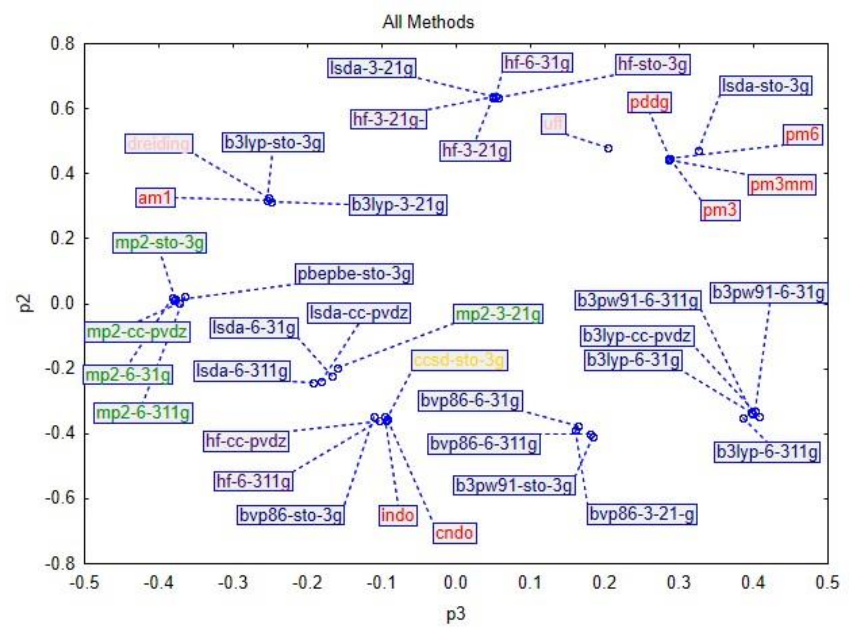
In the next figure (Figure 3), a score loading plot, the distribution of component 1 versus component 2 is represented. The plot indicates that the similar methods are indeed roughly grouped together. Furthermore, the loadings define the orientation of the principal components in space. The loading vectors are p1 and p2. In our case, the first three components explained most of the data. In the next figure, a score loading plot, the distribution of component 3 versus component 2 is represented (Figure 4).

The classification of the methods into four categories (Semi-Empirical, Density Functional Theory, Molecular Mechanics Møller–Plesset Perturbation Theory, Coupled-Cluster Theory and Hartree–Fock) in the Section 2 is not entirely valid if we take into consideration the similarity between them. The degree of similarity between the methods grouped the data into the main categories presented above, but also into different and mixed groups. The PCA and cluster analyses produced comparable results.

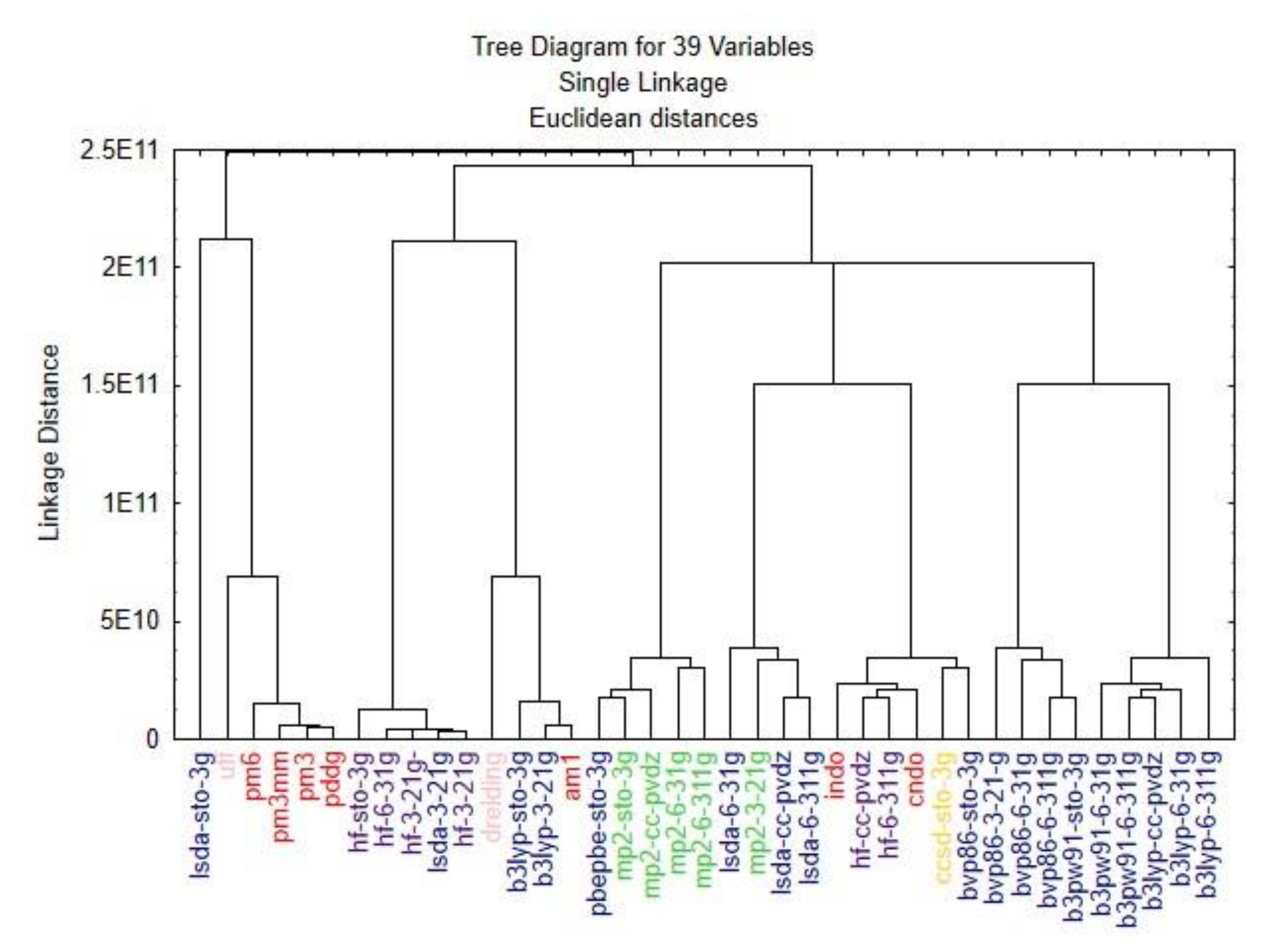
The cluster analysis dendrogram (Figure 5) shows the Euclidean distances between the 39 methods compared. The single linkage or nearest neighbour technique is one of the simplest hierarchical clustering methods. The Euclidian distance between the methods due to the large data set (3.538.080 variables) was very high. To compare these methods, the standardization of the linkage distance was chosen on the X-axis. (Dlink/Dmax) *100 represents the linkage distances (Dlink) divided by maximum linkage distance (Dmax).

The similarity between the optimization methods varies between the basis sets used. After obtaining the results of the PCA and clustering analyses, a classification can be made within the several different groups. The difference between the optimization methods was minimal; the tree clustering shows the relationship among them. For an extensive analysis, the data should be selected from different groups to obtain various results from multiple points of view.

Several studies use hybrid methods in their analysis [26,27,28] in order to obtain considerably better results. Davidson and Feller [28] in 1986 described a few criteria upon which a selection of the basis sets could be made, although since then many other methods have been introduced in computational chemistry. Because different theoretical methods and molecular properties have different basis set demands, different computer architectures and algorithms have different efficiency requirements, and the desired accuracy varies with the application, it is not possible to design one ‘optimum’ basis set.

Cramer [29] discussed the evolution of basis sets from the most widely used split-valence basis sets, such as 3-21G, 6-21G, 4-31G, 6-31G, and 6-311G [30], to modern examples of basis sets, such as cc-pCVDZ, cc-pCVTZ, etc. [31]. Comparing all the sets of comparisons, it is evident that the geometries for the molecules containing second-row elements are considerably more difficult to predict accurately than those for simpler organics. For example, it was found that AM1 is less successful when extended to these species than PM3 [32]. Furthermore, DFT methods feature limitations, such as different trends and high error accuracy [33].

The effort to determine the ‘best’ combinations of methods and basis sets that produce statistically good results for certain molecules and properties has become especially pronounced with the proliferation of the modern methods. Geometry optimization and energy minimization are fundamental tasks in molecular modelling and drug design. The failure to minimize energy and/or optimize geometry is directly converted to wrong molecular descriptors [34].

Because we used a very large data set, the results are more explicable if we divide them into different subgroups. After we performed the cluster and PCA analyses for every subgroup the following results were obtained.

For the semi-empirical methods, two principal components explain most of the data (Figure 6), and thecluster analysis showed the same tendency. The results can be divided into three main groups: am1; indo, cndo; and pm6, pm3mm, pm3, pddg. In conclusion, if we use one method from each group, this should be enough to describe our data.

For the Density Functional Theory methods, the statistical analysis looks a little different, because the dataset was larger this time. Most of the analyzed methods were part of this family.

Figure 7 demonstrates that the DFT methods are similar to each other, but also some ‘outlier’ methods can be observed. The methods can be divided into four major groups, and three methods, which are positioned separately.

In the Møller–Plesset Perturbation Theory methods, one principal component was identified (Figure 8). The methods are divided into two main groups, with one (mp2-3-21g) remaining a basis set.

The most widely used optimization calculation is the Hartree–Fock method. Based on our analysis, we identified two principal components (Figure 9) and two main groups.

The other methods, which are part of Coupled-Cluster Theory and Molecular Mechanics, could not be analysed separately because of the small dataset they represented. One method (CCSD) in Coupled-Cluster Theory and two methods (UFF, Dreiding) in Molecular Mechanics Theory did not reveal statistical significance if we analysed them alone. They are included in the first analysis, where all the methods are examined.

We performed another statistical analysis: the Single-Factor ANOVA test.

The reason for performing ANOVA was to see whether any difference existed between the groups for particular variables. The null hypothesis states that there was no significant difference between the methods analysed, based on the molecular descriptors calculated.

The p-value was 0.9995 > 0.05, so we accepted the null hypothesis, and concluded that there were no significant differences between the methods. In the Figure 10, the results of the ANOVA indicate that we cannot reject the null hypothesis.

4. Conclusions

In conclusion, we can state that the size of the basis set does not reflect its applicability in different circumstances. It is not possible to find the best basis set, only a couple of basis sets that fit our dataset. If we use different basis sets we obtain different results. Therefore, care must be taken to select the correct basis set. What makes the difference in results are the different selections and the correct use of optimization methods.

To find the best geometry optimization method to use in different situations, we must know are related. Two similar methods excluded each other in the analysis because they provided almost the same results. The results of our analysis show the correlation and the degree of relationship between the methods studied. The reclassification of the 39 examined methods facilitates the selection of the best basis sets for different study areas.