Temporal Degree-Degree and Closeness-Closeness: A New Centrality Metrics for Social Network Analysis

Abstract

In the area of network analysis, centrality metrics play an important role in defining the “most important” actors in a social network. However, nowadays, most types of networks are dynamic, meaning their topology changes over time. The connection weights and the strengths of social links between nodes are an important concept in a social network. The new centrality measures are proposed for weighted networks, which relies on a time-ordered weighted graph model, generalized temporal degree and closeness centrality. Furthermore, two measures—Temporal Degree-Degree and Temporal Closeness-Closeness—are employed to better understand the significance of nodes in weighted dynamic networks. Our study is caried out according to real dynamic weighted networks dataset of a university-based karate club. Through extensive experiments and discussions of the proposed metrics, our analysis proves that there is an effectiveness on the impact of each node throughout social networks.

1. Introduction

The research of centrality metrics dates to the 1940s and has been carried out in a variety of fields, including geography [1], psychology [2], and others. Social networks have recently been gaining increasing interest from researchers. With the growth of the popularity of complex social networks, many approaches have been developed to investigate and analyze these networks [3,4]. Analysis of the Social Network (SNA) [3,5,6,7,8,9] is an important method for the study of relationships between individuals. This includes research on social systems, social roles, role analysis, and a variety of other topics. One of the most difficult difficulties in the study of social networks is identifying the most important members of the network. The metric of centrality is used to determine the importance of a node’s placement in a network [10,11,12,13]. High centrality ratings define actors in networks with the most structural meaning, and these individuals are expected to play a prominent part in both simulated and real-world behaviors. Most models assume that networks are static, and that they are represented as a graph of nodes connected by edges [14]. The size of the gigantic component, which represents the size of the largest network component in a particular network following attacks, is often used in network science investigations. As a result, the size of the huge component as a measure of network resilience predicts the extent of fault tolerance in a given network based on the number of topological connectivity [15].

In reality, however, several networks are dynamic. New nodes are added to the graph, existing nodes are deleted, and edges appear and disappear. While various static centrality metrics have been established and are widely utilized for SNA, dynamic measures are a relatively new research area. Several extensions to the dynamic case of current static centrality metrics have been introduced in recent years. Many marketing apps tried to take advantage of social networks or media by targeting populations with simple centrality metrics like degrees, betweenness, or proximity [16]. Wan et al. introduce various existing centrality metrics and discuss their applicability’s in various networks. In addition, a large-scale simulation study is conducted to show and examine the network resilience of focused attacks using the surveyed centrality metrics in four different network topologies [17].

Tabirca et al. [18] proposed an algorithm depended on an adapted computation to dynamic shortest paths to calculate certain dynamic indices (dynamic graph, dynamic closeness, dynamic betweenness and dynamic stress). By depicting the network as a time series, D. Braha and Y. Bayram [19] show how degree centrality evolves. Lalou et al. [20] discussed new research that has addressed the difficulty of finding essential nodes in a network. The focus of this research was on theoretical complexity, exact solution algorithms (rather than centrality measurements), approximation strategies, and heuristic approaches. The authors demonstrated novel complexity results of algorithms that were enhanced based on interactions between variations. Federico et al. [21] established a new centrality metric termed change centrality, which evaluates how central a node is in terms of network changes. Until recently, the models and analytical methods used to characterize dynamic network behavior were constrained. It is simple and common to examine static network snapshots independently and use the average attributes of all snapshots, for example, a feasible technique to quantify the topological significance of a node over time is to use the average value of all static snapshots on the node’s centrality. Such dynamic analysis is limited, however, because temporal pathways that traverse many temporal snapshots are omitted. Pathways between nodes can be created in dynamic graphs by sewing partial paths between temporal snapshots. Tang et al. [22] proposed temporal centrality measures based on temporal routes in order to effectively quantify the importance of a node in a complex network. Furthermore, Kim and Anderson [23] enhanced the Tang idea by introducing a new model termed a time-ordered graph that may convert a dynamic network to a static network with directed flows. The temporal description for the centrality metrics of degree, betweenness and closeness according to that model is also provided [23]. In several networks, the links are not just binary entities, whether present, yet have linked weights that log their relative strengths to each other.

Weights are assigned to ties between nodes in weighted networks. Ties frequently have an inherent strength associated with them that distinguishes them from one another. Weights have been assigned to tie strength. For weighted networks, a few centrality measures have been developed, such as those in [24,25,26]. While many social networks are dynamic and weighted, this paper explains the meaning of temporal degree, temporal closeness and temporal degree-degree centrality for such networks, there is a proposal for a new centrality measure (temporary Closeness-closeness centrality) to have a better approach understanding of the significance of nodes in weighted dynamic networks.

2. Related Work

The purpose of network centrality diagnostics is to determine the relevance of nodes. The meaning of a node may have depending on the application. Different definitions have been proposed, and as a result, several metrics of network centrality, such as degree, closeness, and betweenness centrality [5], have been presented. The number of links occurring upon a node is characterized as degree centrality, which focuses on the level of communication activity (i.e., the number of ties that a node has). The degree can be expressed in terms of a node’s immediate danger of catching something that is passing over the network (like a virus, or information). The formal definition of a node’s degree centrality v is

$$c_v\left(v\right)=\frac{\mathrm{deg}\left(v\right)}{N-1}.$$

(1)

where N is the total number of nodes in the network and deg(v) is the number of its linkages. Closeness Centrality believes that nodes with a short distance to other nodes can spread information via the network very effectively. The centrality of a node’s proximity v can be formalized as

$$c_c\left(v\right)=\frac{N-1}{{{\displaystyle \sum }}_{i\ast u}d\left(u,v\right)}$$

(2)

where d(u,v) refers to the shortest-path distance between actors v and u. Although the using time-ordered weighted graph in this paper, we can often find no temporal path from v to u, the distance between v and u is ∞. Therefore, the distances are inverse after summation, according to Equation (2), and the summation of the infinite number is infinite. Opshal [27] proposed the closeness centrality as the sum of inverse distances to all other nodes instead of the inverse of the sum of distances to all other nodes because the limit of a number divided by infinity equals zero:

$$c_c\left(v\right)=\frac{{{\displaystyle \sum }}_{\mathrm{M}}\frac{1}{d\left(u,v\right)}}{N-1}$$

(3)

For u,v weighted networks, where edges are either present or missing and have no weight attached, many centrality measures [10,11,12] have been implemented. Designing centrality measures for weighted networks whose weights convey information has become increasingly important. Barrat et al. [25] added degree centrality to weighted networks. The weights related to the edges connected to a vertex are added together to form a total. Opsahl et al. [28] have proposed a new generation of vertex centrality. Weighted network measures take into account both edge weight and the number of vertex-associated edges. Furthermore, Abbasi and Hossain [29] presented new hybrid centrality measures (Degree-Degree, Degree-Closeness, and Degree-Betweenness) that combine existing measures (Degree, Closeness, and Betweenness). A generalized set of weighted network measurements has also been proposed [29]. Tang et al. [22] proposed temporal centrality measures based on temporal routes to efficiently assess the importance of a node in a dynamic network, as many networks are dynamic in that their topology changes over time. In addition, Kim and Anderson [23] expanded on Tang’s concept by introducing a new time-ordered graph model. According to that paradigm, the temporal definitions for degree, betweenness, and closeness centrality metrics are also provided [23]. A. Meligy et al. [30] refined Kim’s model so that it could be applied to weighted networks properly; this model is known as the time-ordered weighted graph. While many social networks are dynamic, this research uses a time-ordered weighted graph model to suggest a generalized definition of temporal degree and temporal closeness for weighted networks. For dynamic networks, this approach is used to improve the Degree-Degree measure [29] (Temporal Degree-Degree). Finally, a new centrality measure (Temporal Closeness-Closeness) is developed to improve the closeness centrality measure’s outcomes. The dynamic weighted network and the time-ordered weighted graph are described in Section 3 and Section 4. Then, in Section 5, we present our proposed measures.

3. Dynamic Weighted Network

A dynamic network is one in which the topology changes over time as edges are added or removed. Consider the time during a network is finite from t_min = 0 to t_max = T. A dynamic weighted network $G_{0, T}^G=\left(V, E_{0,T}, W\right)$ on a time interval [0, T] includes a set of vertices V, a set of edge weights W, and a set of temporal edges $E_{0,T}$. The temporal edge (u,v)$\in$ E_0,T and its corresponding weight w_uv exist between vertices u and v on [i,j] such that i ≤ t_max, j ≥ t_min. A sequence of snapshot is used to represent dynamic networks, where for each snapshot consider $\Delta t$ as time interval (size of snapshot). A dynamic network can be represented as a series of graphs $G_{t_{min}}, G_{t_{min+\Delta t}}\dots , G_{t_{max}}$. 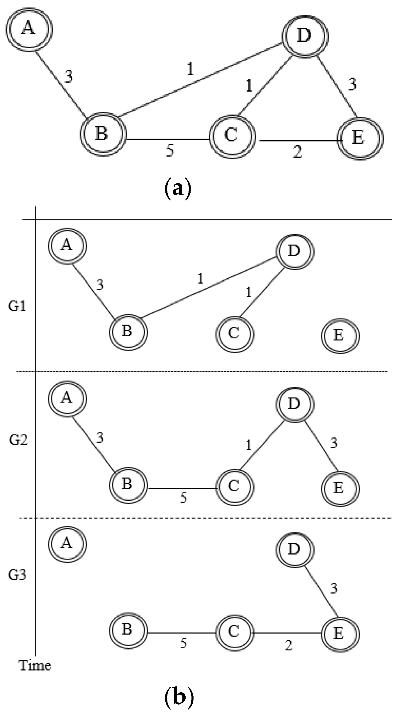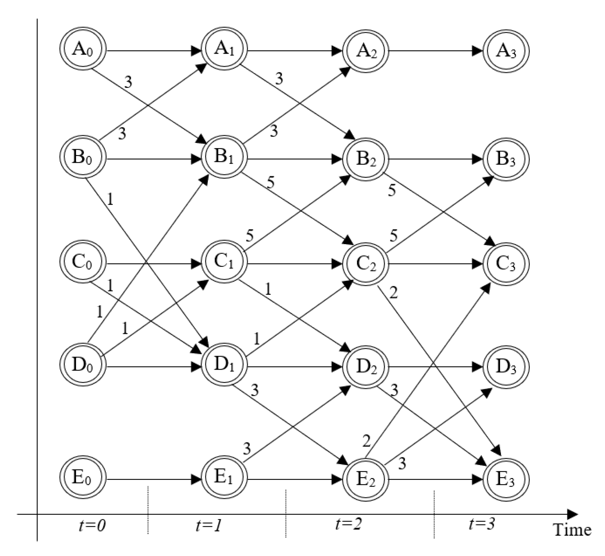Then, G_t represents the aggregated graph with v, w, and E_t where v is a set of vertices, w is a set of weights, and E_t is a set of edges, where an edge with its weight w_uv exists in G_t only if a temporal edge (u, v) ∈ E_0,T exists between vertices u and v on a time interval [i,j]. Consider the following example at t_min = 0, t_max=3 and $\Delta t=1$,

Table 1. Example of dynamic weighted network edges.

Temporal Edge	Time Interval	Edge Weight
(B,D)	[1,1]	1
(A,B), (C,D)	[1,2]	3,1 respectively
(B,C), (D,E)	[2,3]	5,3 respectively
(C,E)	[3,3]	2

shows how a dynamic network with a set of temporal edges and weights may be represented as an aggregated graph with all edges aggregated into a single graph, G_t as in Figure 1a, and the series of static networks, G₁, G₂, and G₃ as in Figure 1b.

Aggregate over all edges, as shown in Figure 1a, loses a lot of temporal information that might assist describe the dynamic network structure, such the frequency of events and the time gap between them. It is difficult to directly analyze the temporal aspects of a dynamic network, as demonstrated in Figure 1b by a representation of the time series derived from network snapshots. Therefore, we may assume that all temporal information cannot be represented by time series representation.

4. Time-Ordered Weighted Graph

To get all network connection information, a time-ordered weighted graph is formed as illustrated in Figure 2. There is more information on the events mentioned in Table 1 in this graph. Let Time-ordered weighted graph G = (V,E,W) is a directed weighted graph with a vertex v_t for each v ∈ V and t ∈ {0, 1, …, n}; let edges from u_t−1 to v_t and from v_v−1 to u_t with the weights w_ut−1vt, w_vt−1ut associated to those edges, respectively. It has edges from v_t−1 to v_t for all v ∈ V and t ∈ {0, 1, …, n}. The weights in this paper are considered as natural numbers. The definition for the proposed measures for a dynamic weighted network is displayed based on G = (V, E, W).

5. Proposed Centrality Measures

Let us consider a time-ordered weighted graph with varying time, as illustrated in Figure 1b, the definitions of Temporal degree, Temporal closeness, Temporal Degree-Degree, and Temporal Closeness- Closeness centrality are presented with the results of these metrics on the illustrative example.

6. Temporal Degree Centrality

Barrat et al. [25] defined degree centrality for weighted static networks as the total of the weights associated to the edges connected to a vertex, referred to as node strength. This measure is expressed as follows:

$$C_D^w={\displaystyle \sum }_u^N{w}_{vu}$$

(4)

Node strength is a blunt metric, according to Opsahl et al. [28], as it only considers a node’s overall degree of network participation, not the number of other nodes to which it is connected. In order to describe the degree centrality as the product of the number of nodes to which a node is attached, both the node degree and its strength were combined, and the average weight of these nodes was adjusted by a tuning parameter, a, which expresses the value of the number of ties in relation to the tie weights:

$$C_D^{wa}\left(v\right)=k_v\times \left(\frac{s_v}{k_v}\right)=k_v^{1-a}\times s_v^a$$

(5)

where k_v is the number of direct neighbors of v, s_v is the node strength and a is a tuning parameter with a positive value. The value of a can be illustrated as shown in

Table 2. Different values of a is illustrated.

Value for a	Measure Outcome
a = 0	equal to number of nodes in connection
a = 1	equal the node’s strength
0 < a < 1	a high degree is taken as favorable
1 < a	a low degree is favorable

.

a = 0.5 is chosen. In addition, Equation (5) is generalized for the directed networks by Opshal et al. [28] such that the in-degree and out-degree centrality can be formalized, respectively, as follows:

$$C_D^{wa}\left(v\right)=k_v^{in}\times {\left(\frac{s_v^{in}}{k_v^{in}}\right)}^a$$

(6)

$$C_{D out}^{wa}\left(v\right)=k_v^{out}\times {\left(\frac{s_v^{out}}{k_v^{out}}\right)}^a$$

(7)

The temporal degree TD_wa (v) for a node v ∈ V in a weighted network on a [i,j] is the summation of the node’s degree centrality at each time step, such that 0 ≤ i ≤ i ≤ n. The node’s degree centrality at each time step is the total number of outbound edges from (or inbound edges to) v; disregarding the self-edges from v_t−1 to v_t; multiplied by the weight associated to the edges adjusted by α, for all t ∈ {i + 1, …j}. Then, the temporal degree centrality of a node v on [i,j] can be formalized as follows:

$$T{D}_{wu}\left(v\right)={\displaystyle \sum }_{i=1}^i{\left(\mathrm{deg}(v_t\right)}^{\left(1-u\right)}\times w^a)$$

(8)

where deg (v_t) is the number of out-links (or in-links) of v at each time step and $w$ is the total weight attached to the outgoing (or incoming) ties of v at each time step.

7. Temporal Closeness Centrality

The centrality of closeness assumes that nodes with a short distance to other nodes can disperse knowledge across the network very productively. The closeness centrality measure depends on the length of the shortest paths among nodes in the network. The shortest path length in binary networks is the shortest number of connections between two nodes, either directly or indirectly. Several attempts have been made to find the shortest paths in weighted networks. Newman [26] and Brandes [31] proposed the distance between two nodes as the minimum number of the sum of the inverted weights as follows:

$$d^w\left(u,v\right)=\left(\frac{1}{w_{vh}}+\dots +\frac{1}{w_{uh}}\right)$$

(9)

where h are intermediary nodes on paths between node v and u. The authors have found that the algorithms of Newman and Brand, when used to find the shortest distance between two nodes, are not affected by the number of nodes on the shortest path between two nodes. By considering the number of intermediate nodes, Opshal et al. [28] extended the shortest path algorithms and specified the length of the shortest path between two nodes as follows:

$$d^{wa}\left(u,v\right)=(\frac{1}{{(w_{vh})}^a}+\dots +\frac{1}{{(w_{uh})}^a})$$

(10)

Kim and Anderson [23] defined the temporal shortest path length, for binary dynamic networks, according to the time-ordered graph, from node v to node u on [i, j] where 0 ≤ i ≤ j ≤ n as d(v,u) = min i < l ≤ δ (v,u), where d(v,u) is the shortest path distance from v to u in a static graph. The definition of Opshal’s shortest distance is extended in this paper to the time-ordered weighted graph to describe the temporal shortest path distance for weighted networks between two nodes over a time on [i,j] as

$$d^{wa}\left(u,v\right)=\left(\frac{1}{{(w_{vh})}^a}+\dots +\frac{1}{{(w_{uh})}^a}\right)$$

(11)

The proposed temporal distance (Equation (9)) is used to define the closeness centrality of a node in dynamic weighted network. Temporal closeness centrality TC_wa(v) of a node v in a weighted network on [i,j] where 0 ≤ i ≤ j ≤ n is the sum of inversed temporal shortest path distances to all other nodes in v for each time interval in {[t,j]: i ≤ t < j}. Then, the temporal closeness centrality of a node v on the interval [i,j] is defined as follows:

$$T{C}_{wa}\left(v\right)={{\displaystyle \sum }}_{i\le t\le j}{\displaystyle \sum }_{u\in V}\frac{1}{d^{wa}\left(v,u\right)}$$

(12)

If there is no temporal path from v to u on [t,j], d_wa(v,u) is defined as ∞. Also, we assume that the weight of the self-edges is 1.

8. Temporal Degree-Degree

Abbasi and Hossain [29] have expanded the traditional measures of centrality and the implementation of modern hybrid measures to represent the importance of a node through the importance of its direct neighbors in binary and weighted networks. Degree-Degree centrality is one of these hybrid steps, which demonstrates the actors who are related to the actors who are better associated. Therefore, it reveals an actor’s success centered on the popularity of his immediate neighbors. Degree-Degree is applied to be suitable for dynamic networks in this paper and is called Temporal Degree-Degree. First, for each node, the Temporal Degree TD_wa is computed. Then, the hybrid centrality measure of a node is determined by summing the degree multiplied by the weight of the edge between the node of each direct neighbor that defines as follows:

$$TD{D}_w\left(v\right)={\displaystyle \sum }_{t=1}^j{\displaystyle \sum }_{u\in V}(C_D^{wa}\left(u_t\right)·w\left(v_{t=1},u_{t }\right))$$

(13)

where u is direct neighbor of v and $w$ (v_t−1, u_t) is the weight of the edge between v_t−1 and u_t.

9. Temporal Closeness-Closeness

Closeness centrality is defined as the efficiency of an actor in the spread of information throughout the network. If an actor is directly linked to actors with high values of centrality closeness, then this actor will have more accessibility and effectiveness in spreading information. Then, the main issue is how to determine the actor who is better close to all other actors. A new hybrid centrality measure based on closeness centrality, Temporal Closeness-Closeness centrality, is proposed in this paper. First, the temporal closeness centrality for all direct neighbors is computed to calculate the Temporal Closeness-Closeness measure. Temporal Closeness-Closeness (TCC_w(v)) is defined as follows:

$$TC{C}_w\left(v\right)={\displaystyle \sum }_{u\in V}{\displaystyle \sum }_{1\le t<j}\frac{1}{d^{wa}\left(v,u\right)}·T{C}_{wa}\left(u\right)$$

(14)

10. Results and Discussion

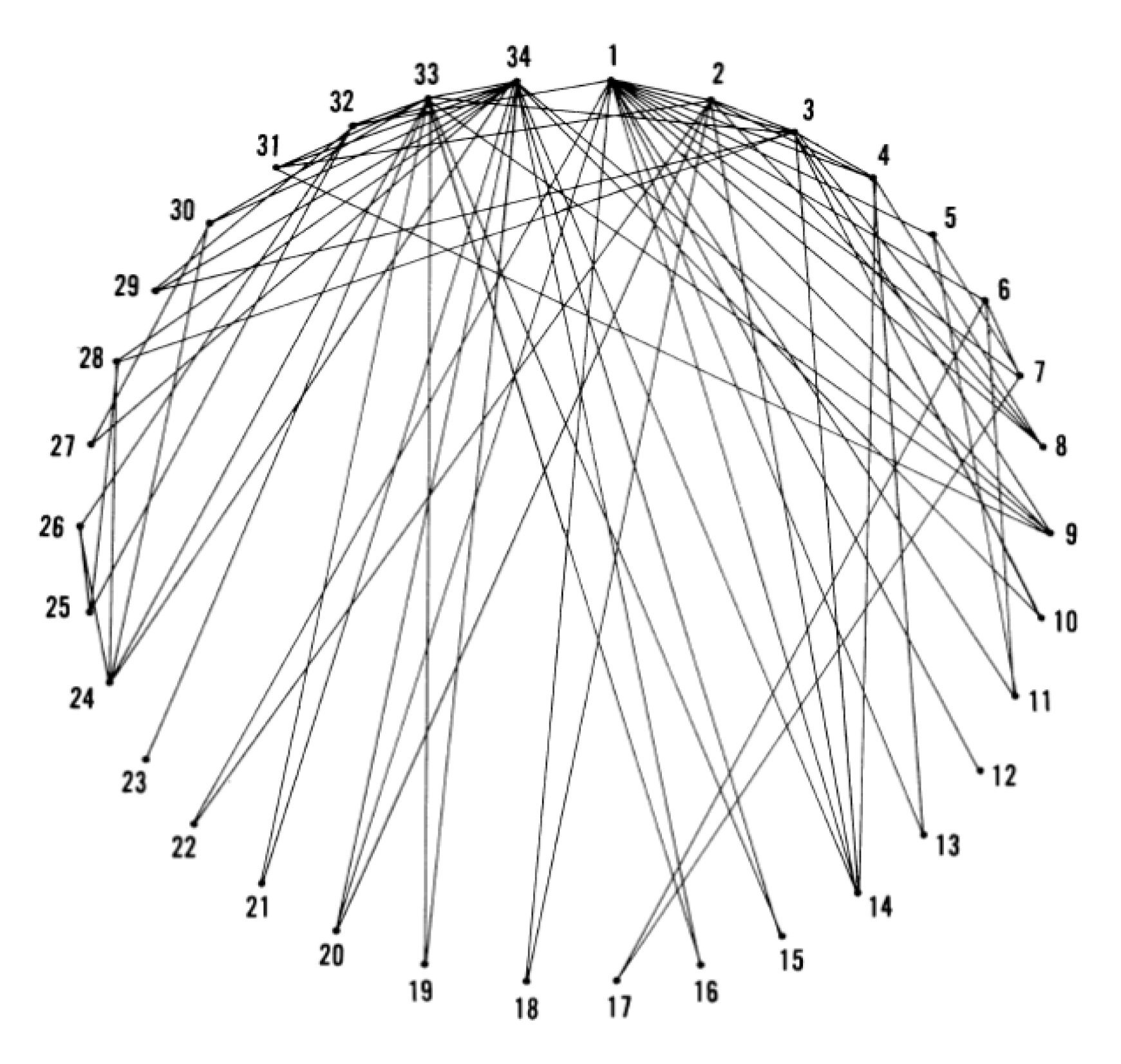
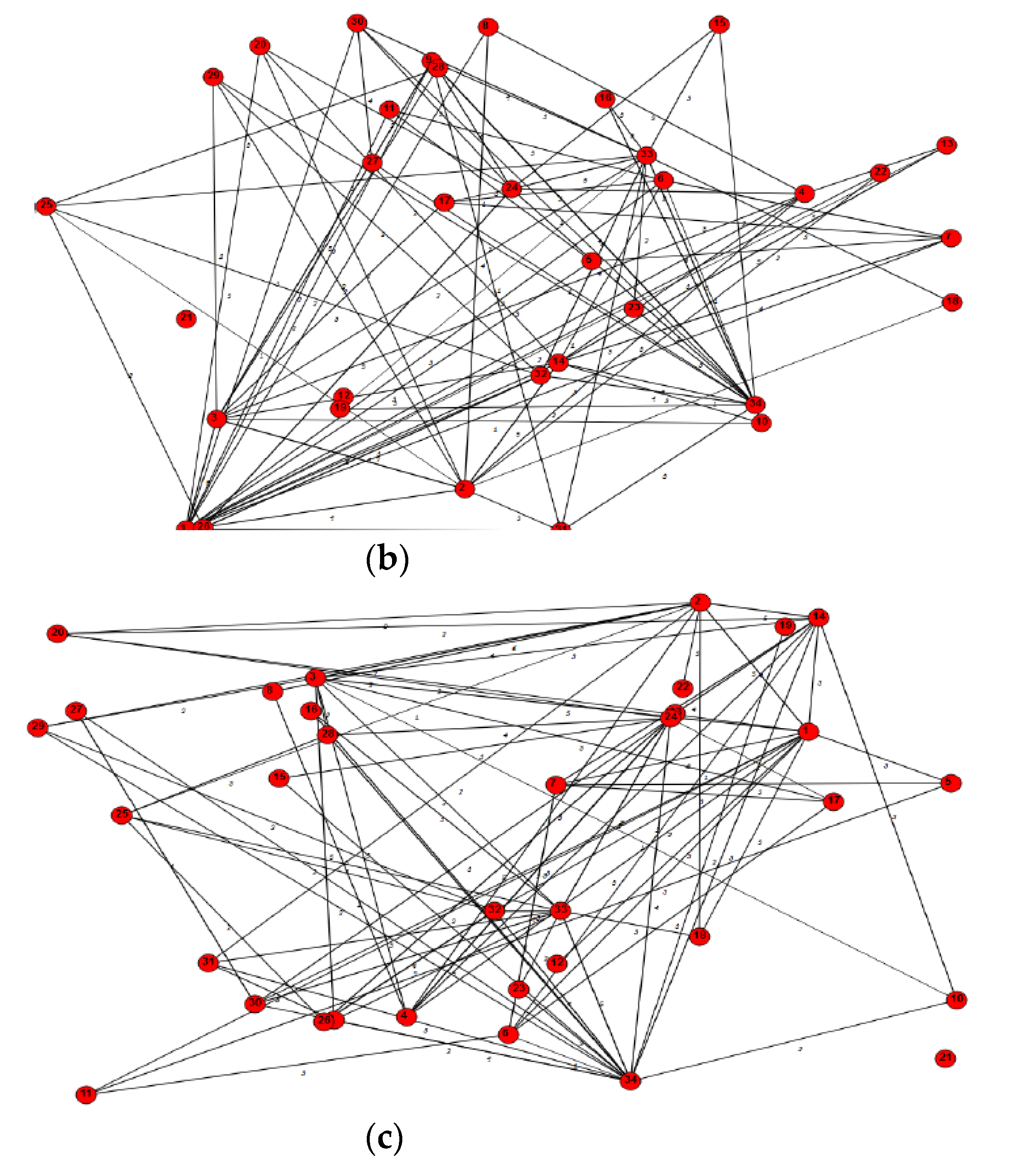
The significance of the proposed measures on real dynamic weighted networks is presented in this section. A dataset [32]—a university-based karate club—is used to test the proposed measure. Wayne Zachary gathered this database from members of a university karate group. From 1970 to 1972, the karate club was monitored for three years. The club had between 50 and 100 members during the observation period, and its activities included social events (parties, dances, banquets, etc.) as well as regularly scheduled karate instruction, as indicated in Figure 3.

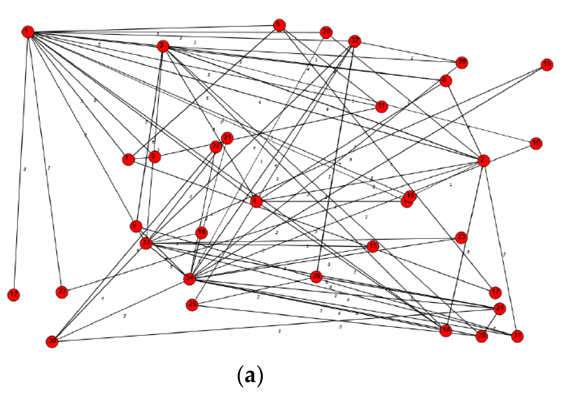
In the graph, there are just 34 persons. The group had over 60 members at the time, and outside of meetings and classes, none of the 26 members who were not represented communicated with other club members. These people are not included because they would only be disconnected points in the graph. An edge appears in this graph if two entities were repeatedly seen interacting outs. However, the aim of this dissertation is to suggest centrality measures for weighted dynamic networks. It means we’ll have to change this dataset to meet our objectives. Therefore, using the SocNetV 1.8 program, we built a dynamic network out of this dataset by taking two more random snapshots as shown in Figure 4. The number on the edge shows the strength of the corresponding edge, namely the number of interactions between two actors.

On this dataset, the Temporal Degree (TD) centrality metric is used to investigate the actor with the most friends and the highest number of situations between him and his friends. As we have mentioned in the methodology about the parameter α, if this value is between 0 and 1, a high degree (i.e., a large number of linkages) is considered advantageous. A low degree (i.e., a small number of connections) is preferable if it is set above 1. In this work, we will concentrate on the nodes which have high number of ties. Thus, we have computed the TD using α = 0.5.

Table 3. Temporal Degree centrality and Temporal Degree-Degree centrality of all members.

Rank	Individual Number	TD	Individual Number	TDD
1	34	83.411	3	921.0236
2	1	74.0844	34	896.116
3	33	64.0574	1	865.5355
4	3	53.943	33	861.3614
5	2	53.6788	2	788.0057
6	14	45.5513	14	781.2183
7	24	44.1881	24	697.923
8	4	35.7695	9	668.5796
9	32	33.6749	32	628.159
10	6	27.6823	4	612.6358
11	9	26.1851	31	506.3155
12	7	25.6502	28	469.126
13	30	24.5316	30	453.9031
14	31	21.9268	8	394.1019
15	28	21.6333	7	375.6863
16	26	19.4422	6	367.7755
17	25	18.7247	26	355.1395
18	8	16.1489	16	347.4907
19	17	16.1132	15	288.7119
20	29	15.5563	20	269.0651
21	20	15.1867	29	263.6679
22	5	14.6969	23	249.9422
23	11	14.6969	13	215.1224
24	13	12.0246	5	210.7565
25	16	11.225	10	199.9653
26	15	11.2235	17	186.5505
27	10	10.9348	11	186.3138
28	27	10.3923	27	178.9725
29	18	9.5206	25	172.6506
30	23	9.4868	22	171.3696
31	22	7.0711	19	152.3937
32	19	6.3132	18	149.6821
33	12	3.4641	21	95.8331
34	21	2.8284	12	78.6893

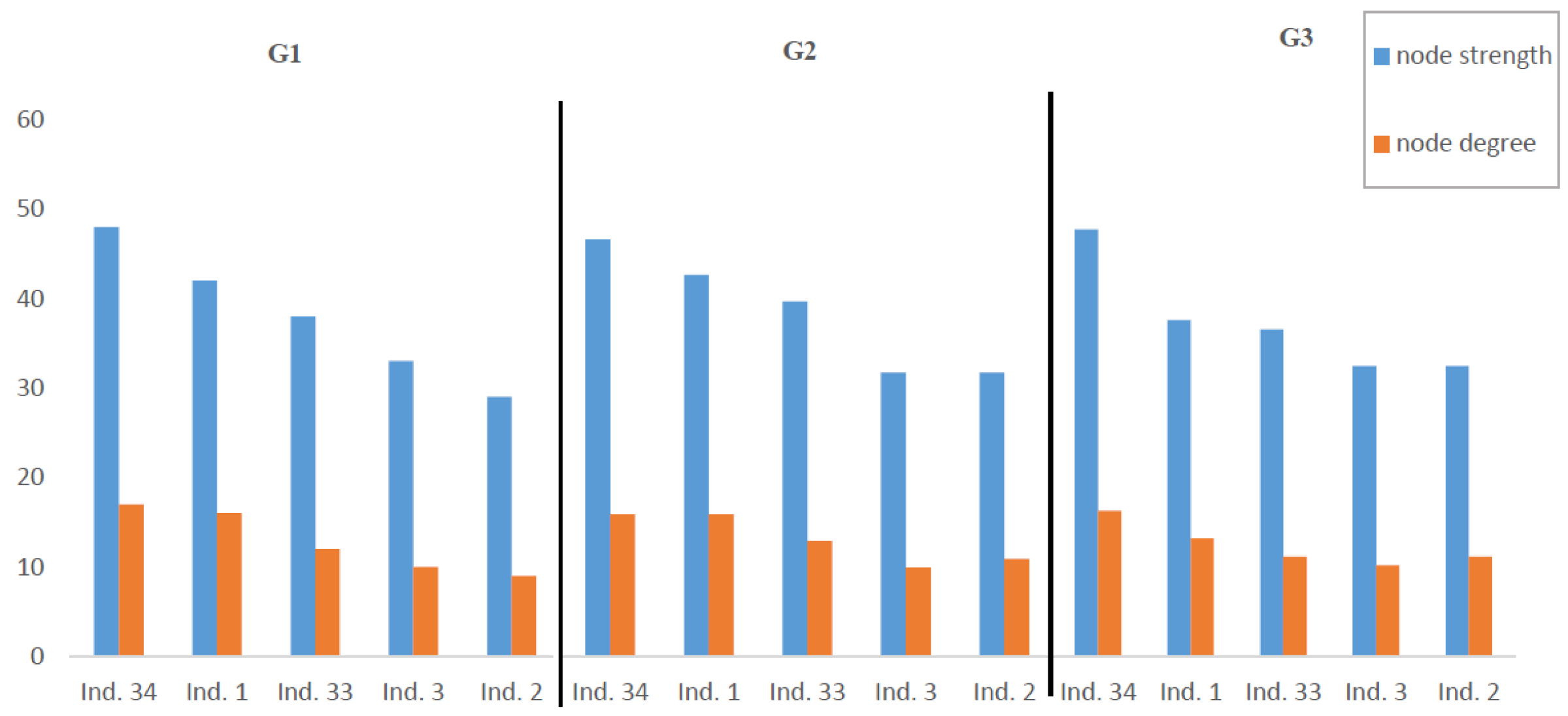
ranks the 34 members according to the temporal degree and temporal degree-degree centrality values. Looking at the most central individuals in column 2 of Table 3, we can see that individual 34 is the most central member as he is connected to the most people (17 members at the first snapshot and 16 members at the second\third snapshots) and has the highest number of situations between his friends (48 situations at the first snapshot and 47 situations at the second\third snapshots). Furthermore, Individual 1 comes in second place as he has 16 friends with 42 situations at first snapshot, 16 friends with 43 situations at second snapshot, and 13 friends with 37 situations. To give more clarification about the Temporal Degree results, Figure 4 shows the node strength and the degree of the top five individuals at each time step. As shown in Table 3, the rank of individual 3 changes considerably when measuring TD and TDD. He ranks fourth when measuring TD as he has less friends, and the number of situations he shared with others is relatively low as compared to individuals 34, 1, and 33. On the other hand, he becomes the most central one when measuring TDD as he connects with many individuals who have high degree over time. In addition, some individuals (like individuals 2, 14, 24, 32, 30, and 27) maintain a relatively stable ranking.

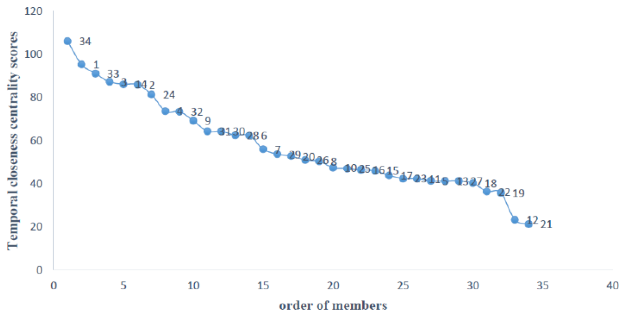
To obtain the actor who has a short distance to other actors in the network, temporal closeness centrality is applied. More specifically, we want to find the actor who has the minimum number of intermediary individuals between him/her and other actors. To achieve this goal, we have measured TCCL with α = 0.5. The ranking estimated closeness centrality scores of all social network members are shown in

Table 4. TCL and TCCL centrality values of all individuals.

Rank	Individual Number	TC	Individual Number	TCC
1	34	106.1934	34	65.4851
2	1	95.4326	1	59.0754
3	33	91.1215	33	58.3442
4	3	87.3446	3	57.9846
5	14	86.2297	14	56.0769
6	2	86.054	2	55.5116
7	24	81.4526	24	53.0075
8	4	73.7464	4	48.9706
9	32	73.5296	32	48.0931
10	9	69.2996	9	47.4077
11	31	64.4295	31	43.527
12	30	64.3846	30	42.6416
13	28	62.5983	28	42.397
14	6	62.4724	6	39.3179
15	7	56.0802	29	36.4985
16	29	53.8387	7	16
17	20	52.8529	20	35.4313
18	26	51.06	26	34.4055
19	8	50.4763	8	33.6287
20	10	47.5403	10	32.6459
21	25	47.1532	16	32.6001
22	16	46.5431	25	31.6699
23	15	46.0769	15	31.4502
24	17	43.9576	23	29.501
25	25	42.4557	17	29.4142
26	11	42.4119	13	28.5572
27	5	41.4289	18	28.361
28	13	41.4183	27	28.0837
29	27	41.409	11	26.9834
30	18	40.3926	5	26.7691
31	22	36.5563	19	24.4175
32	19	35.8629	22	24.1237
33	12	23.382	12	16.0608
34	21	21.321	21	13.8925

and Figure 5.

Individual 34 has direct connection to many other actors over time. Therefore, most of his path lengths are all very short, namely, he has the minimum number of intermediary nodes between him and the other nodes. Thus, actor 34 has high temporal closeness centrality. Furthermore, individual 21 has not any path between him and other individuals at second and third snapshots. Therefore, he is the farthest one (as in second column in Table 4 and Figure 6) because he is isolated in these snapshots. To find the actor who has short paths to actors who have high closeness centrality, we calculated the temporal closeness-closeness for all individual as in the fourth column of Table. Unfortunately, the results of TCCL does not differ significantly from the results of TCC. That is because the topology of this network has little changed over time. Thus, the distances between actors changed at few positions in the network.

To illustrate the results of TCCL measure, we have changed the topology of this network by creating other snapshots which have many changes. Then, we computed this measure using these new snapshots.

Table 5. TCL and TCCL centrality values of all individuals in the modified network.

Rank	Individual Number	TC	Individual Number	TCC
1	33	0.9107	34	0.7349
2	3	0.905	1	0.6462
3	1	0.885	33	0.6424
4	34	0.8755	3	0.6081
5	24	0.8754	14	0.5963
6	32	0.796	2	0.595
7	2	0.7735	24	0.5705
8	9	0.7662	32	0.5246
9	14	0.7329	4	0.5219
10	26	0.7188	9	0.5005
11	4	0.7085	30	0.4634
12	31	0.7002	31	0.4618
13	28	0.6932	28	0.4518
14	30	0.6900	6	0.4246
15	7	0.6654	29	0.3871
16	6	0.6387	7	0.3771
17	8	0.6331	20	0.3748
18	11	0.3696	26	0.3696
19	16	0.6193	8	0.3541
20	27	0.6192	25	0.3437
21	23	0.6184	10	0.3405
22	29	0.6168	16	0.3405
23	21	0.6115	15	0.3344
24	25	0.6000	17	0.3151
25	5	0.5919	23	0.3086
26	15	0.5614	18	0.2977
27	20	0.5415	27	0.2957
28	13	0.5234	13	0.2931
29	10	0.5178	11	0.2892
30	18	0.5170	5	0.2888
31	22	0.5145	19	0.2579
32	19	0.5133	22	0.2554
33	17	0.4465	12	0.1689
34	12	0.3971	21	0.1507

shows the TCL and TCCL values for all actors in the modified network.

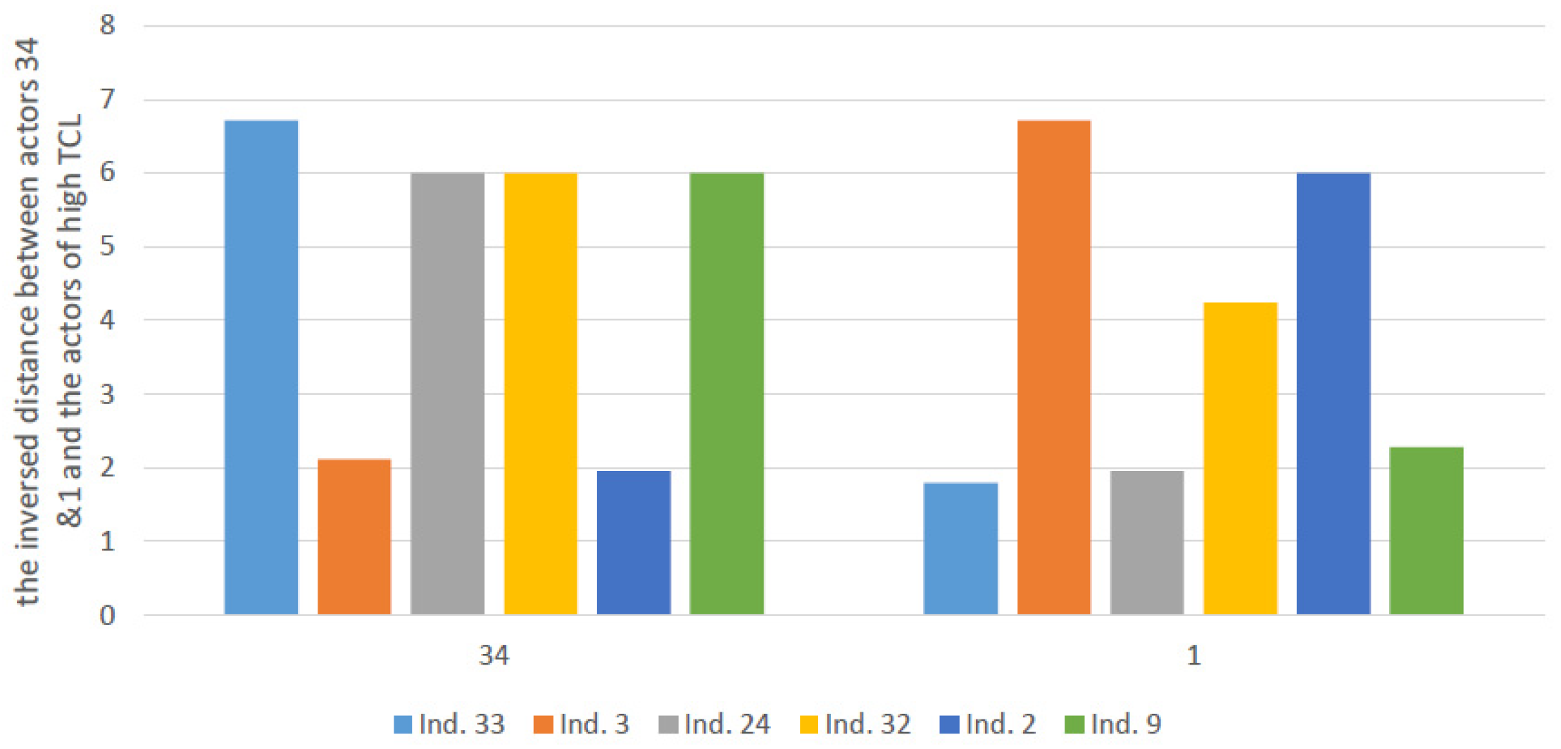
From the fourth column in Table 5, we have found that individual 34 and 1 are the top two individuals. That is because they have shortest paths to many individuals of high TCL values, i.e., individual 34 and 1 are the closest members to the members of high TCL values. In order to show that individual 34 and 1 are close to more actors of high TCL, Figure 7 shows how close each of individual 34 and individual 1 to some actors (like: 33, 3, 24, 32, 2, and 9) whose have high TCL values.

It is obvious from Figure 7 that individual 34 is closer to actors 33, 24, 32, and 9 than individual 1, i.e., individual 34 is close to more actors whose have high TCL than individual 3. That is because the distance between actor 34 and many actors of high TCL is short. Therefore, individual 34 can be considered as an actor who can help in spreading information in the network.

11. Conclusions

In this paper, a new hybrid centrality measure based on closeness centrality—Temporal Closeness-Closeness centrality—was proposed. The temporal closeness centrality for all direct neighbors was computed to calculate the Temporal Closeness-Closeness measure. The measure was based on time-ordered weighted graph model with Opshal’s algorithms for calculating degree centrality and the shortest distance in weighted networks. In a dynamic weighted network, a metrics was used to represent a node’s popularity and accessibility with respect to Temporal Degree, Temporal Closeness, Temporal Degree-Degree, and Temporal Closeness-Closeness. The temporary degree-degree described the nodes that were better connected to more nodes. Temporal closeness-closeness suggested a node’s accessibility dependent on its direct neighbors’ accessibility. As a future work direction, we need to develop metrics that based on closeness and degree to find new measure such as Closeness-Degree and Degree-Closeness. More comprehensive, diverse, larger, and real network topologies can be considered to obtain more meaningful findings to provide generalizable guidelines for selecting useful centrality metrics in each application.