Analysis of Asymptotic and Transient Behaviors of Stochastic Ratio-Dependent Predator–Prey Model

Abstract

In this paper, we focus on the asymptotic and transient dynamics of the studied ecosystem and measure the response to perturbation of the stochastic ratio-dependent predator–prey model. The method we use is mainly based on the Kronecker product and numerical simulation. Firstly, the mean-square stability matrix can be calculated from the Kronecker product, so as to compute three indicators (root-mean-square resilience, root-mean-square reactivity and root-mean-square amplification envelope) of the response to perturbation for the studied ecosystem. Since the above-measured amounts cannot be obtained explicitly, we use numerical simulation to draw the changing figures within the appropriate parameter range. Then we obtain some conclusions by comparing the numerical results. When perturbing any populations, increasing the disturbance intensity will reduce the mean-square stable area of the system. Ecologists can manage the ecosystem, reduce losses and maximize benefits according to the numerical results of the root-mean-square amplification envelope.

1. Introduction

The stability of an ecosystem has always been the focus of biologists and it involves many fields, such as the protection of the ecosystem, economic development, political management and so on. Traditionally, scholars are interested in the asymptotic stability of ecological models and have conducted several qualitative analyses and quantitative calculations. In previous studies, it is known that asymptotic stability can be characterized by resilience. In 1977, Pimm and Lawton [1] proposed the definition of resilience in a biological sense for the first time, which means the asymptotic decay rate of perturbations. Given a linearized (or linear) system

$$\frac{dx}{dt}=Ax$$

(1)

The resilience is calculated as $v_{\infty }=-\Re \left({\lambda }_{max}\left(A\right)\right)$,${\lambda }_{max}\left(A\right)$ is the eigenvalue of A with the largest real part. The greater the resilience, the faster the decay rate of the disturbance in the long run and the more stable the system. Although the long-term asymptotic dynamic behavior is significant, the short-term transient dynamic behavior also cannot be ignored. Some systems are ultimately stable; however, the trajectory of these systems may rapidly move away from the equilibrium in the early stage after being disturbed. For example, the pests that will eventually become extinct can surge in the beginning. The infectious diseases, which will be solved, can cause a large number of deaths at first. Therefore, if we only consider the final state and ignore the temporary behavior of the system, we will suffer serious losses.

In the past few years, scholars have made remarkable achievements in transient dynamics for the ecosystem. In 1997, Neubert and Caswell [2] introduced reactivity as a supplement to resilience, which means the maximum initial rate that a small perturbation can grow. It characterizes the instantaneous responses ($t\to 0$). The reactivity is denoted by $v_0={\lambda }_{max}\left(H\left(A\right)\right)$, $H\left(A\right)=\frac{A+A^T}{2}$ is the Hermitian part of the Jacobian matrix A. The equilibria is called reactive if $v_0>0$. The larger the reactivity, the more sensitive the system and the faster a perturbation can grow. When ${\lambda }_{max}\left(A\right)<0$ and ${\lambda }_{max}\left(H\left(A\right)\right)>0$, the system is eventually stable but reactive. This situation is possible and not accidental.

Resilience and reactivity describe two limits of solution behaviors $(t\to \infty$ and $t\to 0)$, but neither describes the transient behaviors between zero and infinity. Therefore, Neubert and Caswell [2] defined the amplification envelope $\rho \left(t\right)$. It is the maximum possible amplification that any initial-value perturbation could induce in a solution at time t, given by $\rho \left(t\right)=\parallel e^{At}\parallel$, where $\parallel e^{At}\parallel$ is the Euclidean matrix norm of $exp\left(At\right)$. In addition, the maximum value of $\rho \left(t\right)$ is denoted by ${\rho }_{max}=\underset{t\ge 0}{max}\rho \left(t\right)$. The time at which ${\rho }_{max}$ occurs is denoted as $t_{max}$.

Based on these conclusions, scholars further studied the resilience, reactivity and envelope amplification of ecosystems. Regarding resilience, Folke, Carpenter and Walker [3] had a heated discussion around resilience and put forward several significant concepts related to ecological resilience, such as adaptability, transformability, etc. In the same year, Hughes and Graham et al. [4] found that resilience played an important role in the management of marine ecosystems (such as coral reef systems), and proposed that we should learn how to avoid unnecessary phase transformations of ecosystems. In 2019, Wright [5] proposed a model of social resilience and sustainable development in the 21st century from the lessons of historical ecology. For reactivity, Snyder [6] analyzed what makes the ecosystem reactive. Then, Vesipa and Ridolfi [7] also focused on the short-term dynamics of long-term stable and reactive ecosystems in 2017. Taking a seasonal forced prey–predator model as an example, it is proved that seasonality can greatly affect the transient dynamics of the system.

In 2014, Evelyn Buckwar and Conall Kelly [8] extend the above measure indicators to stochastic cases for a perturbed predator–prey model, which are called root-mean-square resilience, root-mean-square reactivity and root-mean-square amplification envelope. Since ecosystems exist in a real world and are affected by the external environment continuously, it is more reasonable to consider a random biological model. Compared with the traditional predator–prey model, the ratio-dependent predator–prey model proposed by Arditi and Ginzburg [9] in 1989 avoids the limitation that the trophic function of the traditional predator–prey model ignores the influence of predators. Therefore, it is more meaningful to consider that the stochastic ratio-dependent predator–prey model, whose characteristic is that a functional response depends on the ratio of prey to predator density.

To the best of our knowledge, Berezovskaya, Karev and Arditi [10] made a complete parameter analysis of the stability properties and dynamics of the deterministic ratio-dependent predator–prey model. Recently, some scholars have made careful studies on the dynamic behaviors of the deterministic predator–predator models, such as Chen and Zhang [11] in 2021 and Molla, Sahabuddin and Sajid [12], in 2022. Furthermore, Bandyopadhyay and Chattopadhyay [13] discussed the deterministic and stochastic behaviors and stochastic stability near the internal equilibrium of the ratio-dependent predator–predator model. They also gave the conditions for the deterministic model to enter the Hopf bifurcation. Wu, Huang and Wang [14] researched the dynamical behavior of a stochastic ratio-dependent predator–prey system. They obtained the conclusions of stochastically ultimate boundedness and stochastic permanence, among which persistence is one of the most important characteristics of the biological model. In addition, in 2016, Fan, Teng and Muhammadhaji [15] analyzed the global dynamics of a stochastic ratio-dependent predator–prey system. They gave results for the existence, uniqueness and global attractivity of the solution for the stochastic model. Ji, Jiang and Li [16] described the connection and difference between a deterministic and random ratio-dependent predator–predator model. As mentioned in the article, the previous literature had shown that the solution of the deterministic model is uniformly bounded. In addition, the author had obtained that the solution of the random model is uniformly bounded in mean, which is similar to the deterministic system. They also studied the persistence and extinction of model populations. The conditions under which the stochastic model species is not permanent but the deterministic model species may be permanent are given.

In this paper, we will study the root-mean-square resilience, root-mean-square reactivity and root-mean-square amplification envelope of stochastic ratio-dependent predator–prey model. The layout of the paper is as follows. In Section 2, we briefly introduce the studied model and some basic concepts. Then, in Section 3, we compute the mean-square stability matrix S of stochastic ratio-dependent prey–predator model by the Kronecker product. Meanwhile, we use the numerical method to simulate parameter graphs of the three measure indicators: root-mean-square resilience, root-mean-square reactivity and root-mean-square amplification envelope. Finally, the analysis conclusions are obtained by comparing the numerical figures in Section 4.

2. Preliminaries

2.1. Ratio-Dependent Predator–Prey Model

First, we briefly introduce the ratio-dependent predator–prey model:

$$\left\{\begin{array}{c}{\displaystyle \frac{dN}{dt}=f\left(N\right)N-g\left(\frac{N}{P}\right)P}\hfill \\ \hfill \\ {\displaystyle \frac{dP}{dt}=eg\left(\frac{N}{P}\right)P-\mu P}\hfill \end{array}\right.$$

(2)

where $N,P$ represents the prey abundance and predator abundance, correspondingly. $f\left(N\right)$ is the natural growth rate of prey, $\mu$ and e are the natural death rate and conversion efficiency of predators, respectively. The functional response $g\left(\frac{N}{P}\right)$ is a function of ratio of prey to predator. Normally, we consider $f\left(N\right)$ as the logistic form:$f\left(N\right)=r\left(1-\frac{N}{K}\right)$, and intrinsic growth rate is r, carrying capacity is K. The functional response $g\left(\frac{N}{P}\right)$ will be considered as $g\left(\frac{N}{P}\right)=\frac{\alpha NP}{P+\alpha hN}$ with maximum prey consumption rate $\alpha$ and predator handling time h. Therefore, Equation (2) can be written as the following form:

$$\left\{\begin{array}{c}\begin{array}{c}{\displaystyle \frac{dN}{dt}=rN\left(1-\frac{N}{K}\right)-\frac{\alpha NP}{P+\alpha hN}}\hfill \\ {\displaystyle \frac{dP}{dt}=e\frac{\alpha NP}{P+\alpha hN}-\mu P}\hfill \end{array}\hfill \end{array}\right.$$

(3)

2.2. Kronecker Product and Mean-Square Stability Matrix

Definition 1

(Kronecker product (see the literature [17])). Given an $m\times n$ matrix $A=\left[a_{ij}\right]$ and a $p\times q$ matrix $B=\left[b_{ij}\right]$, the Kronecker product of A and B is defined as follows:

$$A\otimes B=\left(\begin{array}{ccc}{a}_{11}B& \cdots & a_{1n}B\\ ⋮& \ddots & ⋮\\ a_{m1}B& \cdots & a_{mn}B\end{array}\right).$$

(4)

Definition 2.

For a linear (or linearized) stochastic system

$$dX\left(t\right)=AX\left(t\right)dt+\sum _{i=1}^m{B}_{i}X\left(t\right)d{W}_i,$$

(5)

the mean-square stability matrix S of (5) is defined as

$$S={\mathbb{I}}_d\otimes A+A\otimes {\mathbb{I}}_d+\sum _{i=1}^m{B}_i\otimes B_i.$$

(6)

We denote the spectral abscissa $\alpha \left(A\right)$ of a matrix A by $\alpha \left(A\right)=max\Re \left({\lambda }_i\right)$, where ${\lambda }_i$ are the eigenvalues of A.

Lemma 1

(See Reference [8]).

• The root-mean-square resilience of Equation (2) is denoted by

  $$\begin{array}{c}\hfill -\frac{1}{2}\alpha \left(S\right).\end{array}$$
• The root-mean-square reactivity of Equation (2) is denoted by

  $$\begin{array}{c}\hfill -\frac{1}{2}{\lambda }_{max}\left(\frac{S+S^T}{2}\right).\end{array}$$
• The root-mean-square amplification envelope of Equation (2) is denoted by

  $$\begin{array}{c}\hfill \sqrt{\Vert e^{St}\Vert }.\end{array}$$

3. Stochastic Ratio-Dependent Predator–Prey Model

3.1. Nondimensionalized Ratio-Dependent Predator–Prey Model

We use a nondimensionalized method to simplify the deterministic ratio-dependent model. Setting

$$\begin{array}{c}\hfill N=KxP=K\alpha hyt=\frac{\tau }{r}\\ \hfill a=\frac{\alpha }{r}b=\frac{e}{rh}c=\frac{\mu }{r}\end{array}$$

In this way, we can obtain the new system

$$\left\{\begin{array}{c}{\displaystyle \frac{dx}{d\tau }=x(1-x)-\frac{axy}{x+y}}\hfill \\ {\displaystyle \frac{dy}{d\tau }=\frac{bxy}{x+y}-cy}\hfill \end{array}\right.$$

(7)

For the convenience of description, $\tau$ is denoted by t next, that is, the new system is as follows:

$$\left\{\begin{array}{c}{\displaystyle \frac{dx}{dt}=x(1-x)-\frac{axy}{x+y}}\hfill \\ {\displaystyle \frac{dy}{dt}=\frac{bxy}{x+y}-cy}\hfill \end{array}\right.$$

(8)

where d is the mortality rate of redefined predator y. Parameter a and b characterize trophic function: a is the maximum prey mortality, b is the maximum predator growth rate. The system has three equilibrium points: $O(x=0,y=0)$ and $E_1(x=1,y=0)$ are trivial equilibriums, $E_2(x=x^{*},y=y^{*})$ is non-trivial equilibrium. Here, we only consider the non-trivial equilibrium $E_2(x=x^{*},y=y^{*})$ in biological sense. After calculation, we can obtain

$$\left\{\begin{array}{c}{\displaystyle x^{*}=1-\frac{a(b-c)}{b}}\hfill \\ {\displaystyle y^{*}=\frac{b-c}{c}{x}^{*}}\hfill \end{array}\right.$$

(9)

Linearize the system (8) at $E_2(x^{*},y^{*})$ and obtain the Jacobian matrix:

$$A=\left(\begin{array}{cc}{\displaystyle a-\frac{a{c}^2}{b^2}-1}& {\displaystyle -\frac{a{c}^2}{b^2}}\\ {\displaystyle \frac{{(b-c)}^2}{b}}& {\displaystyle -c+\frac{c^2}{b}}\end{array}\right)$$

(10)

3.2. Generalization to Stochastic Systems

We introduce the stochastic perturbation term into Equation (8) to consider the influence of random fluctuation environment. Refer to [18,19,20] for the method of adding random parameters. This is equivalent to conducting random sensitivity analysis on deterministic systems. Let $w_1$ and $w_2$ be independent Wiener processes, and consider the stochastic system

$$\left\{\begin{array}{c}{\displaystyle dx=\left[x(1-x)-\frac{axy}{x+y}\right]dt+{\sigma }_1(x-x^{*})d{w}_1}\hfill \\ {\displaystyle dy=[\frac{bxy}{x+y}-cy]dt+{\sigma }_2(y-y^{*})d{w}_2}\hfill \end{array}\right.$$

(11)

Next, linearize the system (11) at $E_2(x^{*},y^{*})$ and replace $(x-x^{*},y-y^{*})$ with $(X,Y)$ to rewrite the stochastic system in the matrix form as follows:

$$d\left(\begin{array}{c}X\hfill \\ Y\hfill \end{array}\right)=\left(\begin{array}{cc}{\displaystyle a-\frac{a{c}^2}{b^2}-1}& {\displaystyle -\frac{a{c}^2}{b^2}}\\ {\displaystyle \frac{{(b-c)}^2}{b}}& {\displaystyle -c+\frac{c^2}{b}}\end{array}\right)\left(\begin{array}{c}X\hfill \\ Y\hfill \end{array}\right)dt$$

$$+\left(\begin{array}{cc}{\sigma }_1\hfill & 0\hfill \\ 0\hfill & 0\hfill \end{array}\right)\left(\begin{array}{c}X\hfill \\ Y\hfill \end{array}\right)d{w}_1+\left(\begin{array}{cc}0\hfill & 0\hfill \\ 0\hfill & {\sigma }_2\hfill \end{array}\right)\left(\begin{array}{c}X\hfill \\ Y\hfill \end{array}\right)d{w}_2$$

(12)

According to Definition 2, we can calculate the mean-square stability matrix S:

$$\left(\begin{array}{cccc}{\displaystyle {\sigma }_1^2+2a-\frac{2a{c}^2}{b^2}-2}& {\displaystyle -\frac{a{c}^2}{b^2}}& {\displaystyle -\frac{a{c}^2}{b^2}}& 0\\ {\displaystyle \frac{{(b-c)}^2}{b}}& {\displaystyle a+\frac{c^2}{b}-\frac{a{c}^2}{b^2}-c-1}& 0& {\displaystyle -\frac{a{c}^2}{b^2}}\\ {\displaystyle \frac{{(b-c)}^2}{b}}& 0& {\displaystyle a+\frac{c^2}{b}-\frac{a{c}^2}{b^2}-c-1}& {\displaystyle -\frac{a{c}^2}{b^2}}\\ 0& {\displaystyle \frac{{(b-c)}^2}{b}}& {\displaystyle \frac{{(b-c)}^2}{b}}& {\displaystyle {\sigma }_2^2+\frac{2c^2}{b}-2c}\end{array}\right)$$

(13)

Since it is impossible to explicitly write the eigenvalues in closed form, within the selected parameters range, we use S to simulate the parameter figures of root-mean-square resilience, root-mean-square reactivity and root-mean-square amplification envelope. In the next section, we will display these figures and make a detailed analysis.

4. Numerical Simulation and Analysis

First, choose the appropriate parameter values $a=2.0,b=0.7808,c=0.5$ for the drawing of root-mean-square resilience, root-mean-square reactivity and root-mean-square amplification envelope numerical figures. (The selection of parameters refers to aticle [13]). When $a=2,b=0.7808$ and $c=0.5$, the model system has a stable Hopf-bifurcating periodic solution and all other trajectories around the limit cycle eventually approach it.

4.1. Root-Mean-Square Resilience and Root-Mean-Square Reactivity

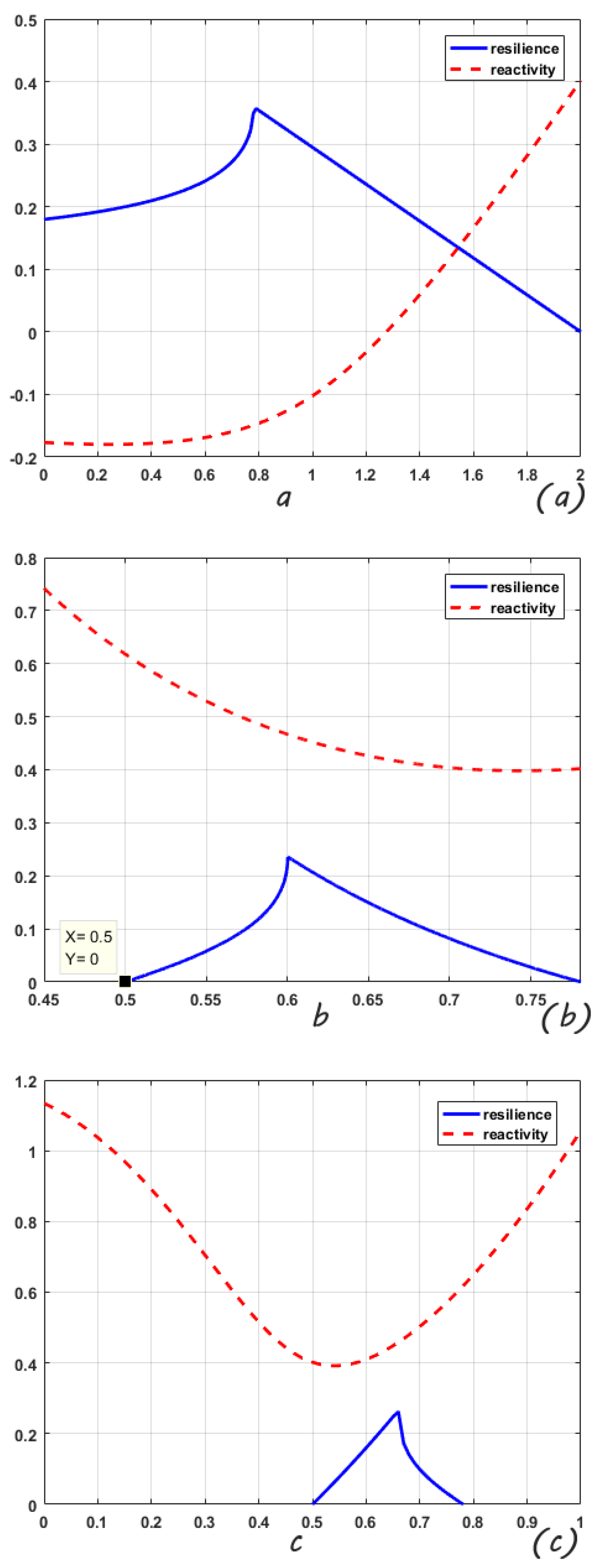
Figure 1 shows the variation of the root-mean-square resilience and root-mean-square reactivity of the studied system within the parameter range when there is no random disturbance. It can be used as a comparison figure for analyzing the influence of random environmental fluctuations on the system. In Figure 1, the parameter ranges of the mean-square stable stage for this system are $a\in [0,2],b\in [0.5,0.7808],c=[0.5,0.7808]$, respectively. Resilience shows a trend of monotonous increase first and then decrease. If b and c are changing parameters, the interior equilibria of the system are both reactive (reactivity $>0$).

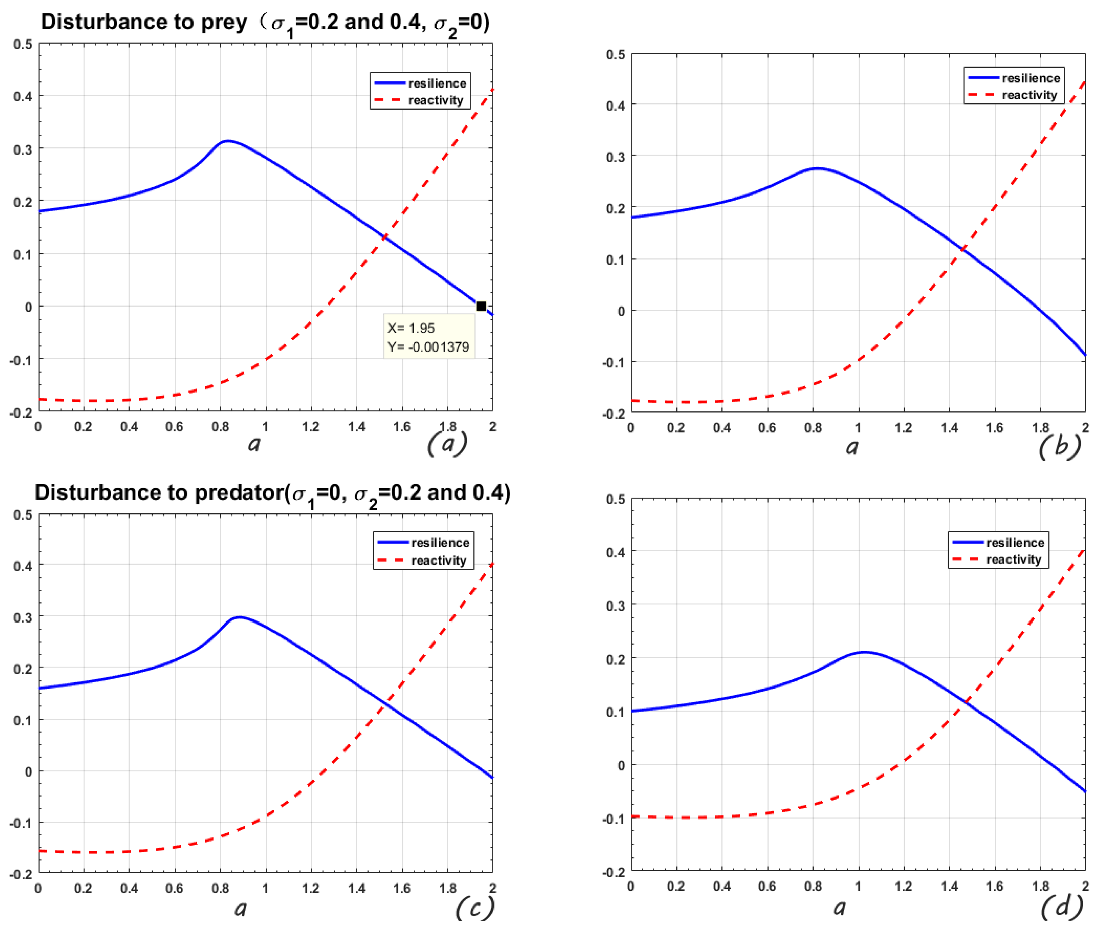
The first column of Figure 2 shows the perturbation only applied to the prey, the disturbance intensity is 0.2 and 0.4, correspondingly. The variable parameter is a. It can be seen that the mean-square stable area of the system is reduced from $a\in [0,2]({\sigma }_1=0,{\sigma }_2=0)$ to $a\in [0,1.96]({\sigma }_1=0.2,{\sigma }_2=0)$ and $a\in [0,1.8]({\sigma }_1=0.4,{\sigma }_2=0)$. The maximum value of resilience (representing the system’s self-recovery ability; the greater the resilience, the more stable the system) is reduced from 0.357 to 0.313 and 0.275. The second column is the disturbance to predator and, similarly, the mean-square stable area is reduced from $a\in [0,2]({\sigma }_1=0,{\sigma }_2=0)$ to $a\in [0,1.96]({\sigma }_1=0,{\sigma }_2=0.2)$ and $a\in [0,1.85]({\sigma }_1=0,{\sigma }_2=0.4)$. The maximum value of resilience is reduced from 0.357 to 0.298 and 0.210. Regarding the reactivity, there is no obvious change when the disturbance is applied to the prey, but when it acts on the predator, the initial value of the reactivity becomes larger as the intensity of the disturbance increases. Summarizing the above conclusions, the system is more sensitive to predator disturbance and reacts more strongly.

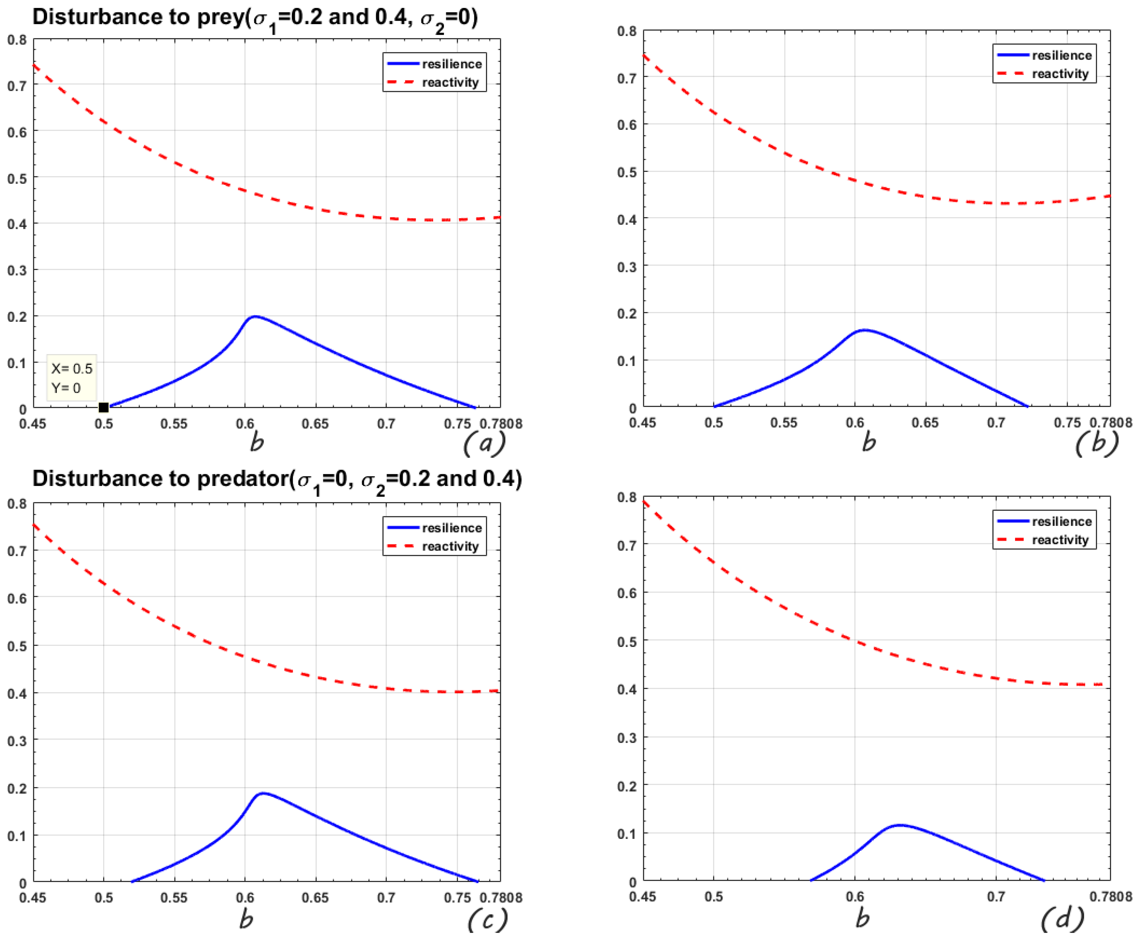
In Figure 3, the range of the change parameter b is $[0,0.7808]$. When the perturbation is only on the prey, the mean-square stable regions of the system are $b\in [0.5,0.763]({\sigma }_1=0.2,{\sigma }_2=0)$ and $b\in [0.5,0.722]({\sigma }_1=0.4,{\sigma }_2=0)$, respectively. The maximum values of resilience are 0.198 and 0.163. When $b\in [0.519,0.765]({\sigma }_1=0,{\sigma }_2=0.2)$ and $b\in [0.568,0.734]({\sigma }_1=0,{\sigma }_2=0.4)$, the model is mean-square stable if the predator is disturbed. Comparing the four sub-figures in Figure 3, it is found that increasing the intensity of the disturbance increases the reactivity, the resilience decreases and the mean-square stable area shrinks. Similar to Figure 2, it is still the predator disturbance that has a stronger impact on the system.

Table 1. Information summary of Figure 4.

Disturbance Intensity	Parameter Value Range of Mean Square Stable Stage	Maximum Value of Resilience
${\sigma }_1=0.2,{\sigma }_2=0$	$d\in [0.52,0.78]$	0.226
${\sigma }_1=0.4,{\sigma }_2=0$	$d\in [0.51,0.76]$	0.213
${\sigma }_1=0,{\sigma }_2=0.2$	$d\in [0.54,0.78]$	0.190
${\sigma }_1=0,{\sigma }_2=0.4$	$d\in [0.53,0.70]$	0.142

is a brief description of Figure 4.

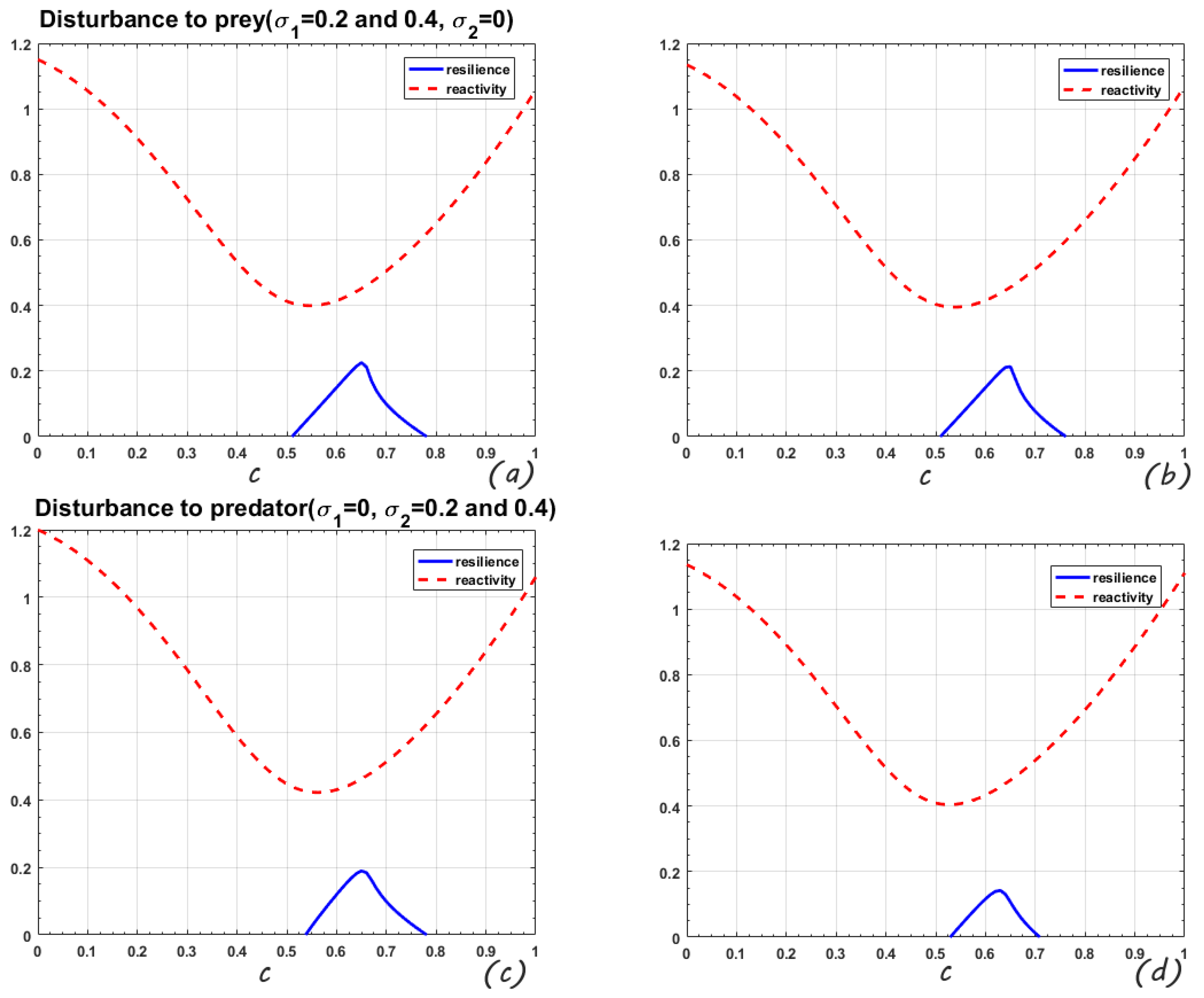
The trends of resilience and reactivity are opposite, which also shows that the more stable the system, the stronger the resilience; the more sensitive the system, the stronger the reactivity.

Compare Figure 2, Figure 3 and Figure 4 with Figure 1, we obtain some conclusions as follows:

• Increasing the random perturbation to any species (predator or prey) will reduce the range of variable parameters of the system in the mean-square asymptotical stable state (where the values of root-mean-square resilience are positive).
• In Figure 2, Figure 3 and Figure 4, we can clearly see that when perturbation is added to any population, the maximum root-mean-square resilience is visibly reduced. In contrast, when the random perturbation is increased for any species, the value of root-mean-square reactivity increases but the increase is not obvious.
• The same random disturbance intensity acts on predator and prey, respectively, the system will be more strongly affected when the predator is disturbed.

4.2. Root-Mean-Square Amplification Envelope (Hopf-Bifurcating Periodic Solution)

Figure 5 shows the root-mean-square amplification envelope of the positive equilibrium of (11) with $a=2.0,b=0.7808,c=0.5$. The positive equilibrium is a stable Hopf-bifurcating periodic solution. Figure 5 illustrates the type of this solution because the change of disturbance is also periodic.

It can be found that adding perturbation to any population at the Hopf-bifurcating equilibrium (even if the perturbation is small) will make the system unstable. In comparison, perturbation to the predator makes the system more sensitive.

Conclusions can be drawn from all the above analyses, and some appropriate suggestions can be made to managers for this ecosystem. For example, when regulating the ecosystem, pay attention to controlling the parameters in the mean-square asymptotically stable state of system (the value of the root-mean-square resilience is positive). Second, according to the numerical graph of root-mean-square amplification envelope, managers can clearly know the maximum value of disturbance magnification: ${\rho }_{max}$ and the time when the maximum disturbance appears: $t_{max}$. If the manager sets a small disturbance to the ecosystem, it needs to consider that the perturbation amplification ${\rho }_{max}$ should be controlled within the range that the system can bear, that is, the system will be mean-square asymptotically stable. $t_{max}$ gives critical information, and decision makers should give orders and actively implement them before $t_{max}$, so as to avoid crucial losses and save money and manpower.

In order to make the reader better understand the significance of root-mean-square amplification envelope, the following numerical example is listed.

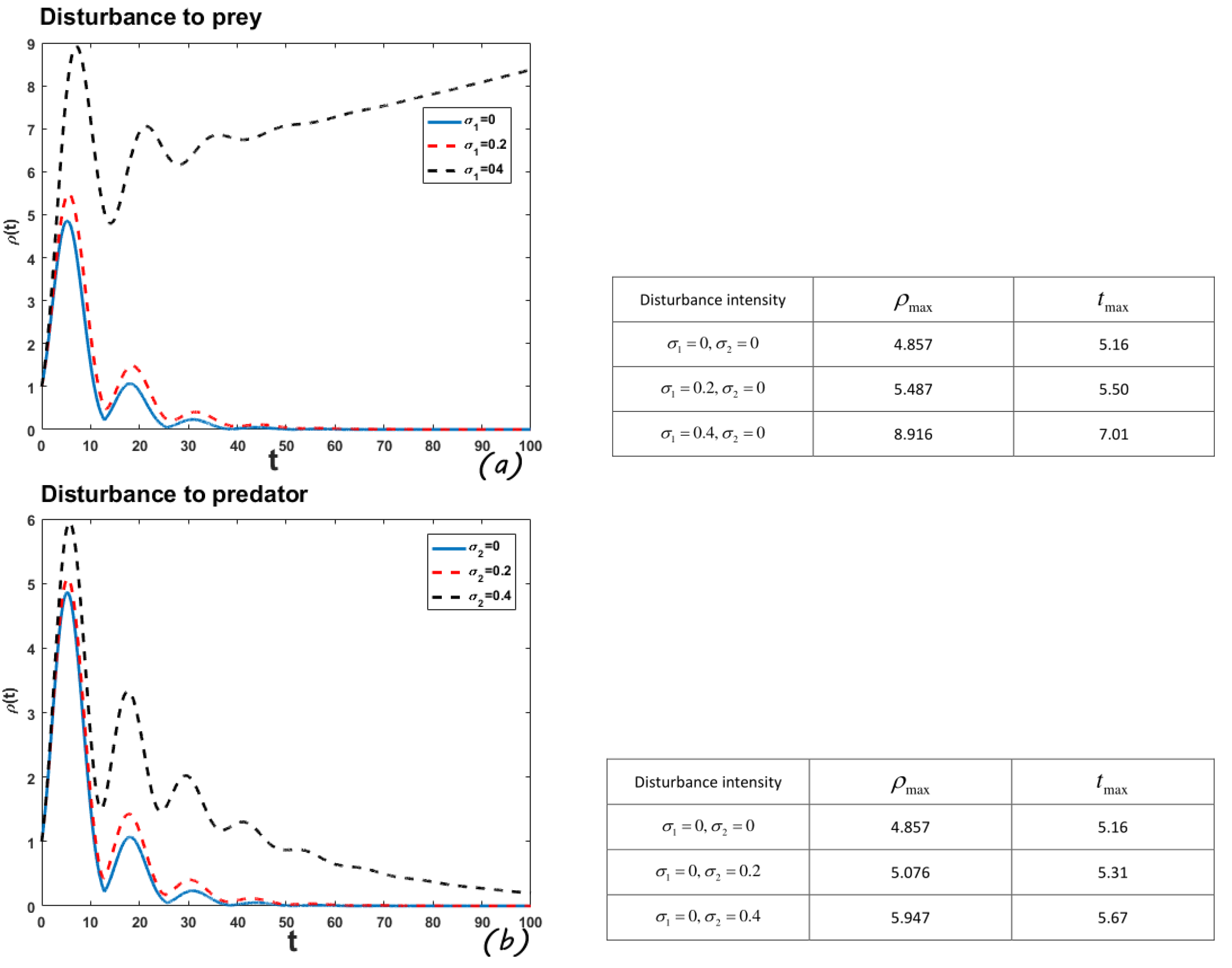
4.3. Root-Mean-Square Amplification Envelope (Locally Stable Positive Equilibrium)

In this example, select the parameter values $a=1.8,b=0.7808,c=0.5$. According to literature [13], the interior equilibrium is locally stable in this case. From Figure 6, we find that when the predator is perturbed, and the perturbation intensity reaches 0.4, the system can still restore a stable state through its own regulation. However, the perturbation can no longer disappear and even shows a constant increasing trend when the prey is perturbed with the perturbation intensity 0.4. At the same time, we can see that no matter which species is disturbed, the greater the perturbation intensity, the larger the amplification envelope.

5. Conclusions

By comparing the root-mean-square resilience and root-mean-square reactivity figures of the stochastic model under different disturbance intensities, we reach the following conclusions: As the perturbation intensity increases, the root-mean-square resilience decreases and, on the contrary, the root-mean-square reactivity increases. As a result, the mean square stability area of the random system reduces, and the mean square stability becomes weaker. In addition, numerical results show that the system is more sensitive when the predator is disturbed. Observing and comparing the figures of the root-mean-square envelope amplification, the following points are found: (1) Adding a disturbance to the Hopf-bifurcation stable periodic solution of the deterministic system, no matter how small the disturbance is, the stability of the solution will be destroyed. (2) The greater the disturbance intensity, the greater the root-mean-square envelope amplification. (3) Applying perturbation to the locally stable positive solution, when the perturbation intensity is small enough, the solution will return to the initial state. However, if the perturbation exceeds critical value, the system will be destroyed and the solution cannot be restored.