Transient Behavior of the MAP/M/1/N Queuing System

Abstract

This paper investigates the characteristics of the MAP/M/1/N queuing system in the transient mode. The matrix method for solving the Kolmogorov equations is proposed. This method makes it possible, in general, to obtain the main characteristics of the considered queuing system in a non-stationary mode: the probability of losses, the time of the transient mode, the throughput, and the number of customers in the system at time t. The developed method is illustrated by numerical calculations of the characteristics of the $MAP/M/1/3$ system in the transient mode.

1. Introduction

Queuing theory is used for the mathematical descriptions of a large number of problems in calculating the performance characteristics of telecommunications and distributed computing systems. As a rule, researchers are interested in the behavior of the system under consideration in a stationary mode, when the probabilities of the states of the system do not depend on time [1,2,3]. However, with the transition to high-speed optical information processing systems and 5G/6G communication systems, for a more accurate assessment of the characteristics of the system, it is necessary to take into account its behavior in a non-stationary mode. Such a mode of operation occurs, for example, when the switching equipment is rebooted, when the base station is turned on and off, when the equipment is switched from the main channel to the backup channel, in cases of equipment malfunction, and in other cases associated with changes in system states. In this case, one of the most important tasks is to determine the duration of the transient mode, that is, the time during which the system will go to a stationary state. This problem is also relevant in the simulation of queuing systems, when it is necessary to determine the moment of transition of the system to a stationary mode with a sufficiently high accuracy.

The transient operation mode of queuing systems was first studied in [4,5,6,7]. In [6], the author for the first time described the need to study the transient operation modes of telecommunication systems and introduced the concept of the time constant of the transient process as an important parameter for determining the rate of transition of the system to the stochastic equilibrium mode. He considered several examples that require taking into account the changes in the probabilities of system states from time to time. As an example, the problem of predicting the characteristics of the system when installing the system or disrupting its operation was presented.

In recent years, queuing systems with periodically varying parameters of input flows and service time for customers have been actively studied [8,9]. One paper [8] considered the problem of convergence for a nonstationary two-processor system with catastrophes, server failures, and repairs, when all parameters are harmonic functions of time. Another paper [9] proposed three different analytical methods for calculating upper bounds for the rate of convergence to a stationary mode of a process given by a continuous inhomogeneous Markov chain. The first method is based on the logarithmic norm of a linear operator function, the second uses the simplest Lyapunov functions, and the third uses differential inequalities. Note that the stability of processes described by Markov chains with periodic parameters was studied back in the 1980s [10,11].

Reference [12] presents an approximate approach to the analysis of the transient behavior of a $M/M/1/N$ system. The time dependencies of the probabilities of the system states are presented for special cases only in numerical calculations. The papers [13,14] present analytical expressions for finding the dependencies of state probabilities on time for the $M/M/1$ queuing system. The solution to the Kolmogorov system of differential equations is sought using the Laplace transform. The papers [15,16] present an analysis of the transient mode of a single-line queuing system with catastrophes. Analytical expressions are given for finding the dependencies of the probabilities of the states of the systems under consideration on time, and their stationary values. The paper [17] investigates a transient operation mode of a queuing system with heterogeneous servers and impatient customers with a Poisson input stream. The most complete review concerning the study of the transient behavior of queuing systems with Poisson input flows is presented in [18]. In this paper, the queuing systems $M/M/\infty$, $M/M/1$, $M/E/1$, and $M/M/1/N$ with catastrophes are investigated.

Despite the described approaches to the analysis of the non-stationary modes of queuing systems with Poisson input flows, these results cannot be used in the design of various real telecommunication systems. This is due to the fact that the traffic of modern telecommunication systems is correlated, and for a more accurate description, one should use not the simplest flow, but Markov correlated MAP or BMAP streams. The monograph [1] presents a systematized presentation of research methods and estimations of stationary characteristics of queuing systems with correlated flows. However, non-stationary modes of queuing systems with MAP flows are poorly studied in the literature. Note, for example, the work [19], which considers a single-line queuing system with correlated input flows, for which a numerical calculation of the state probabilities versus time using the Runge–Kutta method is presented.

This paper, for the first time, proposes an analytical method for studying the transient behavior of the $MAP/M/1/N$ system. The paper is structured as follows. Section 2 gives the formulation of the considered problem of studying the unsteady modes of the $MAP/M/1/N$ system. Section 3 presents an analytical method describing the behavior of the $MAP/M/1/N$ system in a non-stationary mode. Section 4, for the first time, gives expressions for the main parameters of the system under consideration in the transient mode: the probability of losses, the probabilities of the system states, the time of the transient mode, the throughput, and the number of customers in the system at time t. Section 5 presents numerical calculations illustrating the proposed analytical approach for the $MAP/M/1/3$ system.

2. Statement of the Problem

This paper discusses an $MAP/M/1/N$ queuing system with a Markov input flow of customers and a limited number of waiting places. The arrival of customers is controlled by an irreducible non-periodic Markov chain ${\nu }_t,t\ge 0$ with continuous time and a state space $0,1,\dots ,M-1$. The residence time of the chain ${\nu }_t,t\ge 0$ in a certain state $\nu$ has an exponential distribution with the parameter ${\lambda }_{\nu },\nu =\overline{0,M-1}$. After the time spent by the process in this state has expired, with the probability $p^{(1}(\nu ,{\nu }^{\prime })$ the process ${\nu }_t,t\ge 0$ goes to some state ${\nu }^{\prime }$ and a customer is generated, with the probability $p^{\left(0\right)}(\nu ,{\nu }^{\prime })$ that the process makes a transition, but without generating a customer. It is assumed that a jump from the state $\nu$ to the same state is impossible without generating a customer, i.e., $p^{\left(0\right)}(\nu ,\nu )=0$. It is also assumed that the probabilities $p^{\left(k\right)}(\nu ,{\nu }^{\prime }),k=\overline{0,1}$ satisfy the normalization condition

$$\sum _{\begin{array}{c}{\nu }^{\prime }=0\\ {\nu }^{\prime }\ne \nu \end{array}}^{M-1}{p}^{\left(0\right)}(\nu ,{\nu }^{\prime })+\sum _{{\nu }^{\prime }=0}^{M-1}{p}^{\left(1\right)}(\nu ,{\nu }^{\prime })=1,\nu =\overline{0,M-1}$$

(1)

The flow is described by two nonzero $M\times M$-matrices ${\mathbf{D}}_0$ and ${\mathbf{D}}_1$:

$${\mathbf{D}}_0=\left(\begin{array}{cccc}-{\lambda }_0& {\lambda }_0{p}_{0,1}^{\left(0\right)}& ...& {\lambda }_0{p}_{0,M-1}^{\left(0\right)}\\ {\lambda }_1{p}_{1,0}^{\left(0\right)}& -{\lambda }_1& ...& {\lambda }_1{p}_{1,M-1}^{\left(0\right)}\\ ...& ...& ...& ...\\ {\lambda }_{M-1}{p}_{M-1,0}^{\left(0\right)}& {\lambda }_{M-1}{p}_{M-1,1}^{\left(0\right)}& ...& -{\lambda }_{M-1}\end{array}\right)$$

(2)

$${\mathbf{D}}_1=\left(\begin{array}{cccc}{\lambda }_0{p}_{0,0}^{\left(1\right)}& {\lambda }_0{p}_{0,1}^{\left(1\right)}& ...& {\lambda }_0{p}_{0,M-1}^{\left(1\right)}\\ {\lambda }_1{p}_{1,0}^{\left(1\right)}& {\lambda }_1{p}_{1,1}^{\left(1\right)}& ...& {\lambda }_1{p}_{1,M-1}^{\left(1\right)}\\ ...& ...& ...& ...\\ {\lambda }_{M-1}{p}_{M-1,0}^{\left(1\right)}& {\lambda }_{M-1}{p}_{M-1,1}^{\left(1\right)}& ...& {\lambda }_{M-1}{p}_{M-1,M-1}^{\left(1\right)}\end{array}\right)$$

(3)

The monograph [1] describes in detail the meanings of the elements of the matrices ${\mathbf{D}}_0$ and ${\mathbf{D}}_1$. The service time of a customer in the system is exponentially distributed with the parameter $\mu$.

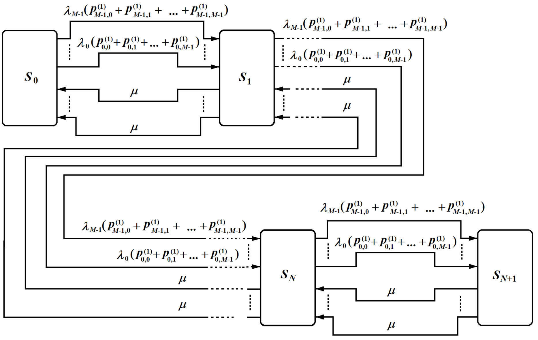
The transition graph of the $MAP/M/1/N$ system is shown in Figure 1. According to this graph, the queuing system $MAP/M/1/N$ can be in one of $K=M(N+2)$ states. The vertices of the graph $S_0$, $S_1$, ..., $S_{N+1}$, designate the macrostates of the buffer and the server. Transitions between these macrostates are accompanied either by the generation of a new customer, or by servicing the old one. Thus, the system is in the $S_0$ macro state if there are no customers in it; that is, the server is idle and the buffer is empty. The system is in the $S_1$ macro state if the server processes one customer and the buffer is empty. The system is in the $S_N$ macrostate, if the server processes one customer, while there are $N-1$ more customers in the buffer. The system is in the $S_{N+1}$ macrostate if the server is busy, provided that there are N customers in the buffer, and the next incoming customer will be discarded. Each of the above macrostates $S_k$, $k=\overline{0,N+1}$ corresponds to M additional states $S_k^{\left(0\right)}$ ...$S_k^{(M-1)}$ of the $MAP$ flow control process without generating a customer. A change in the state of the system $S_k^{\left(0\right)}$ ... $S_k^{(M-1)}$ can occur as a result of one of the $M-1$ state transitions of the control process. Section 5 shows the relationships between the states of the system $S_k^{\left(0\right)}$ ... $S_k^{(M-1)}$ for the case $M=3$. Note that transitions within macrostates $S_k$, $k=\overline{0,N+1}$ correspond to the transitions of the $MAP$ with no customer arrivals, and these transitions are not shown in the generalized graph (Figure 1). Additionally, the transitions between macrostates correspond to transitions of the $MAP$ with customer arrival (M possible transitions) or the service completion with rate $\mu$ (also M possible transitions between states). It is easy to see that the resulting intensity of direct transitions between macrostates is defined as ${\lambda }_g={\sum }_{i=0}^{M-1}{\lambda }_i{\sum }_{j=0}^{M-1}{p}_{ij}^{\left(1\right)}$. In Figure 1, they are specified separately for each intensity ${\lambda }_i$: ${\lambda }_{gi}={\lambda }_i{\sum }_{j=0}^{M-1}{p}_{ij}^{\left(1\right)}$. Reverse transitions between macrostates in the $MAP/M/1/N$ system are determined both by the number of Markov flows M and by the service intensity $\mu$ : ${\mu }_g=(M-1)\mu$ (see Figure 1).

Following [1], the Kolmogorov equation system for the $MAP/M/1/N$ system under consideration can be written as

$$\frac{d}{dt}\overrightarrow{P}=\mathbf{A}\overrightarrow{P}$$

(4)

in the matrix form where

$$\mathbf{A}=\left(\begin{array}{ccccc}{\mathbf{D}}_0^T& \mu \mathbf{I}& ...& O& O\\ {\mathbf{D}}_1^T& {\mathbf{D}}_0^T-\mu \mathbf{I}& ...& O& O\\ ...& ...& ...& ...& ...\\ O& O& ...& \mu I& O\\ O& O& ...& {\mathbf{D}}_0^T-\mu I& \mu I\\ O& O& ...& {\mathbf{D}}_1^T& {\mathbf{D}}_0^T+{\mathbf{D}}_1^T-\mu \mathbf{I}\end{array}\right)$$

(5)

$\overrightarrow{P}\left(t\right)={\left({\overrightarrow{P}}_0,{\overrightarrow{P}}_1,\cdots ,{\overrightarrow{P}}_{N+1}\left(t\right)\right)}^T$; T is a transposition operator; ${\overrightarrow{P}}_k,k=\overline{0,N+1}$ is the macrostate $S_k$ probability column vector (the M states of $S_k^{\left(0\right)}$ ... $S_k^{(M-1)}$) of the server and buffer, determined by the dimension of the matrices (2) and (3). Note that ${\mathbf{A}}^T$ is an infinitesimal generator and ${\mathbf{A}}^T\overrightarrow{e}=\overrightarrow{0}$. Here $\overrightarrow{e}$ is the unit column; $\overrightarrow{0}$ is the zero column.

The purpose of this work is an analytical study of the transient mode of the system under consideration. We propose a new approach for analyzing the transient mode of the $MAP/M/1/N$ queuing system and finding analytical expressions for the probability of losses, transient time, throughput, and the number of customers in the system at the time t. The advantages of the proposed approach are the simplification of numerical calculations and the possibility of solving further problems of the synthesis of the corresponding systems.

3. The Method of Studying the Non-Stationary Characteristics of the MAP/M/1/N System

First of all, we need to formulate the main theoretical provisions necessary for studying the non-stationary mode of the $MAP/M/1/N$ queuing system.

3.1. Analysis of the Characteristic Polynomial Roots

This subsection analyzes the roots of the characteristic polynomial of the Kolmogorov equations (4) (the eigenvalues of the coefficient matrix (5)), which describe the $MAP/M/1/N$ system. This analysis is of great importance for describing the behavior of this system in a transient mode, since these roots determine the duration of the transient mode and the kind of the dependence of the state probabilities on time. According to [20,21,22], the characteristic polynomial of the Kolmogorov system (4) of order K has the form

$${\gamma }^K+b_{K-1}{\gamma }^{K-1}+...+b_2{\gamma }^2+b_1\gamma +b_0=0$$

(6)

Here $b_j$ are the coefficients expressed in terms of the elements of the matrix (5) [20,21,22,23,24], and $\gamma$ are the roots of the characteristic polynomial of system (4).

Since the probabilities in (4) are linearly dependent, and accordingly, $({\mathbf{D}}_0+{\mathbf{D}}_1)\overrightarrow{e}=\overrightarrow{0}$ [1], the determinant of the coefficient matrix (5) is equal to zero [24]. Taking into account the well-known equality $b_0=det\mathbf{A}$ [24], it can be obtained from (6) that

$$\gamma (b_{K-1}{\gamma }^{K-1}+...+b_2{\gamma }^2+b_1\gamma )=0.$$

(7)

Thus, one of the roots ${\gamma }_0$ of the characteristic Equation (6) is necessarily equal to zero. Since matrix (5) is real, the roots of characteristic Equation (6) can be either real or complex conjugate [24].

In addition, based on Sylvester’s theorem [25,26,27], the number of negative diagonal elements of matrix (5) is equal to the number of negative eigenvalues of this matrix. Since all diagonal elements (5), taking into account (2) and (3), are negative, all roots of the characteristic equation have negative real parts.

Thus, the roots of the characteristic polynomial of the Kolmogorov system of differential equations describing the behavior of the $MAP/M/1/N$ system can be either real negative or pairwise complex conjugate with negative real parts.

Consequently, the transient mode in the $MAP/M/1/N$ system always has a decaying exponential character (Figure 2a), if the characteristic numbers are real negative or of decaying wavy character [20,21,22] (Figure 2b), if at least two eigenvalues are complex conjugates with negative real parts.

In accordance with [20,21,22,23,24], the roots of the characteristic equation (Equation (4)) can be either simple or multiple. This study, for the sake of definiteness, considers only the case of simple roots, which is most often encountered in practice.

3.2. The Matrix Method for Solving the Kolmogorov Equations

The papers [4,5,6,7,8,9,10,11,12,13,14,15,16,17,18] present various methods of studying the non-stationary mode of queuing systems. All of them are reduced either to a numerical solution of the corresponding Kolmogorov system, or to the use of Laplace transforms. All of them do not allow obtaining a general solution to the Kolmogorov system of equations.

This paper presents the analytical approach based on the use of the so-called probability translation matrix.

Definition 1.

The probability translation matrix $\mathit{L}\left(t\right)$ of system states is the matrix that relates the state probabilities $P\left(t\right)$ at an arbitrary moment of time t with the probabilities of the states $P\left(t_0\right)$ of this system at the initial moment of time $t_0$:

$$\overrightarrow{P}\left(t\right)=\mathbf{L}\left(t\right)\overrightarrow{P}\left(t_0\right)$$

(8)

Obviously, the dimension K of the matrix $\mathbf{L}$ in (8) is equal to the order of system (4). However, the rank of this matrix is less by one than the order of system (4), since the probability of one of the states is expressed in terms of the remaining probabilities. Note that in this case, it is not necessary to fulfill the condition $t_0=0$. In this case, the initial moment of time is understood as the moment of the beginning of observation over the behavior of a random process.

Theorem 1.

The state probability of the queuing system MAP/M/1/N with constant parameters ${\lambda }_i$, $p_{kl}^{\left(j\right)}$, $i,k,l=\overline{0,M-1}$, $j=\overline{0,1}$, μ in the transient mode is fully described by the translation matrix at any time moment t, if the initial values of the state probabilities of the given system $\overrightarrow{P}\left(t_0\right)$ are known.

Proof. 

First of all, it should be noted that system (4) is overdetermined under the condition that there exists a stationary state; therefore, the rank of the fundamental matrix is less by one than the dimensions of the coefficient matrix of the system (4), and one of the solutions of the Kolmogorov system is a linear combination of the others. Additionally, solutions to system (4) can be written in the form

$$\overrightarrow{P}\left(t\right)=\mathbf{Y}\left(t\right)\overrightarrow{C}$$

(9)

where

$$\mathbf{Y}\left(t\right)=\left(\begin{array}{cccc}{\xi }_{00}exp\left({\gamma }_{0}t\right)& {\xi }_{01}exp\left({\gamma }_{1}t\right)& ...& {\xi }_{0,K-1}exp\left({\gamma }_{K-1}t\right)\\ {\xi }_{10}exp\left({\gamma }_{0}t\right)& {\xi }_{11}exp\left({\gamma }_{1}t\right)& ...& {\xi }_{1,K-1}exp\left({\gamma }_{K-1}t\right)\\ ...& ...& ...& ...\\ {\xi }_{K-1,0}exp\left({\gamma }_{0}t\right)& {\xi }_{K-1,1}exp\left({\gamma }_{1}t\right)& ...& {\xi }_{K-1,K-1}exp\left({\gamma }_{K-1}t\right)\end{array}\right)$$

(10)

${\xi }_{kl}$ are the elements of the eigen-basis of the coefficient matrix of system (4) (the coefficients relating the probabilities of states); $\overrightarrow{C}$ is the column of integration constants determined by the initial conditions. Then for $t=t_0$:

$$\overrightarrow{P}\left(t_0\right)=\mathbf{Y}\left(t_0\right)\overrightarrow{C}$$

(11)

From (11) we have

$$\overrightarrow{C}={\mathbf{Y}}^{-1}\left(t_0\right)\overrightarrow{P}\left(t_0\right)$$

(12)

Substituting (12) into (9), one can obtain

$$\overrightarrow{P}\left(t\right)=\mathbf{Y}\left(t\right){\mathbf{Y}}^{-1}\left(t_0\right)\overrightarrow{P}\left(t_0\right)$$

(13)

or

$$\overrightarrow{P}\left(t\right)=\mathbf{L}\left(t\right)\overrightarrow{P}\left(t_0\right)$$

(14)

where

$$\mathbf{L}\left(t\right)=\mathbf{Y}\left(t\right){\mathbf{Y}}^{-1}\left(t_0\right)$$

(15)

is the translation matrix. Thus, it follows from (14) that the matrix $\mathbf{L}\left(t\right)$ relates the states of the process at the time t with these states at the time $t_0$. Moreover, if $\mathbf{Y}\left(t_0\right)=\mathbf{I}$, where $\mathbf{I}$ is the unit diagonal matrix, then $\mathbf{L}\left(t\right)=\mathbf{Y}\left(t\right)$. □

Obviously, the matrix (15) is neither a Cauchy matrix nor a fundamental matrix [22], since the system (4) is overdetermined, and the rank of these matrices is less by one than the dimensions of the matrix (15). Moreover, as $t\to \infty$, determinant (15) tends to zero; and the determinant of the fundamental matrix is the Wronski determinant and is never equal to zero [24].

An important advantage of the presented approach is a decrease in the computational complexity associated with transformations that exclude the linear dependence of solutions when using fundamental matrices and calculating the Jordan forms of matrices. Moreover, this approach does not require the use of Laplace transforms and allows one to effectively solve synthesis problems (the so-called inverse problems).

Now it is important to find the general analytical form of the solution for the queuing system under consideration. In the most general case, this solution is found as an exponent of the coefficient matrix of the initial differential equation [24]. However, the calculation of the matrix exponent requires finding the Jordan form of the original matrix and the matrix of eigenvectors, which for large sizes of the system is a very cumbersome operation and gives large errors. Moreover, this approach does not allow writing the final expression in an analytical form. This paper proposes the technique for finding this solution based on Theorem 1 without using the procedure for calculating the matrix exponent.

Theorem 2.

The translation matrix of the probabilities of the queuing system $MAP/M/1/N$ with constant parameters ${\lambda }_i$, $p_{kl}^{\left(j\right)}$, $i,k,l=\overline{0,M-1}$, $j=\overline{0,1}$, μ; and simple roots of the characteristic polynomial (7), has the form

$$\mathbf{L}=\sum _{j=0}^{K-1}{\mathbf{A}}_{j}exp\left({\gamma }_{j}t\right)$$

(16)

where the elements of the $K\times K$ matrix ${\mathbf{A}}_j$ are written as

$${\left(A_j\right)}_{kl}={(-1)}^{k+l}\frac{{\Delta }_{lj}}{\Delta }{\xi }_{kj}$$

(17)

$$\Delta =det\left(\begin{array}{cccc}{\xi }_{00}& {\xi }_{01}& \dots & {\xi }_{0,K-1}\\ {\xi }_{10}& {\xi }_{11}& \dots & {\xi }_{1,K-1}\\ ⋮& ⋮& \ddots & ⋮\\ {\xi }_{K-1,0}& {\xi }_{K-1,1}& \dots & {\xi }_{K-1,K-1}\end{array}\right)$$

(18)

${\Delta }_{lj}$ is the determinant of the algebraic complement to the element ${\xi }_{lj}$ of the matrix Δ, Δ is the proper basis of the matrix of coefficients of system (4) in K-dimensional space [22,23,24], and ${\gamma }_j$ is the j-th root of the characteristic polynomial (7) of system (4).

Proof 

(Proof). As noted above, the general solution of the system of linear homogeneous differential equations (4) with constant coefficients and simple roots of the characteristic equation has the form [20,21,22,23,24]

$$P_j\left(t\right)=\sum _{j=0}^{K-1}{\xi }_{ij}{C}_{j}exp\left({\gamma }_{j}t\right),i=\overrightarrow{1,K-1}$$

(19)

One should look for the elements of the transformation matrix under the condition $\mathbf{Y}\left(t_0\right)=\mathbf{I}$ (see (15)). Then the constants $C_j$ for the elements of the first column are found under the condition $P_i\left(t_0\right)={(1,0,\cdots ,0)}^T$; i.e., the system of equations to be solved has the form

$$\begin{array}{c}{\displaystyle \sum _{j=0}^{K-1}{\xi }_{0,j}{C}_{0,j}=1}\\ {\displaystyle \sum _{j=0}^{K-1}{\xi }_{1,j}{C}_{0,j}=0}\\ ⋮\\ {\displaystyle \sum _{j=0}^{K-1}{\xi }_{K-1,j}{C}_{0,j}=0}\end{array}$$

(20)

or in a matrix form

$$\left(\begin{array}{cccc}{\xi }_{0,0}& {\xi }_{0,1}& \dots & {\xi }_{0,K-1}\\ {\xi }_{1,0}& {\xi }_{1,1}& \dots & {\xi }_{1,K-1}\\ ⋮& ⋮& \ddots & ⋮\\ {\xi }_{K-1,0}& {\xi }_{K-1,1}& \dots & {\xi }_{K-1,K-1}\end{array}\right)\left(\begin{array}{c}{C}_{0,0}\\ C_{1,0}\\ ⋮\\ C_{K-1,0}\end{array}\right)=\left(\begin{array}{c}1\\ 0\\ ⋮\\ 0\end{array}\right)$$

(21)

Hence, one can obtain

$$C_{j,0}={(-1)}^{1+j}\frac{{\Delta }_{1,j}}{\Delta }$$

(22)

Substitution of the $C_{j1}$ found in (19) gives the elements

$$L_{i1}=\sum _{j=0}^{K-1}\frac{{\Delta }_{1,j}}{\Delta }\xi ijexp\left({\gamma }_{j}t\right)$$

(23)

of the first column of the transformation matrix. Similarly, the elements of the second column are found under the condition $P_i\left(t_0\right)={(0,1,\cdots ,0)}^T$, as well as the elements of the $K-1$ column under the initial conditions $P_i\left(t_0\right)={(0,0,\cdots ,1)}^T$. □

4. System Characteristics in the Transient Mode

The main indicators of the system in the transient mode are the probability of losses, the time of the transient mode, throughput, and the number of customers in the system [17,18]. As a rule, these indicators for various systems are studied in a stationary mode. The paper [6] presents relations for calculating the so-called time constant of a random process, but provides no substantiation for this parameter, even for the $M/M/1/N$ system. Moreover, there are no ratios for calculating the transient time. The paper [18] considers the problem of the maximum queue size on the interval $[0,t]$, the probability of losses, and the number of customers in the system at time t for the systems $M/M/1$ and $M/M/1/N$. The author used the uniformization procedure, passing from continuous to discrete time, which significantly complicated the calculations. At the same time, the calculation of the throughput of queuing systems in the transient mode has not yet been considered in the world scientific literature known to the authors.

4.1. Loss Probability

The expression discovered for the transformation matrix (16) allows calculating the probability of packet loss at each time instant of the transient mode as the sum of the probabilities of the states $S_{N+1}^{\left(0\right)}...S_{N+1}^{(M-1)}$ in this moment in time [1].

$$P_{loss}=\sum _{i=0}^{M-1}{P}_{N+1}^{\left(i\right)}\left(t\right)$$

(24)

where $P_{N+1}^{\left(i\right)}\left(t\right)$ are the probabilities of states $S_{N+1}^{\left(0\right)}...S_{N+1}^{(M-1)}$ at the time t. Taking into account the form of transformation matrix (16), the probability of losses can be written in the form

$$P_{loss}=\sum _{i=K-M}^{K-1}\sum _{j=0}^{K-1}{L}_{ij}(t-t_0)P_j\left(t_0\right)$$

(25)

where $L_{ij}\left(t\right)$ are elements of matrix (16) at the time t.

4.2. Transient Time

Determining the transient time is one of the most important unsolved problems in the theory of $MAP$ flows. It was indicated above that the values of the characteristic numbers fully described the duration and nature of the transient mode. Now let us consider the duration of the transient mode. In the general case, based on the analysis carried out in Section 3.1, the probability of the i-th state is

$$P_i\left(t\right)={\xi }_{i0}{C}_0+\sum _{j=1}^{K-1}{\xi }_{ij}{C}_{j}exp\left({\gamma }_{j}t\right)$$

(26)

where ${\gamma }_j<0,j=\overline{1,K-1}$. That is, the overall process is a superposition of K-1 damped processes. If all ${\gamma }_j$ except ${\gamma }_0$ are real negative, then at $t\to \infty$, $P_i\left(t\right)\to {\xi }_{i1}{C}_1$. Each of the exponential terms in (26) decreases by a factor of e over some time ${\tau }_j$. This time will here be called the time constant of the j-th component of a random process with an input $MAP$ flow, by analogy with the time constant borrowed by Harison [6] from the theory of electrical circuits for $M/M/n$ queuing systems. However, it should be noted that the physical meaning of this quantity was not described in [6]. This constant can be calculated for real ${\tau }_j$ based on the equality $exp(-|{\gamma }_j\left|{\tau }_j\right)=1⁄e=e^{-1}$, taking into account that ${\gamma }_0=0,\forall {\gamma }_j<0,j=\overline{1,K-1}$, whence, ${\tau }_j=1⁄\left|{\gamma }_j\right|$. In this case, a decrease in ${\gamma }_j$ leads to an increase in ${\tau }_j$. Thus, the term in (26) with the minimum ${\gamma }_j$ has the maximum time for decreasing by a factor of e. It also determines the transient mode duration.

In the case of complex ${\gamma }_j={\alpha }_j+i{\beta }_j$, the corresponding independent solution (4) is in the form $exp\left({\alpha }_{j}t\right)cos\left({\beta }_{j}t\right)$ [20,21,22,23,24], where, based on Theorem 1, ${\alpha }_j<0$. Therefore, the time constant of the j-th component of a random process can be defined as $exp(-|{\alpha }_j\left|{\tau }_j\right)=1/e=e^{-1}$. Thus, the following definition can be formulated.

Definition 2.

The time constant of a random process with an input MAP flow with constant parameters ${\lambda }_i$, $p_{kl}$, μ is the time during which the component of the process with the smallest ${\alpha }_j$ decays by e times. Its value is equal to the inverse smallest real part of the nonzero eigenvalue ${\gamma }_j={\alpha }_j+i{\beta }_j$, $i=\sqrt{-1}$; i.e., ${\tau }_j=1⁄{\alpha }_{jmin}$, where $\forall {\alpha }_j\in \Gamma :(\Gamma ={\alpha }_j,{\alpha }_j\ge {\alpha }_{m}in\Rightarrow {\alpha }_j={\alpha }_{min})$.

Based on the mathematical formulation of the problem, the transient mode ends at $\to \infty$, but from a physical point of view, the time of the transient mode can be considered finite at $|P_j\left(t\right)-{\pi }_j|\le ϵ$, where ϵ is some infinitesimal value, and ${\pi }_j$ is the stationary probability of the j-th state. The choice of ϵ is determined by the practical requirements for specific queuing systems. Now, it will be assumed that the mode can be considered stationary when the value of the j-th term decreases in (26) with ${\gamma }_{(}j)={\alpha }_{jmin}+i{\beta }_j$ in $e^3$. Then, the transient time is defined as ${\tau }_{tr}=3⁄\left|{\alpha }_{jmin}\right|$. Similarly, for the damping of the transient process by $e^5$ times, one can write ${\tau }_{tr}=5⁄\left|{\alpha }_{jmin}\right|$.

Definition 3.

In the general case, the time of the transient process can be defined as ${\tau }_{tr}=k⁄\left|{\alpha }_{jmin}\right|$, where $\forall {\alpha }_j\in \Gamma :(\Gamma ={\alpha }_j,{\alpha }_j\ge {\alpha }_{min}\Rightarrow {\alpha }_j={\alpha }_{min}$. Here $k(k>0,k\in R)$ is defined as the coefficient of change in the state probability.

The numerical simulation presented below has shown that for practical calculations, $k=5÷10$ is sufficient, depending on the formulation of the problem.

When considering the nature of the transient mode, the ratio of ${\alpha }_j$ and ${\beta }_j$ is important. Indeed, if two roots of the characteristic equation are complex conjugate, then one of the terms in the elements of matrix (16) has the form $exp\left(\alpha t\right)cos\left({\beta }_{j}t\right)$. Thus, ${\beta }_j$ determines the oscillation frequency of state probabilities in the transient mode. If ${\beta }_j\gg {\alpha }_j$, then oscillations are practically not observed. If ${\beta }_j<{\alpha }_j$, then one half-period of oscillations can be observed. If ${\beta }_j\approx {\alpha }_j$, then one oscillation period can be observed. If ${\beta }_j\gg {\alpha }_j$, then the process in the transient mode has a wavy character.

4.3. Throughput

The found probability of losses $P_{loss}\left(t\right)$ (25) makes it possible to calculate the throughput of the system at a given time in accordance with the definition [3] as

$$A\left(t\right)=\left(1-P_{loss}\left(t\right)\right)\lambda =\left(1-\sum _{i-0}^{M-1}{P}_{N-1}^{\left(i\right)}t\right)\lambda$$

(27)

Here $\lambda =\theta {\mathbf{D}}_1\overrightarrow{e}$ is the average intensity of the input flow [1]. Taking into account matrix (16):

$$A\left(t\right)=\left(1-\sum _{i=K-M}^{K-1}\sum _{j=0}^{K-1}{L}_{ij}(t-t_0)P_j\left(t_0\right)\right)\lambda ,$$

(28)

the average value of the throughput during the transient process is

$$\begin{array}{c}{\displaystyle A_{mid}=\frac{1}{{\tau }_{tr}}{\int }_{t_0}^{t_0+{\tau }_{tr}}A\left(t\right)dt=}\\ {\displaystyle =\frac{1}{{\tau }_{tr}}{\int }_{t_0}^{t_0+{\tau }_{tr}}\left(1-\sum _{i=K-M}^{K-1}\sum _{j=0}^{K-1}{L}_{ij}(t-t_0)P_j\left(t_0\right)\right)\lambda dt}\end{array}$$

(29)

4.4. The Number of Customers in the System at the Time t

Knowing the probability that the system is idle, that is, both the buffer is empty and the server is idle, one can determine the mathematical expectation of the average number of customers in the system at the time t [17] by the formula:

$$E\left(n\left(t\right)\right)=\sum _{i=1}^{N+1}i\sum _{j=0}^{M-1}{p}_i^{\left(j\right)}\left(t\right)$$

(30)

Indeed, the probability of the system macrostate $S_i$ at the time t is equal to ${\sum }_{j=0}^{M-1}{p}_i^{\left(j\right)}\left(t\right)$ (Section 2). In this case, i customers in the system correspond to the macrostate $S_i$. Then the mathematical expectation in accordance with the definition can be calculated by formula (30). Then the average statistical value of the number of received customers in the system during the transient process is

$$\begin{array}{c}{\displaystyle n_{mid}=\frac{1}{{\tau }_{tr}}{\int }_{t_0}^{t_0+{\tau }_{tr}}E\left(n\left(t\right)\right)dt=}\\ {\displaystyle =\frac{1}{{\tau }_{tr}}{\int }_{t_0}^{t_0+{\tau }_{tr}}\sum _{i=1}^{N+1}i\sum _{j=0}^{M-1}{p}_i^{\left(j\right)}\left(t\right)dt}\end{array}$$

(31)

Obviously, the integral in (31) is calculated analytically, since the integrand is the sum of exponentials. Integral (31) also has an analytical solution. However, the resulting analytical expressions are not given here due to their cumbersomeness.

5. Examples of a Numerical Study of the Characteristics of the MAP/M/1/N System

This section considers the process of servicing three types of traffic with the arrival rates ${\lambda }_0=5$ packets/s, ${\lambda }_1=583$ packets/s, and ${\lambda }_2=833$ packets/s. Assuming that the input flows are correlated, the values of the flow rates can be set by the matrix $\mathbf{\Lambda }=\mathrm{diag}\{{\lambda }_0,{\lambda }_1,{\lambda }_2\}=\mathrm{diag}\{5,583,833\}$. In this problem, transitions from the transmission state of one traffic with intensity ${\lambda }_n$ to the transmission state of another type of traffic with intensity ${\lambda }_m$ without generating customers are given by the transition probability matrix

$${\mathbf{P}}^{\left(0\right)}=\left(\begin{array}{ccc}0& p_{01}^{\left(0\right)}& p_{02}^{\left(0\right)}\\ p_{10}^{\left(0\right)}& 0& p_{12}^{\left(0\right)}\\ p_{20}^{\left(0\right)}& p_{21}^{\left(0\right)}& 0\end{array}\right)=\left(\begin{array}{ccc}0& 0.5& 0.01\\ 0.02& 0& 0.5\\ 0.02& 0.04& 0\end{array}\right)$$

(32)

$${\mathbf{P}}^{\left(1\right)}=\left(\begin{array}{ccc}{p}_{00}^{\left(1\right)}& p_{01}^{\left(1\right)}& p_{02}^{\left(1\right)}\\ p_{10}^{\left(1\right)}& p_{11}^{\left(1\right)}& p_{12}^{\left(1\right)}\\ p_{20}^{\left(1\right)}& p_{21}^{\left(1\right)}& p_{22}^{\left(1\right)}\end{array}\right)=\left(\begin{array}{ccc}0.01& 0.1& 0.38\\ 0.01& 0.1& 0.37\\ 0.01& 0.1& 0.83\end{array}\right)$$

(33)

It is taken into account that a jump from one state to the same state is impossible without generating a customer—i.e., $p_{\nu ,\nu }^{\left(0\right)}=0$; and the probabilities satisfy the normalization condition ${\sum }_{j=0}^2{p}_{ij}^{\left(0\right)}+{\sum }_{j=0}^2{p}_{ij}^{\left(1\right)}=1$, $i=\overline{0,2}$. Thus, the information flow from a multimedia device can be specified as a $MAP$-flow described by two nonzero matrices ${\mathbf{D}}_0=\mathbf{\Lambda }({\mathbf{P}}^{\left(0\right)}-\mathbf{I})$, ${\mathbf{D}}_1=\mathbf{\Lambda }{\mathbf{P}}^{\left(1\right)}$ [1]. It follows from the problem statement that the number of states of the $MAP$ governing process is $M=3$. In addition, it can be assumed that the server is a switch with a buffer size of $N=1$. 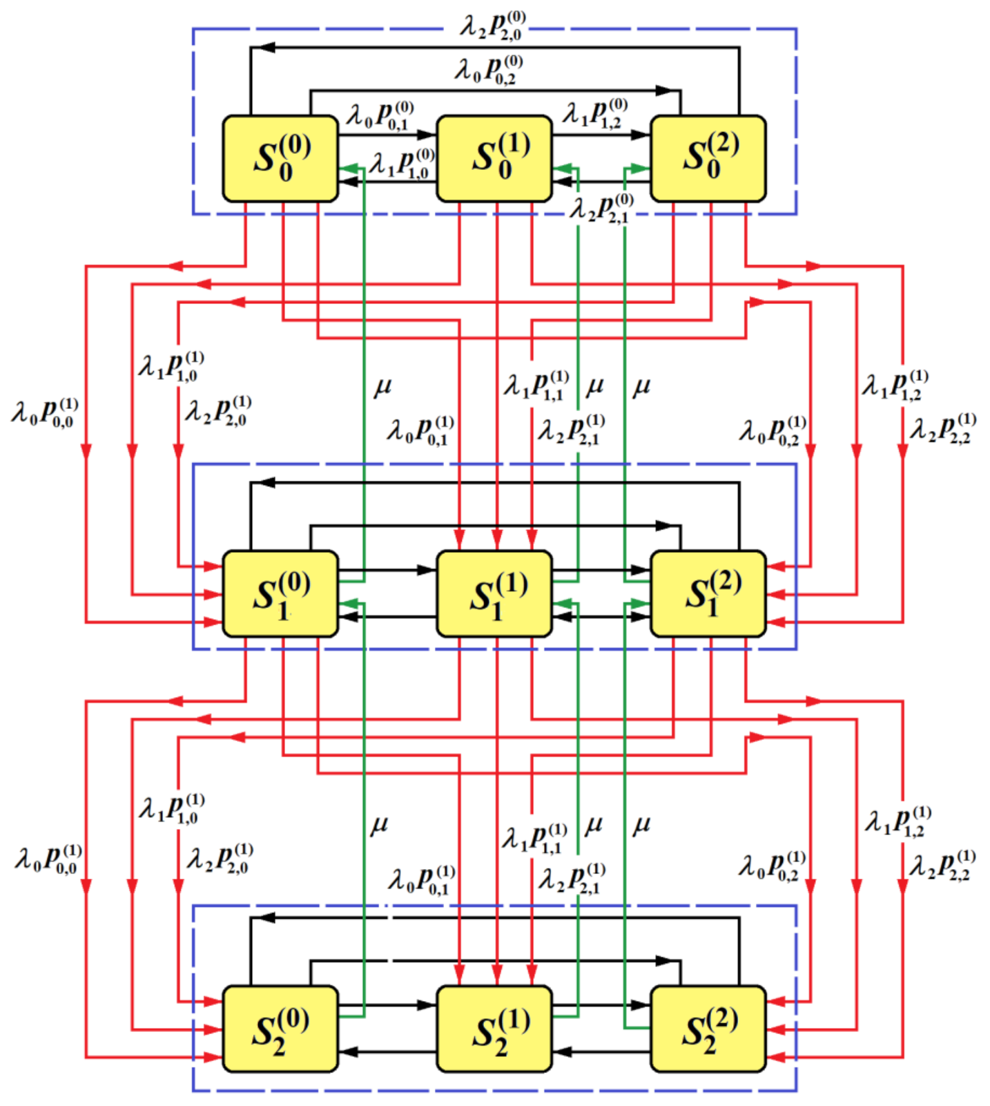The transition graph for the case under consideration is shown in Figure 3. Here the states $S_0^{\left(0\right)}$, $S_0^{\left(1\right)}$, and $S_0^{\left(2\right)}$ correspond to the free states of the server (macrostate ${\mathbf{S}}_0$), and are outlined in blue. The states $S_1^{\left(0\right)}$, $S_1^{\left(1\right)}$, and $S_1^{\left(2\right)}$ correspond to the states of the serving device transmitting one of the traffic types: $S_1^{\left(0\right)}$ voice, $S_1^{\left(1\right)}$ video, or $S_1^{\left(2\right)}$ data (macrostate ${\mathbf{S}}_1$). The states $S_2^{\left(0\right)}$, $S_2^{\left(1\right)}$, and $S_2^{\left(2\right)}$ (or macrostate ${\mathbf{S}}_2$) correspond to the states of the serving device transmitting one of the traffic types—$S_2^{\left(0\right)}$ for voice, $S_2^{\left(1\right)}$ for video, and $S_2^{\left(2\right)}$ for data—but there is already a packet with this type of traffic in the buffer. In view of the above, transitions from one state to another are given by the matrices

$${\mathbf{D}}_0=\left(\begin{array}{ccc}-{\lambda }_0& 0.5{\lambda }_0& 0.01{\lambda }_0\\ 0.02{\lambda }_1& -{\lambda }_1& 0.5{\lambda }_1\\ 0.02{\lambda }_2& 0.04{\lambda }_2& -{\lambda }_2\end{array}\right)$$

(34)

$${\mathbf{D}}_1=\left(\begin{array}{ccc}0.01{\lambda }_0& 0.1{\lambda }_0& 0.38{\lambda }_0\\ 0.01{\lambda }_1& 0.1{\lambda }_1& 0.37{\lambda }_1\\ 0.01{\lambda }_2& 0.1{\lambda }_2& 0.83{\lambda }_2\end{array}\right)$$

(35)

For the research, a software package in the Python language was developed.

Let us investigate the dependence of the state probabilities on the ratio of the intensities of packet arrival and traffic service. To do this, consider the following three cases for all real ${\gamma }_k$:

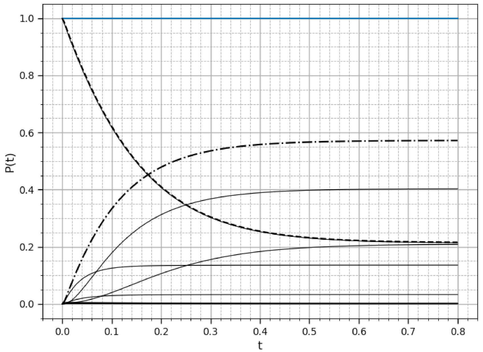
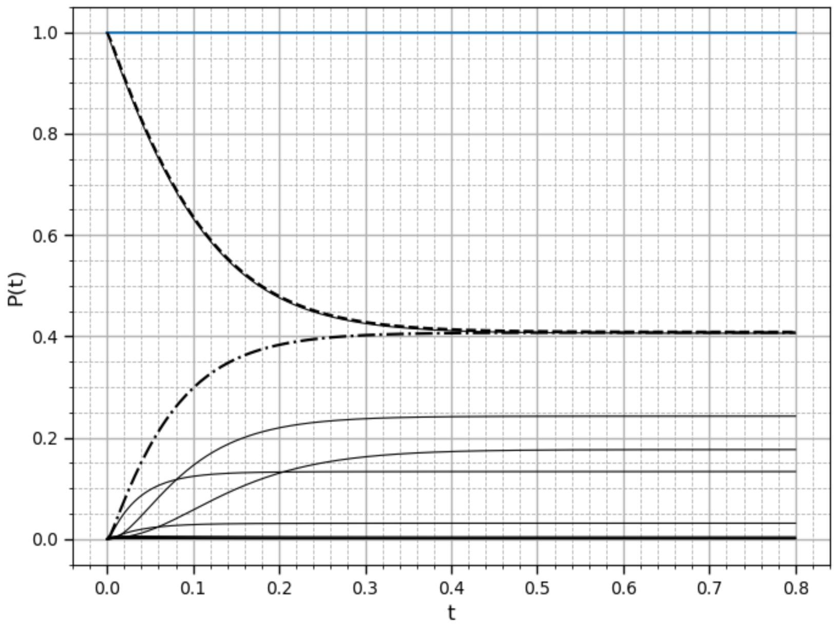
(1) The average service rate $\mu =5$ packets/s; the average rate of packet arrival in accordance with [1] $\lambda =139.04$ packets/s. According to the results of the calculation, the minimum characteristic indicator in modulus is ${\gamma }_{min}=-8.9145$. The results of calculating the state probabilities are presented in Figure 4. Solid lines indicate the probabilities of system states. The probability of losses for this case is indicated by a dashed and dotted line, which, during the transient mode, increases from zero at $t=0$ s to $0.57$ at $t>0.56$ s. The time dependence of the probability of a free state of the system is indicated by a dashed line and varies from unity at $t=0$ s to $0.21$ at $t>0.56$ s. The time constant for this case, in accordance with Definition 2, is ${\tau }_{max}=1⁄\left|{\gamma }_{min}\right|=1⁄8.9145=0.112$ s, and the transient time ${\tau }_{t}r=0.56$ s for $k=5$ in accordance with Definition 3.

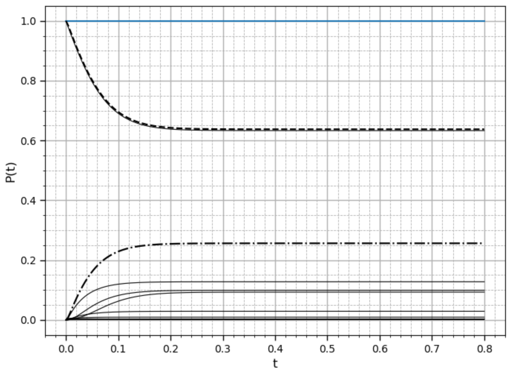
(2) The average service rate $\mu =11.3$ packets/s; the average packet arrival rate $\lambda =139.04$ packets/s. For this case, the modulus minimum characteristic exponent is ${\gamma }_{min}=-14.7$. The results of calculating the probabilities of states are presented in Figure 5. The probability of loss, varying from zero to $0.41$ during the transient, is equal to the probability that the buffer and the server are idle in the stationary mode. Solid lines indicate the probabilities of states. The time constant of the transient is ${\tau }_{max}=1⁄\left|{\gamma }_{min}\right|=1⁄14.7=0.068$ s, and the transient time is ${\tau }_{tr}=0.34$ s for $k=5$.

(3) The average service rate $\mu =33.33$ packets/s; the average packet arrival rate $\lambda =139.04$ packets/s. As a result of the calculation, it is found that ${\gamma }_{min}=-28.55$. The results of calculating the state probabilities are presented in Figure 6. Solid lines indicate the probabilities of system states. The probability of losses during the transient mode increases from zero at $t=0$ s to $0.26$ at $t>0.18$ s (see Figure 6). The probability that the system is free changes from unity at $t=0$ s to $0.64$ at $t>0.18$ s. The time constant for this case is ${\tau }_{max}=1⁄\left|{\gamma }_{min}\right|=1⁄28.55=0.035$ s, and the transient time is ${\tau }_{tr}=0.18$ s for $k=5$.

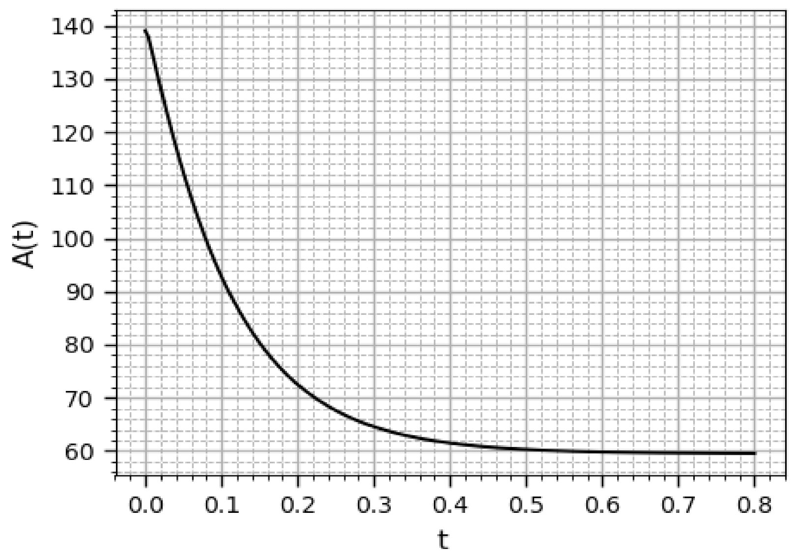
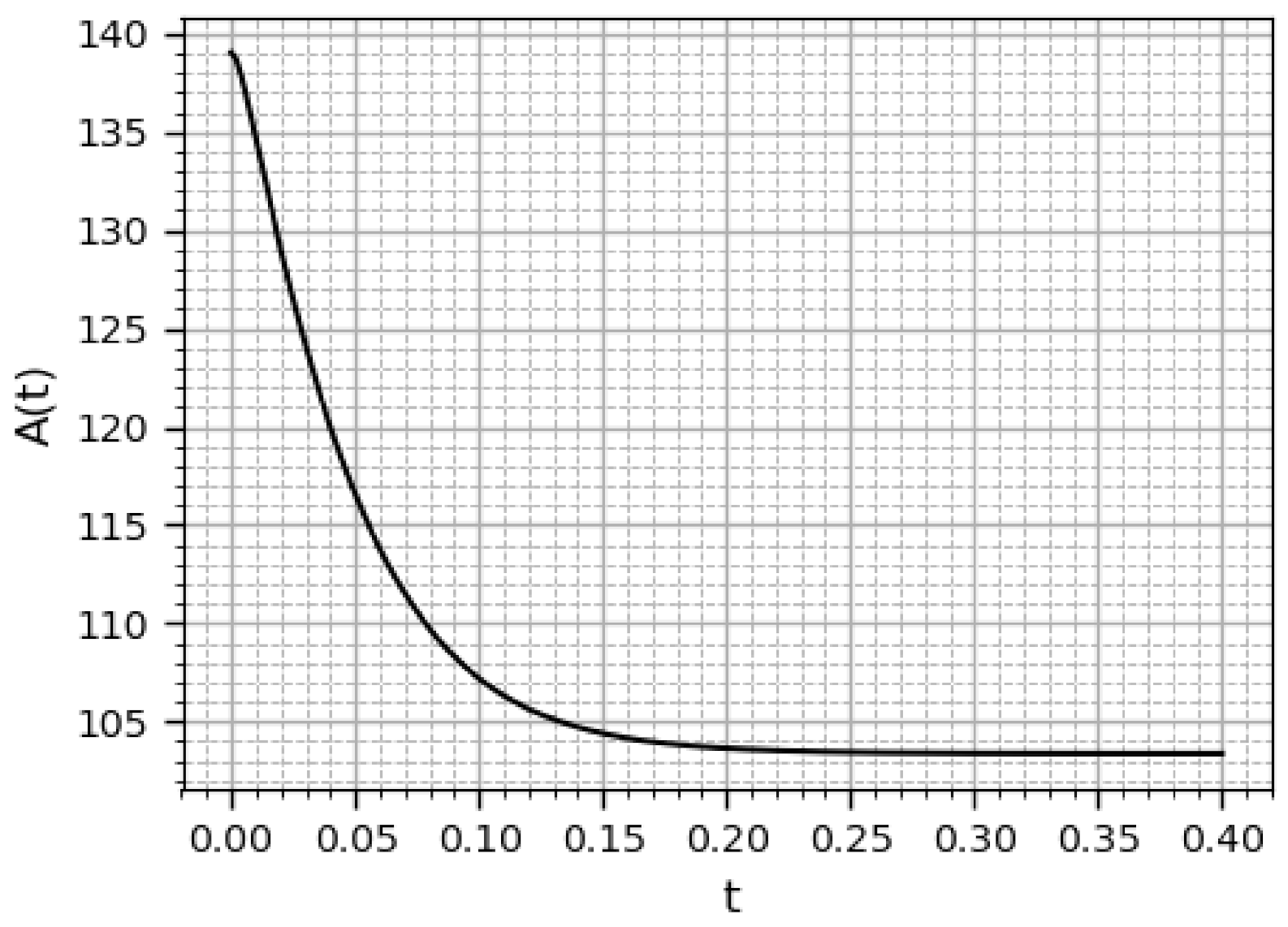
The results of studying the throughput of the system in the transient mode at $\mu =5$ packets/s and $\lambda =33.33$ packets/s are presented in Figure 7 and Figure 8, respectively. The throughput in the first case decreases from $A\left(0\right)=139.04$ packets/s to $A\left(t_{tr}\right)=59.9$ packets/s, and in the second case from $A\left(0\right)=139.04$ packets/s to $A\left(t_{tr}\right)=103.4$ packets/s.

Thus, with an increase in the service rate $\mu$, the transition time decreases. It should be noted that the transient time is long for high-speed data transmission systems, amounting to tenths of a second. In addition, the throughput of the system at the beginning of the system startup or reboot significantly exceeds the stationary value, which requires large resources for its processing. It follows from this that analysis of the characteristics of the system in the transient mode is necessary for the correct choice of the system configuration that provides the required quality of service indicators.

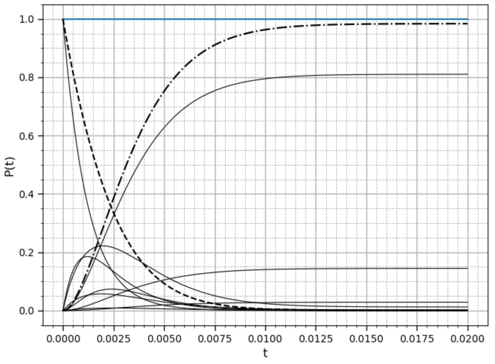
Consider the cases when any of ${\gamma }_k,k=\overline{0,K-1}$ is complex. This case corresponds, for example, to ${\lambda }_0={\lambda }_1={\lambda }_2=833$ packets/s, $\lambda =472.3$ packets/s, $\mu =11.3$ packets/s (Figure 9). In this case, there are four pairwise complex conjugate roots of the characteristic equation: ${\gamma }_{1,2}=-983.25\pm i81.86$, ${\gamma }_3,4=-894.92\pm i74.1$. The transient time is ${\tau }_{tr}=0.01$ s. Note that for these values of ${\tau }_k$ in the transient mode, there are bursts of probabilities that the server and the switch buffer are idle, along with the likelihood that the server is busy and the buffer is free for all types of traffic. At the same time, the values of some probabilities differ significantly from their values in the stationary mode. Thus, only the analysis of the behavior of the $MAP/M/1/N$ system in a stationary mode can lead to an incorrect assessment of the system state.

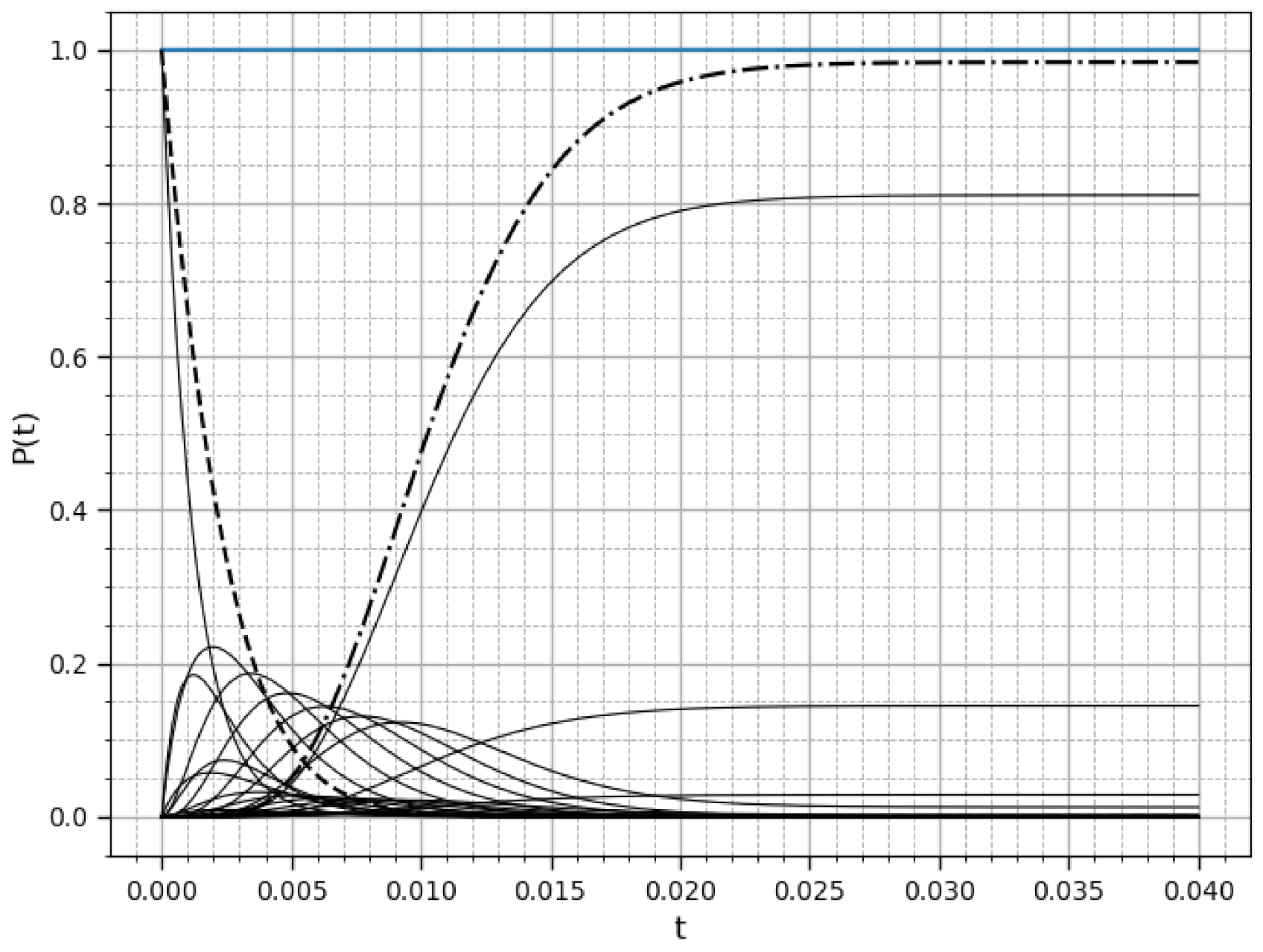
Increasing the size of the switch buffer obviously leads to a decrease in the probability of losses; however, it also causes a significant increase in the transient time. Thus, Figure 10 shows the results for the previous values of the intensities and transition probabilities, and $N=8$. The transient time is already ${\tau }_{tr}=0.025$ s with a slight decrease in the probability of losses.

6. Conclusions

This work was devoted to an analytical study of the transient mode of the $MAP/M/1$$/N$ system. First of all, based on the analysis of the Kolmogorov system of equations, it was shown that in such a system, there will always be a stationary mode. The paper presented for the first time an analytical method for studying the $MAP/M/1/N$ system in a transient mode, based on the concept of the so-called transformation matrix. Numerical methods were used only when calculating the eigenvalues of the coefficient matrix of the Kolmogorov system of equations for large-scale systems. Indeed, an algebraic equation higher than the fourth order has no analytical solution. The paper presents analytical expressions for calculating the time of the transient mode and the analysis of the possible behavior of the system in the transient mode, depending on the values of the roots of the characteristic equation of the system of Kolmogorov equations. Analytical expressions for calculating the probabilities of system states in a transient mode were presented. Analytical expressions were also presented for calculating the main indicators of the system operation, such as the probability of losses, throughput, the number of applications in the system at an arbitrary point in time, and the average values of throughput and the number of applications in the transient mode. Numerical modeling was carried out using the example of the $MAP/M/1/1$ system.

References

1. Dudin, A.N.; Klimenok, V.I.; Vishnevsky, V.M. Methods to Study Queuing Systems with Correlated Arrivals; Springer: Berlin/Heidelberg, Germany, 2020; 410p. [Google Scholar]
2. Lakatos, L.; Szeidl, L.; Telek, M. Introduction to Queueing Systems with Telecommunication Applications; Springer Science+Business Media, LCC: Berlin/Heidelberg, Germany, 2013; 385p. [Google Scholar]
3. Giambene, G. Queuing Theory and Telecommunications; Springer International Publishing: Berlin/Heidelberg, Germany, 2014; 516p. [Google Scholar]
4. Cohen, J.W. The Single Server Queue, 2nd ed.; Elsevier: Amsterdam, The Netherlands, 2012; 694p. [Google Scholar]
5. Prabhu, N.U. Queues and Inventories; John Wiley & Sons, Inc.: New York, NY, USA, 1965; 275p. [Google Scholar]
6. Harrison, P.G. Transient Behaviour of Queuing Networks. J. Appl. Probab. 1981, 18, 482–490. [Google Scholar] [CrossRef]
7. Abate, J.; Whitt, W. Transient behavior of the M/M/1 queue: Starting at the origin. Queuing Syst. 1987, 2, 41–65. [Google Scholar] [CrossRef]
8. Ammar, S.I.; Zeifman, A.; Satin, Y.; Kiseleva, K.; Korolev, V. On limiting characteristics for a non-stationary two-processor heterogeneous system with catastrophes, server failures and repairs. J. Ind. Manag. Optim. 2021, 17, 1057–1068. [Google Scholar]
9. Zeifman, A.; Satin, Y.; Kryukova, A.; Kiseleva, K.; Shilova, G. On Three Methods for Bounding the Rate of Convergence for Some Continuous-Time Markov Chains. Int. J. Appl. Math. Comput. Sci. 2020, 30, 251–266. [Google Scholar]
10. Zeifman, A. Stability for continuous-time nonhomogeneous Markov chains. In Stability Problems for Stochastic Models; Springer: Berlin/Heidelberg, Germany, 1985; pp. 401–414. [Google Scholar]
11. Kartashov, N.V. Strongly stable Markov chains. In Stability Problems for Stochastic Models; Institute for Systems Studies: Moscow, Russia, 1981; pp. 54–59. (In Russian) [Google Scholar]
12. Horváth, A.; Angius, A. Approximate transient analysis of queuing networks by decomposition based on time-inhomogeneous Markov arrival processes. EAI Endorsed Trans. Internet Things 2015, 1. [Google Scholar] [CrossRef] [Green Version]
13. Nilsen, F.B. Queuing Systems: Modeling, Analysis and Simulation; Springer: Berlin/Heidelberg, Germany, 1998; 43p. [Google Scholar]
14. Kumar, B.K.; Arivudainambi, D. Transient Solution of an M/M/1 Queue with Catastrophes. Comput. Math. Appl. 2000, 40, 1233–1240. [Google Scholar] [CrossRef] [Green Version]
15. Sophia, S. Transient analysis of a single server queue with chain sequence rates subject to catastrophes, failures and repairs. Int. J. Pure Appl. Math. 2018, 119, 1969–1988. [Google Scholar]
16. Kumar, B.K.; Krishnamoorthy, A.; Madheswari, S.P.; Basha, S.S. Transient Analysis of a Single Server Queue with Catastrophes, Failures and Repairs. Queueing Syst. Theory Appl. 2007, 56, 133–141. [Google Scholar] [CrossRef]
17. Kumar, R.; Sharma, S.; Rykov, V. Solution of a Heterogeneous Queuing System with Balking and Retention of Reneging Customers. Computer Networks. In Proceedings of the 26th International Conference, Sydney, NSW, Australia, 12–15 December 2019; pp. 330–346. [Google Scholar]
18. Rubino, G. Transient analysis of Markovian queueing systems: A survey with focus on closed forms and uniformization. In Queueing Theory 2: Advanced Trends; Wiley-ISTE: Hoboken, NJ, USA, 2021; pp. 269–307. [Google Scholar]
19. Kumar, R.; Soodan, B.S. Transient Analysis of a Single-Server Queuing System with Correlated Inputs and Reneging. Reliab. Theory Appl. 2019, 1, 102–106. [Google Scholar]
20. Nagy, G. Ordinary Differential Equations; Mathematics Department, Michigan State University: Michigan, MI, USA, 2021. [Google Scholar]
21. Ross, S.L. Differential Equations; John Waley & Sons Inc.: Hoboken, NJ, USA, 2004; 808p. [Google Scholar]
22. Ross, S.L. Introduction in to Ordinary Differential Equations; John Waley & Sons Inc.: Hoboken, NJ, USA, 1989; 620p. [Google Scholar]
23. Johnston, N. Advanced Linear and Matrix Algebra; Springer Nature: Cham, Switzerland, 2021; 494p. [Google Scholar]
24. Gantmacher, F.R. The Theory of Matrices. Vol.1, Vol.2.; Chelsea Publishing Company: New York, NY, USA, 1959; Volume 1, 374p, Volume 2, 277p. [Google Scholar]
25. Kwong, M.K.; Zettl, A. New proofs and extensions of sylvester’s and johnson’s inertia theorems to non-hermitian matrices. Proc. Am. Math. Soc. 2011, 139, 3795–3806. [Google Scholar] [CrossRef] [Green Version]
26. Nieuwenhuis, H.J.; Schoonbeek, L. Stability of matrices with negative diagonal submatrices. Linear Algebra Appl. 2002, 353, 183–196. [Google Scholar] [CrossRef] [Green Version]
27. Nieuwenhuis, H.J.; Schoonbeek, L. Stability of matrices with sufficiently strong negative-dominantdiagonal submatrices. Linear Algebra Appl. 1997, 258, 195–217. [Google Scholar] [CrossRef] [Green Version]
Figure 1. Generalized graph of the M A P / M / 1 / N queuing system.
Mathematics 09 02559 g001
Figure 2. Types of transient modes.
Mathematics 09 02559 g002
Figure 3. Transition graph of the M A P / M / 1 / N system.
Mathematics 09 02559 g003
Figure 4. Dependencies of the probabilities on the time. Dashed and dotted line—the probability of losses; dashed line—the servicing device is idle, the buffer is empty.
Mathematics 09 02559 g004
Figure 5. Dependencies of the probabilities on the time. Dashed and dotted line—the probability of losses; dashed line—the servicing device is idle, the buffer is empty.
Mathematics 09 02559 g005
Figure 6. Dependencies of the probabilities on the time. Dashed and dotted line—the probability of losses; dashed line—the servicing device is idle, the buffer is empty.
Mathematics 09 02559 g006
Figure 7. Dependence of the system throughput on time.
Mathematics 09 02559 g007
Figure 8. Dependence of the system throughput on time.
Mathematics 09 02559 g008
Figure 9. Dependencies of the probabilities on the time. Dashed and dotted line—the probability of losses; dashed line—the servicing device is idle, the buffer is empty.
Mathematics 09 02559 g009
Figure 10. Dependencies of the probabilities on the time. Dashed and dotted line—the probability of losses; dashed line—the servicing device is idle, the buffer is empty.
Mathematics 09 02559 g010
Publisher’s Note: MDPI stays neutral with regard to jurisdictional claims in published maps and institutional affiliations.