1. Introduction
Turbulence is most likely the open subject in physics with the greatest number of applications in everyday life. Turbulent flows are inherent in practically any flow in engineering, but they are also critical in meteorology and pollutant dispersion [
1]. It is known that we still lack an existence and uniqueness theorem for the solution of the Navier–Stokes equations, which govern the behaviour of turbulent flows [
2]. Furthermore, apart from a few trivial examples, these equations cannot be solved analytically [
1].
It is also well known that turbulent-flow simulations can be considered in terms of three levels of detail: RANS (Reynolds-averaged Navier–Stokes) [
3], LES (large-eddy simulation) [
4], and DNS (direct numerical simulation) [
5,
6], each of which corresponds to a different level of accuracy. Nevertheless, until now, DNS has been the only method that has been proven to be reliable for investigating the physical properties of flows that are still poorly understood. On the other hand, DNSs are extremely expensive because every turbulent scale in the flow, both temporal and spatial, must be properly resolved. This requires very fine grids and very small temporal steps. Furthermore, as a result of the evolution of the Kolmogorov scales (the smallest turbulent scale) [
7,
8], the number of points required to perform the simulation grows extremely quickly, as
, where
is the Reynolds number. As a result, using DNS to understand turbulent flows requires considering simple geometries, allowing for very precise and fast numerical tools, such as the ones described in this paper. Pipe, channel, and flat-plate boundary layers are examples of canonical wall-bounded flows. A slightly more complex flow case is the square duct [
9,
10,
11], which is very relevant due to the presence of Prandtl’s secondary flow of second kind [
12]. The secondary flow in ducts consists of non-vanishing values of the mean cross-stream velocity components, sharing some similarities with the ones present in Couette flows [
13,
14,
15,
16]. Due to the presence of the side walls, turbulent ducts are more challenging to simulate [
17,
18,
19] than channels, pipes, or boundary layers. This method, like many other high-resolution ones, cannot be used in complex geometries. A hole in the domain, for example, would render this method inapplicable. See [
20] for details.
The behaviour of turbulent flows is described by the Navier–Stokes equations, which are composed by the continuity and momentum equations:
where
are the velocity components (
U,
V and
W in the streamwise, spanwise and wall-normal directions, respectively),
P is the pressure, and
is the Reynolds number of the problem. Note that in the following
x,
y, and
z are the streamwise, wall-normal and spanwise components, respectively. These equations can be transformed for simple domains [
21,
22] into the vorticity-Laplacian form, see also [
23]. In such geometries, one can take advantage of the derived formulation in the
y component of the vorticity
, and the bi-Laplacian of the wall-normal velocity
, as explained in Ref. [
21]. The main advantages of this method are that the pressure does not need to be explicitly computed, removing staggered grids, and that only these two fields are needed to follow the evolution of the turbulent flow. The equations become:
where
and
collect the nonlinear part of the Equations (
1) and (
2) [
22]. For instance, in turbulent channel flow, there are two periodic directions that allow the use of fast-Fourier methods in these directions. This method was used in the first large DNS of wall turbulence [
21], and in many more after that [
5,
22,
24]. Using Fourier methods, instead of solving one large equation one has to solve millions of one-dimensional (1D) equations.
In order to solve these many elliptical problems, compact finite difference (CFD) schemes [
25] have been one of the most important tools. Briefly, the main difference between compact and normal finite differences is that the former also considers a stencil in the derivative. Due to their flexibility and high accuracy, CFD schemes have become a very important tool for solving partial-differential-equation problems [
26,
27,
28].
However, in the case of square (or rectangular) ducts, only the streamwise direction is periodic. Thus, fast-Fourier-transform (FFT) techniques can only be used in this direction, obtaining thousands, instead of millions, of two-dimensional (2D), fourth-order, elliptical problems. Our objective is thus to obtain a method that uses the power and memory of new computers for efficiently solving this problem. Moreover, as it is shown below the boundary conditions (BC) of the problem are both Dirchlet and Neumann homogeneous. We propose an efficient algorithm to impose Neumann BC, taking advantage of the capabilities of CFD to compute any kind of derivatives. Note that our methods are general and can be applied to any other fourth-order elliptic problem, like the bending of beams [
29,
30,
31].
In the second section, the method is explained in detail: First, we will briefly explain the one-dimensional CFD methods. Then, we explain the discretization of the problem, and the boundary value problem. The validation is detailed in the third section. Finally, conclusions and future work are given in section four.
2. Methods
The geometry of a rectangular duct is shown in
Figure 1 (left) together with a sketch of the two-dimensional plane where we solve the bi-Laplacian problem (right panel). The flow is periodic in the streamwise direction and at rest at the walls. The dimensions of the box are
,
and
in the streamwise, wall-normal, and spanwise directions, respectively.
D is usually taken large enough to avoid spurious effects due to the periodicity of the box. Equations (
3) and (
4) are solved together, but in this case, we will focus on Equation (
3). Using the auxiliary function
, the problem becomes:
In Fourier space, these equations transform into
problems, where
is the size of the transform, which takes the form:
In these equations,
is the
k-th mode of the Fourier transform of the nonlinear term, which is not usually easy to compute [
22]. Note that this allows us to very efficiently distribute these problems in a large supercomputer, as every node has just a few problems to solve, generally one. Applying any time-stepper, with explicit linear solver and implicit non-linear one (see for example Ref. [
32]), and removing the hats for simplicity, (
7) and (
8) transform into:
In this equation,
stands for the RHS of the time stepper [
32]. Note that
is a constant, subsuming the Reynolds number, wavenumber
k, temporal step
, and any constant coming from the temporal-discretization method. For the case of the duct, the boundary conditions for
V are Dirichlet and Neumann homogeneous. These boundary conditions come directly from the continuity Equation (
1) and the non-slip condition. While the imposition of the former is relatively easy, the latter cannot be imposed directly in the resolution of the problem. Furthermore, note that there are no boundary conditions for
. The final problem, removing the
n for simplicity, is then:
2.1. Compact-Finite-Difference Methods
The CFD method was introduced in a groundbreaking article by S.K. Lele in 1992 [
25]. Lele’s idea was to use finite-difference methods to solve problems exhibiting a wide range of spatial scales, generalizing some Padé schemes that had been used earlier [
33,
34]. Lele’s CFD main advantage is that, as opposed to to spectral methods, the location of the points is free, exhibiting similar accuracy. The most important fact about CFD methods is that they impose a linear relationship between the values of the derivatives at any order of the function and the value of the function in the vicinity of all points, i.e., for point
we have:
In this equation,
d and
f are the semi-size of the stencil, and
is the derivative of order
l evaluated at
. Using Taylor’s theorem as in Ref. [
22], it is possible to obtain two sparse matrices such that:
However, it is impossible to repeat this procedure for 2D stencils due to a lack of resolution near the corners of the domain. Thus, the option is to employ 1D discretization in the two directions. Assuming that
for
the nodes are distributed in the following way:
In this equation, the bold face is used to indicate that the data is distributed as a two-dimensional array. Using Equation (
16), it is possible to define eight matrices such that:
where the superscript indicates a partial derivative in that particular direction.
2.2. Discretization
The discretization of Equations (
11) and (
12) is similar but, as the former is more general, we will explain only this one. Expanding Equation (
11) yields:
Left-multiplying this equation by
and right-multiplying it by
, one gets:
Using now the properties of these CFD matrices, shown in (
17), we get
Using these two equations in (
19), the derivatives can be removed from the equation:
The next step is to transform this problem into a linear equation of the form
. The first step is to define an operator, ⊗, as
Using coordinates we have,
Defining now
as
we obtain:
Note that this algorithm can (and must) be simplified, as all the involved matrices are sparse. The problem now becomes
To simplify this equation, we can define an array
and a last operator,
G, for the RHS.
G is defined as
so the problem (
21) becomes
Equation (
26) still includes the points on the boundary. Given a function
that summarises the Dirichlet boundary conditions, the value of
at the boundary is defined as:
thus, it is possible to decompose
as follows:
Returning to Equation (
26), we have:
where only the equations at the inner points make sense. This system can easily be transformed into a sparse algebraic problem of dimension
.
2.3. The Boundary Problem
The resolution of the problem (
11)–(
14) is straightforward in the case of Dirichlet boundary conditions. Moreover, the matrix
G does not depend on the boundary conditions. The method proposed here generalizes the method proposed in Ref. [
21]. The value of the normal derivative is built up using several auxiliary functions. In 1D problems, two auxiliary functions are enough. However, in 2D, many more are needed. Due to this, problems like the square duct have never been addressed using this technique. In this case, the solution is constructed as a linear combination of
fields:
The first field in the RHS is the particular solution of the system (
11)–(
14), with equations:
Here,
is Dirichlet homogeneous, but does not satisfy the Neumann condition. For any point
on the boundary, the homogeneous solution
is defined as:
As V is identically 0 on the boundary, eight of these functions, four corners and two directions, are identically zero, thus only fields need to be solved. Note that as these fields are solution of a homogeneus equation, we only need to compute them once at the beginning of the program and use them for every time step. This needs a constant time step , as the parameter usually depends on .
One of the main advantages of the CFD methods is that any derivative can be computed with very high accuracy. This allows us to compute the normal derivatives of the
functions:
Therefore, we obtain
equations, once for each point:
Applying now the boundary condition and solving for
, we obtain:
The matrix of this system is not sparse anymore, but has a relatively small size. The largest simulations of wall turbulence have around 2000 points in the wall-normal direction [
35], so this matrix has a maximum estimated dimension of
. This can be solved in seconds in a state-of-the-art computer. Notice also that due to the symmetries of the domain, many of the
fields can be computed using these symmetries instead of solving the system (
32). In the case of a square domain, only
of the fields are needed, as every other can be computed from these ones.
3. Results
The use of high-order numerical schemes such as CFD in fluid dynamics is essential when complex flow structures characterised by high gradients in the magnitudes being calculated appears. Accuracy is then, together with efficiency, the main objective pursued with the numerical method described in this work.
As noted in
Section 2.3, the methodology applied to impose the Neumann boundary conditions to a 2D domain and solve the bi-Laplacian operator requires the solution of many linear systems of equations. The only variation among them is the boundary conditions, which end up being part of the right-hand side of the system, remaining the matrix of the system unvaried. The extent to which one can take advantage of this characteristic will significantly determine the computational cost necessary to solve the bi-Laplacian operator. Moreover, the accuracy of the CFD method is defined by the employed stencil, which results in a specific truncation order of the Taylor expansion. The number of non-zero elements of the system matrices changes with the stencil dimension: for a stencil dimension
J the number of non-zero elements increases as
. As the computational cost increases with the non-zero elements existing in a sparse matrix, a balance between truncation order and computational cost must be found.
Among the different methodologies available to solve the non-symmetric linear systems of equations resulting from the spatial discretization and the implementation of the CFD schemes, the preconditioned generalized minimal residual (GMRES) method has been found to be the most suitable for the study case. This method is included in the SPARSEKIT2 package [
36], which contains many preconditioners that vary in computational cost and that fit different matrices according to their conditioning. In this study, the preconditioners that best fit the generated matrices are, on the one hand, the incomplete factorization ILU(0) for preconditioning matrices
and
. On the other hand, the incomplete LU factorization with standard dropping strategy (ILUD) for the
matrices when solving the Laplacian operators. The main advantage of the ILU(0) preconditioner is its simplicity and low computational cost, suitable for matrices with good conditioning. For matrices with worse conditioning, the ILUD preconditioner offers a good ratio convergence/cost. An important advantage is that it provides the possibility to adjust the element-dropping tolerance for prioritizing the preconditioning cost or the convergence speed.
To test the precision with which the system (
11)–(
14) is being solved, a group of 2D solutions satisfying the Neumann and Dirichlet boundary conditions are set out:
where
are the function wave numbers.
This product of cosines guarantees that for any
, the value of
and its first wall-normal derivatives are null. This group of solutions is used to compose a suitable field
:
in such a way that when increasing the wave numbers, the gradients in the solution
and in the field
increase as well, see
Figure 2.
For sufficiently high wave numbers,
and
adopt a chaotic-like distribution similar to that of Gaussian white noise, thus emulating the gradients that could be found in a ducted flow at relatively high Reynolds numbers. System (
31) is solved for
and the numerical solution,
V is compared to
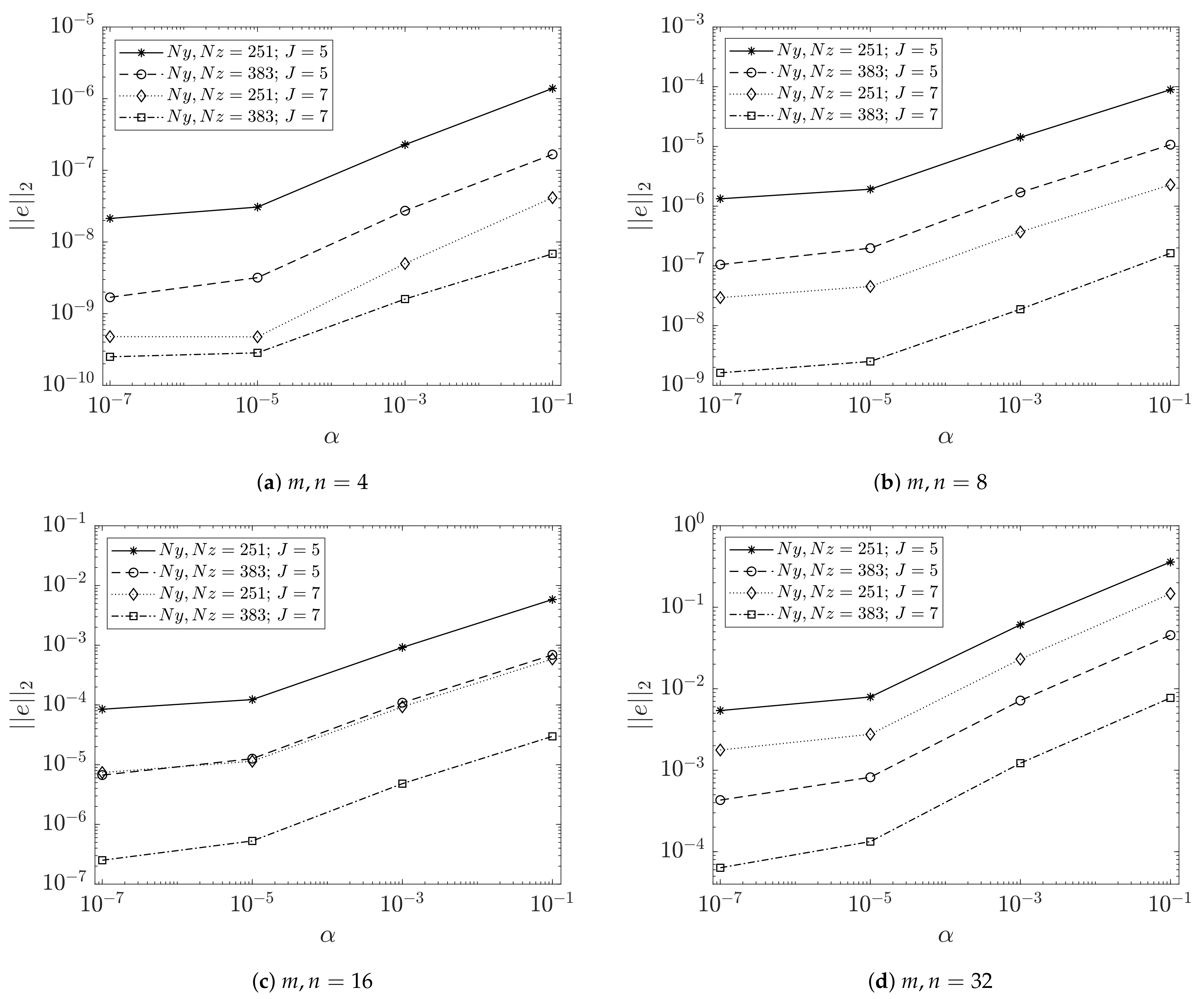
. To analyse this error, two different norms have been used: L2-norm relative error:
The relative error evolution with respect to
, as shown in
Figure 3, follows very similar trends among the different wave number, mesh resolution and stencil configurations. In all the configurations proposed, the increment of the relative error with
is significant in the range analysed, with about two orders of magnitude difference between the minimum value of
and the maximum one of
. In this range, there is a perceptible change of tendency; for
, the trends seem to be linear in a log-log representation, which is indicative of fitting a power function trend, while for
, the error reduction is less significant. These variations in the errors with
are directly related to the gradients that appear in
when applying the two Laplacian operators to the imposed solution
. When reducing the coefficient multiplying the second Laplacian, the effect of this is damped smoothing the gradients in
.
When comparing grid sizes and truncation orders through the stencil size J, in the range studied, increasing the grid size produces a decrease in the relative error of a similar order of magnitude to that of the increase in the truncation order. However, when comparing the error distributions for and , as the field gradients steepen, the lack of mesh resolution cannot be overcome by the truncation order. However, when the grid resolution is not excessively low with respect to the field gradients, the use of higher-order stencils leads to an important increase in accuracy.
The spatial distribution of the error is shown in
Figure 4. Here, we can see that the error is a heterogeneous field where the higher errors are found mainly in the interior part of the field, decreasing as getting closer to the boundaries. This heterogeneous and non-symmetric error field obtained when solving the bi-Laplacian operator for a symmetric field
is presumably related to the accuracy with which the system in (
35) is solved when obtaining the constants that will weigh each one of the homogeneous solutions. In this regard, a comparison between homogeneous solutions of
and
V is provided in
Figure 5. The damping of the homogeneous solution is much higher for
, making imperceptible the transition from the imposed boundary condition to the unaffected near field. In the case of
V, the gradients are smaller, extending the contribution of the homogeneous solution all over the field.
The high number of homogeneous solutions needed to guarantee that Neumann-homogeneous boundary conditions are satisfied implies saving fields in which a high percentage of elements are close to zero. In order to reduce these memory requirements, that increase with the number of boundary nodes, a filtering of the values that fall below a determined threshold, followed by a sparse storage of the surviving elements of the field could reduce these requirements. However, as shown in field V, the effect of homogeneous solutions spreads all over the field. Therefore a reduction in the accuracy of the method can be expected. In case memory resources constitute an impediment to complete a simulation, deeper studies must be performed to evaluate the accuracy reduction associated to this procedure applied to the specific problem.


