
Model-Assisted Labeling and Self-Training for Label Noise Reduction in the Detection of Stains on Images of Laundry


Abstract
:1. Introduction
1.1. Weakly Supervised Learning
1.2. Considering Label Noise
1.3. Self-Training
1.4. Hybrid Approaches
1.5. Our Approach
- Unique properties of the domain of stain detection on flat and patterned laundry are pointed out.
- The reduction in label noise with the help of predictions by a model is evaluated in two experiments:
- Model-assisted labeling (MAL) [33]: A human is simulated as selecting overlooked stains from the predictions of the model. This approach provides a baseline for autonomous approaches and shows that predictions can be used for semi-automated labeling.
- High Certainty: Regions predicted with high certainty are automatically incorporated into the labels. This approach conforms to dealing with noisy labels via self-training.
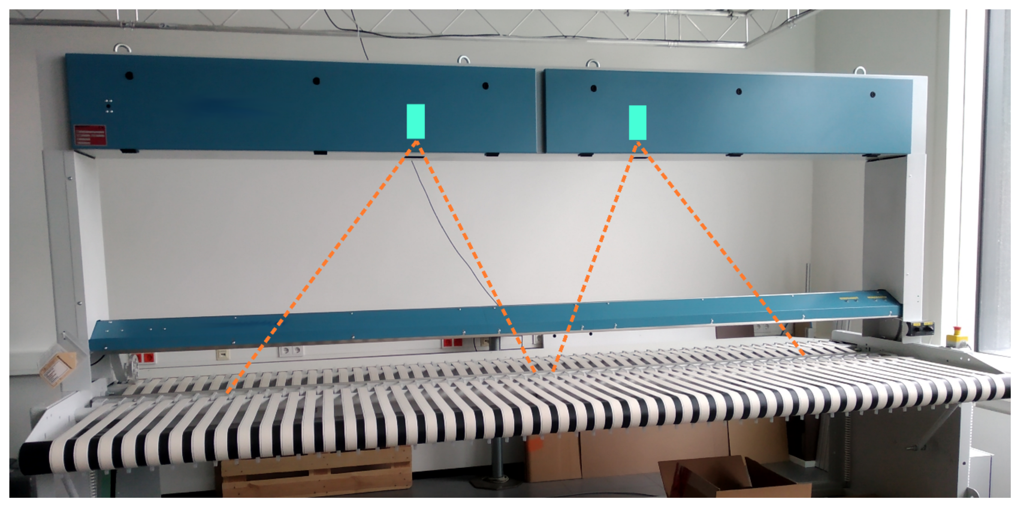
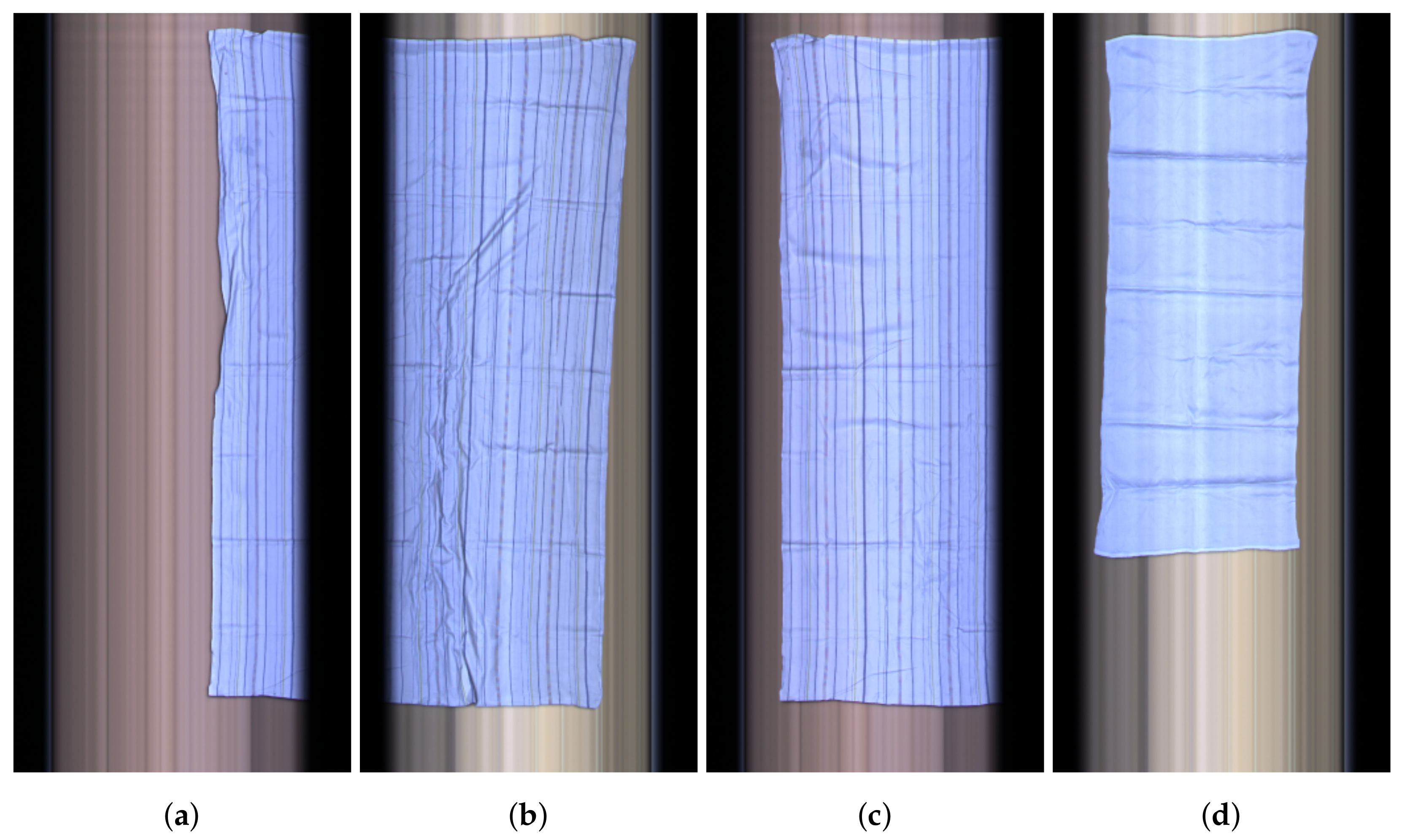
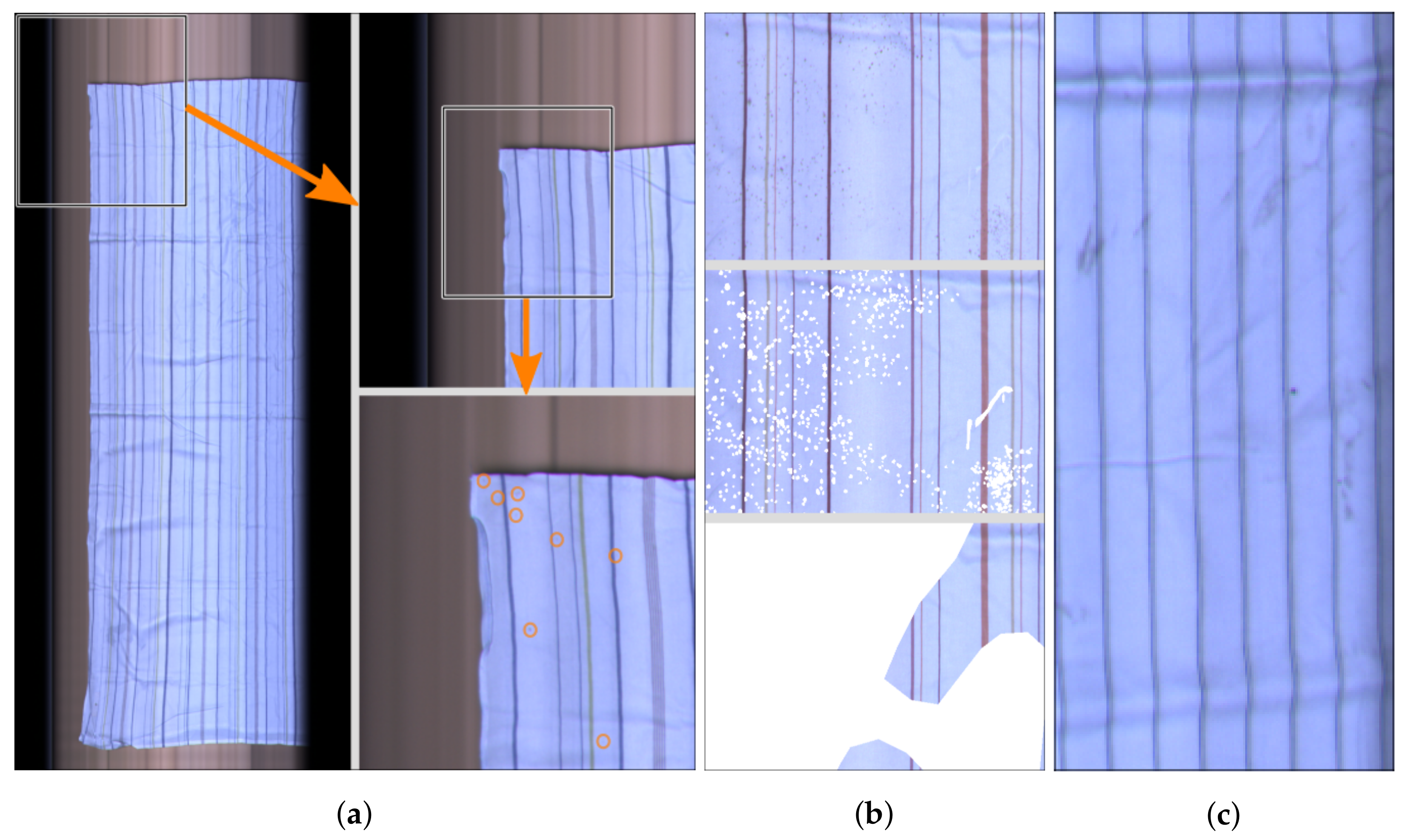
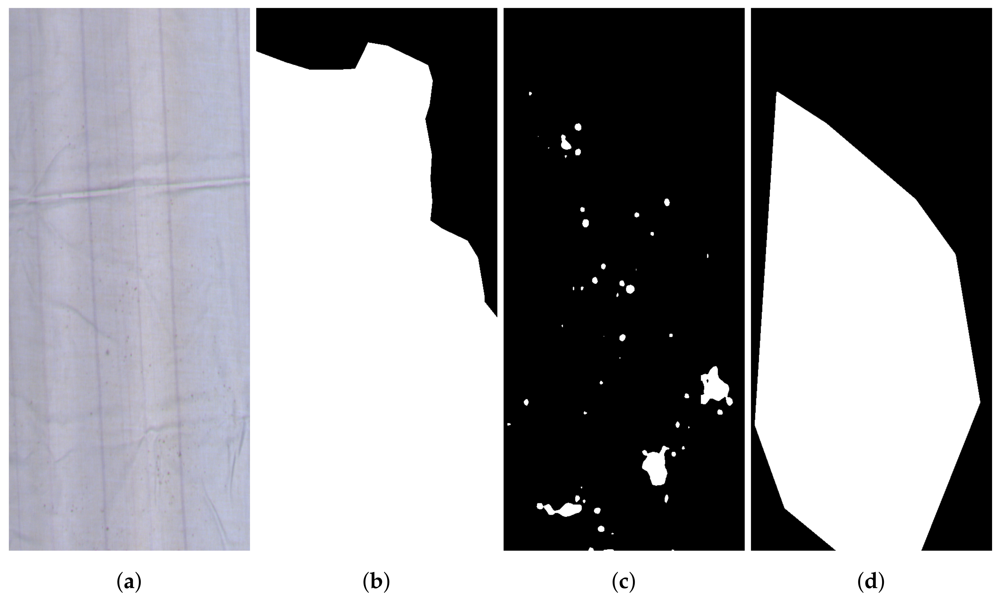
2. A Dataset for Stain Detection
3. Model Training
4. Experiments
- A model is trained on the training split of the dataset with the initial labels and the weights from the epoch yielding the best results on the validation split with the revised labels are selected.
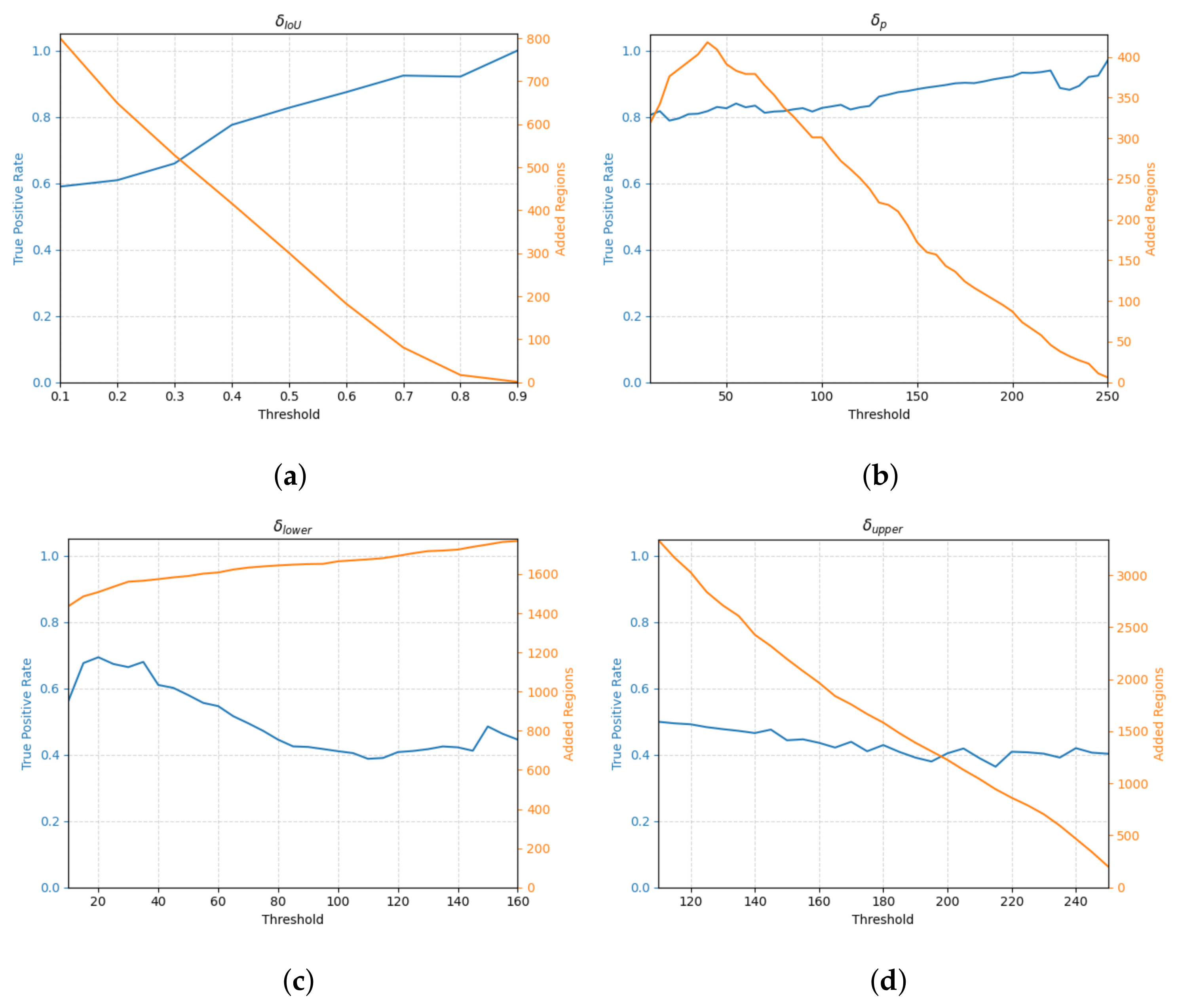
- The predictions P of the model on the training images are combined with the initial Labels to create a model-revised labeling . Different label revision functions are used for the MAL and the self-training experiment.
- A new model is trained on the training split of the dataset with the model-revised labels and the weights from the epoch yielding the best results on the validation split with the revised labels are selected.
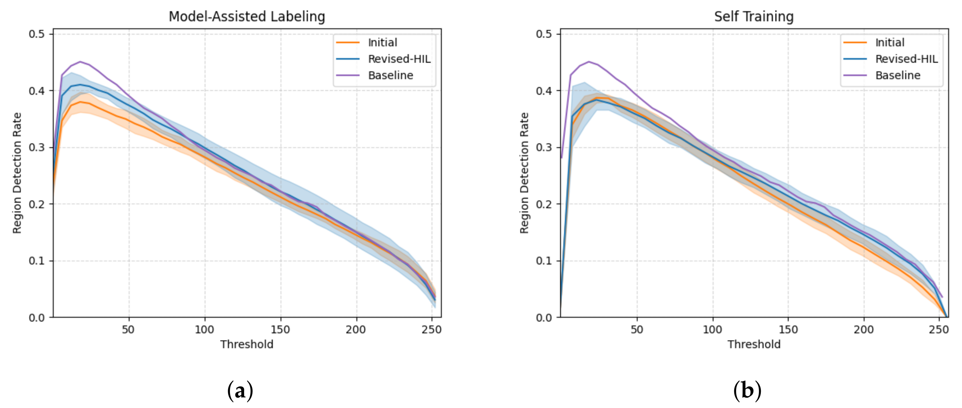
- The results of and on the validation split with the revised labels are compared to see if training with the model-revised labels increased the overall performance.
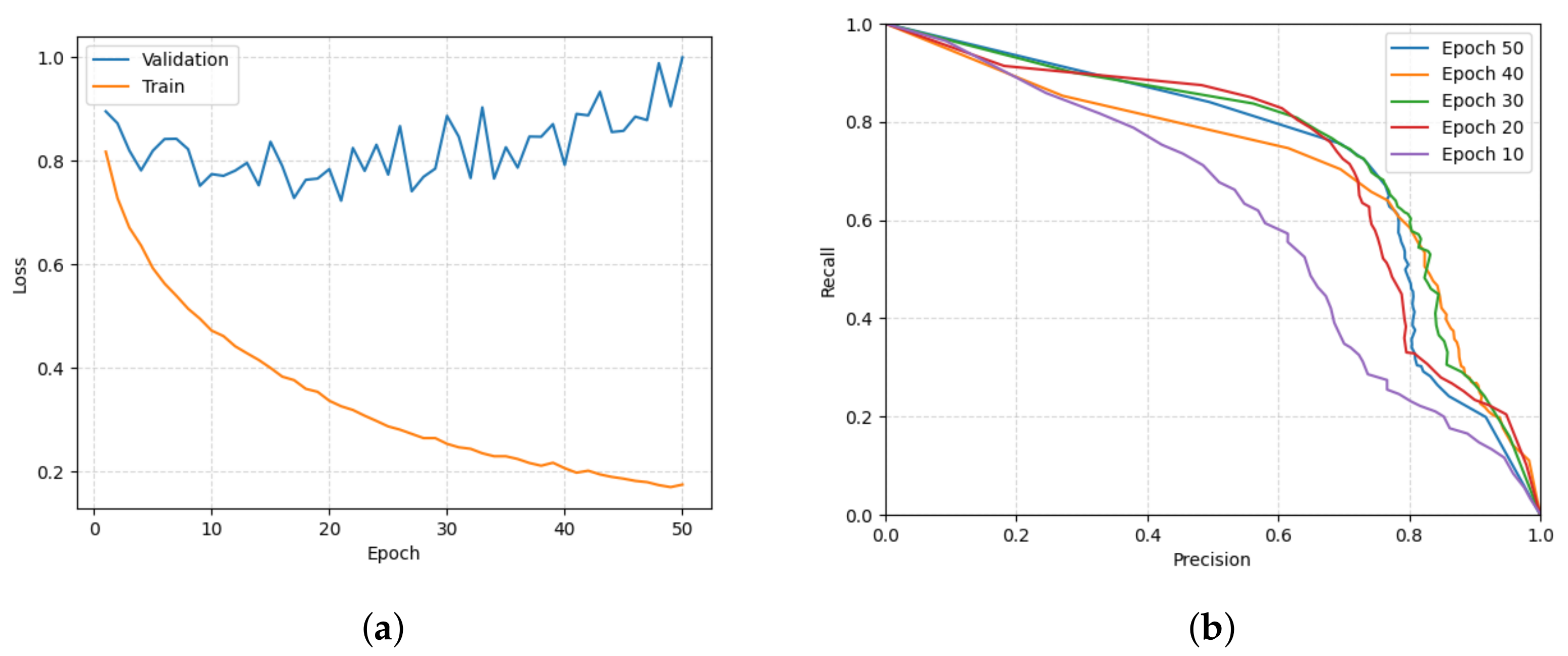
5. Results and Discussion
6. Conclusions
- Is it possible to refine rough regions and to remove erroneous regions in addition to adding overlooked regions?
- Is it possible to apply MAL during the initial labeling by training a model with limited data and then using it to make suggestions, as was carried out by Hasty [42]?
- Can self-training be successfully applied by either using a different approach to selecting predicted regions or by filtering false positives from highly certain predictions?
Author Contributions
Funding
Institutional Review Board Statement
Informed Consent Statement
Data Availability Statement
Acknowledgments

Conflicts of Interest
Abbreviations
| AUC | area under curve |
| CPD | Cascaded Partial Decoder |
| IoU | intersection over union |
| MAE | mean absolute error |
| MAL | model-assisted labeling |
| PR | precision-recall |
| RDR | region detection rate |
| SOD | salient object detection |
| TPR | true positive rate |
| CNN | Convolutional Neural Network |
References
- Wu, Z.; Su, L.; Huang, Q. Cascaded Partial Decoder for Fast and Accurate Salient Object Detection. In Proceedings of the IEEE Conference on Computer Vision and Pattern Recognition, Long Beach, CA, USA, 15–20 June 2019; pp. 3907–3916. [Google Scholar]
- Qin, X.; Zhang, Z.; Huang, C.; Gao, C.; Dehghan, M.; Jagersand, M. BASNet: Boundary-Aware Salient Object Detection. In Proceedings of the IEEE/CVF Conference on Computer Vision and Pattern Recognition, Long Beach, CA, USA, 15–20 June 2019; pp. 7479–7489. [Google Scholar]
- Qin, X.; Zhang, Z.; Huang, C.; Dehghan, M.; Zaiane, O.R.; Jagersand, M. U2-Net: Going deeper with nested U-structure for salient object detection. Pattern Recog. 2020, 106, 107404. [Google Scholar] [CrossRef]
- Zoph, B.; Ghiasi, G.; Lin, T.Y.; Cui, Y.; Liu, H.; Cubuk, E.D.; Le, Q. Rethinking Pre-training and Self-training. arXiv 2020, arXiv:2006.06882. [Google Scholar]
- Tao, A.; Sapra, K.; Catanzaro, B. Hierarchical Multi-Scale Attention for Semantic Segmentation. arXiv 2020, arXiv:2005.10821. [Google Scholar]
- Huang, Y.; Jia, W.; He, X.; Liu, L.; Li, Y.; Tao, D. Channelized Axial Attention for Semantic Segmentation. arXiv 2021, arXiv:2101.07434. [Google Scholar]
- Bagherinezhad, H.; Horton, M.; Rastegari, M.; Farhadi, A. Label Refinery: Improving ImageNet Classification through Label Progression. arXiv 2018, arXiv:1805.02641. [Google Scholar]
- Khoreva, A.; Benenson, R.; Hosang, J.; Hein, M.; Schiele, B. Simple Does It: Weakly Supervised Instance and Semantic Segmentation. In Proceedings of the IEEE Conference on Computer Vision and Pattern Recognition, Honolulu, HI, USA, 21–26 July 2017; pp. 876–885. [Google Scholar]
- Pont-Tuset, J.; Arbeláez, P.; Barron, J.T.; Marques, F.; Malik, J. Multiscale Combinatorial Grouping for Image Segmentation and Object Proposal Generation. IEEE Trans. Pattern Anal. Mach. Intell. 2017, 39, 128–140. [Google Scholar] [CrossRef] [PubMed] [Green Version]
- Rother, C.; Kolmogorov, V.; Blake, A. “GrabCut”: Interactive Foreground Extraction Using Iterated Graph Cuts; ACM SIGGRAPH 2004 Papers; ACM: New York, NY, USA, 2004; pp. 309–314. [Google Scholar] [CrossRef]
- Chen, L.C.; Papandreou, G.; Kokkinos, I.; Murphy, K.; Yuille, A.L. DeepLab: Semantic Image Segmentation with Deep Convolutional Nets, Atrous Convolution, and Fully Connected CRFs. IEEE Trans. Pattern Anal. Mach. Intell. 2018, 40, 834–848. [Google Scholar] [CrossRef] [PubMed]
- Hsu, C.C.; Hsu, K.J.; Tsai, C.C.; Lin, Y.Y.; Chuang, Y.Y. Weakly Supervised Instance Segmentation using the Bounding Box Tightness Prior. In Advances in Neural Information Processing Systems 32; Wallach, H., Larochelle, H., Beygelzimer, A., Alché-Buc, F.d., Fox, E., Garnett, R., Eds.; Curran Associates, Inc.: Red Hook, NY, USA, 2019; pp. 6586–6597. [Google Scholar]
- He, K.; Gkioxari, G.; Dollar, P.; Girshick, R. Mask R-CNN. In Proceedings of the IEEE International Conference on Computer Vision, Venice, Italy, 22–27 October 2017; pp. 2961–2969. [Google Scholar]
- Lu, Z.; Fu, Z.; Xiang, T.; Han, P.; Wang, L.; Gao, X. Learning from Weak and Noisy Labels for Semantic Segmentation. IEEE Trans. Pattern Anal. Mac. Intell. 2017, 39, 486–500. [Google Scholar] [CrossRef] [PubMed] [Green Version]
- Wang, L.; Lu, H.; Wang, Y.; Feng, M.; Wang, D.; Yin, B.; Ruan, X. Learning to Detect Salient Objects With Image-Level Supervision. In Proceedings of the IEEE Conference on Computer Vision and Pattern Recognition, Honolulu, HI, USA, 21–26 July 2017; pp. 136–145. [Google Scholar]
- Bekker, A.J.; Goldberger, J. Training deep neural-networks based on unreliable labels. In Proceedings of the 2016 IEEE International Conference on Acoustics, Speech and Signal Processing (ICASSP), Shanghai, China, 20–25 March 2016; pp. 2682–2686. [Google Scholar] [CrossRef]
- Zhang, J.; Zhang, T.; Daf, Y.; Harandi, M.; Hartley, R. Deep Unsupervised Saliency Detection: A Multiple Noisy Labeling Perspective. In Proceedings of the 2018 IEEE/CVF Conference on Computer Vision and Pattern Recognition, Salt Lake City, UT, USA, 18–22 June 2018; pp. 9029–9038. [Google Scholar] [CrossRef] [Green Version]
- Han, J.; Luo, P.; Wang, X. Deep Self-Learning From Noisy Labels. In Proceedings of the IEEE/CVF International Conference on Computer Vision, Seoul, Korea, 27–28 October 2019; pp. 5138–5147. [Google Scholar]
- Luo, A.; Li, X.; Yang, F.; Jiao, Z.; Cheng, H. Webly-supervised learning for salient object detection. Pattern Recog. 2020, 103, 107308. [Google Scholar] [CrossRef]
- Barnes, C.; Shechtman, E.; Finkelstein, A.; Goldman, D.B. PatchMatch: A Randomized Correspondence Algorithm for Structural Image Editing; ACM SIGGRAPH 2009 Papers; Association for Computing Machinery: New York, NY, USA, 2009; pp. 1–11. [Google Scholar] [CrossRef]
- Yi, R.; Huang, Y.; Guan, Q.; Pu, M.; Zhang, R. Learning from Pixel-Level Label Noise: A New Perspective for Semi-Supervised Semantic Segmentation. arXiv 2021, arXiv:2103.14242. [Google Scholar]
- Zhou, B.; Khosla, A.; Lapedriza, A.; Oliva, A.; Torralba, A. Learning Deep Features for Discriminative Localization. In Proceedings of the IEEE Conference on Computer Vision and Pattern Recognition, Las Vegas, NV, USA, 27–30 June 2016; pp. 2921–2929. [Google Scholar]
- Rosenberg, C.; Hebert, M.; Schneiderman, H. Semi-Supervised Self-Training of Object Detection Models. In Proceedings of the 2005 Seventh IEEE Workshops on Applications of Computer Vision (WACV/MOTION’05), Washington, DC, USA, 5–7 January 2005; Volume 1, pp. 29–36. [Google Scholar] [CrossRef]
- Bengio, Y.; Louradour, J.; Collobert, R.; Weston, J. Curriculum learning. In Proceedings of the 26th Annual International Conference on Machine Learning, Association for Computing Machinery, Montreal, QC, Canada, 14–18 June 2009; pp. 41–48. [Google Scholar] [CrossRef]
- Zou, Y.; Yu, Z.; Kumar, B.V.K.V.; Wang, J. Unsupervised Domain Adaptation for Semantic Segmentation via Class-Balanced Self-Training. In Proceedings of the European Conference on Computer Vision (ECCV), Munich, Germany, 8–14 September 2018; pp. 289–305. [Google Scholar]
- Zou, Y.; Yu, Z.; Liu, X.; Kumar, B.V.K.V.; Wang, J. Confidence Regularized Self-Training. In Proceedings of the IEEE/CVF International Conference on Computer Vision (ICCV), Seoul, Korea, 27–28 October 2019; pp. 5982–5991. [Google Scholar]
- Huang, Y.; Qiu, C.; Guo, Y.; Wang, X.; Yuan, K. Surface Defect Saliency of Magnetic Tile. In Proceedings of the 2018 IEEE 14th International Conference on Automation Science and Engineering (CASE), Munich, Germany, 20–24 August 2018; pp. 612–617. [Google Scholar] [CrossRef]
- Bai, X.; Fang, Y.; Lin, W.; Wang, L.; Ju, B.F. Saliency-Based Defect Detection in Industrial Images by Using Phase Spectrum. IEEE Trans. Ind. Inf. 2014, 10, 2135–2145. [Google Scholar] [CrossRef]
- Song, K.; Yan, Y. Micro Surface Defect Detection Method for Silicon Steel Strip Based on Saliency Convex Active Contour Model. Math. Probl. Eng. 2013, 2013, 429094. [Google Scholar] [CrossRef]
- Gharsallah, M.B.; Braiek, E.B. Weld Inspection Based on Radiography Image Segmentation with Level Set Active Contour Guided Off-Center Saliency Map. Adv. Mater. Sci. Eng. 2015, 2015, 871602. [Google Scholar] [CrossRef] [Green Version]
- Song, K.C.; Hu, S.P.; Yan, Y.H.; Li, J. Surface Defect Detection Method Using Saliency Linear Scanning Morphology for Silicon Steel Strip under Oil Pollution Interference. ISIJ Int. 2014, 54, 2598–2607. [Google Scholar] [CrossRef] [Green Version]
- Bonnin-Pascual, F.; Ortiz, A. A probabilistic approach for defect detection based on saliency mechanisms. In Proceedings of the 2014 IEEE Emerging Technology and Factory Automation (ETFA), Barcelona, Spain, 16–19 September 2014. [Google Scholar] [CrossRef]
- About Model-Assisted Labeling (MAL). Available online: https://docs.labelbox.com/en/core-concepts/model-assisted-labeling (accessed on 26 May 2021).
- Fan, D.P.; Cheng, M.M.; Liu, J.J.; Gao, S.H.; Hou, Q.; Borji, A. Salient Objects in Clutter: Bringing Salient Object Detection to the Foreground. In Proceedings of the European Conference on Computer Vision (ECCV), Munich, Germany, 8–14 September 2018; pp. 186–202. [Google Scholar]
- Bengio, Y. Deep Learning of Representations for Unsupervised and Transfer Learning. In Proceedings of the ICML Workshop on Unsupervised and Transfer Learning, Bellevue, WA, USA, 27 June 2012; pp. 17–36. [Google Scholar]
- Yosinski, J.; Clune, J.; Bengio, Y.; Lipson, H. How transferable are features in deep neural networks? In Proceedings of the 27th International Conference on Neural Information Processing Systems; MIT Press: Cambridge, MA, USA, 2014; Volume 2, pp. 3320–3328. [Google Scholar]
- Kingma, D.P.; Ba, J. Adam: A Method for Stochastic Optimization. arXiv 2017, arXiv:1412.6980. [Google Scholar]
- Chen, S.; Tan, X.; Wang, B.; Hu, X. Reverse Attention for Salient Object Detection. In Proceedings of the European Conference on Computer Vision (ECCV), Munich, Germany, 8–14 September 2018; pp. 234–250. [Google Scholar]
- Hou, Q.; Cheng, M.; Hu, X.; Borji, A.; Tu, Z.; Torr, P.H.S. Deeply Supervised Salient Object Detection with Short Connections. IEEE Trans. Pattern Anal. Mach. Intell. 2019, 41, 815–828. [Google Scholar] [CrossRef] [PubMed] [Green Version]
- Huxohl, T.; Kummert, F. Region Detection Rate: An Applied Measure for Surface Defect Localization. In Proceedings of the 2021 IEEE International Conference on Signal and Image Processing Applications (ICSIPA) (IEEE ICSIPA, Kuching, Malaysia, 18–19 November 2021. [Google Scholar]
- Wolf, C.; Jolion, J.M. Object count/area graphs for the evaluation of object detection and segmentation algorithms. Int. J. Document Anal. Recog. IJDAR 2006, 8, 280–296. [Google Scholar] [CrossRef]
- AI-Powered Annotation. Available online: https://hasty.ai/annotation/ (accessed on 27 July 2021).


| : | Our initially created labels. |
| : | Our revised labels. |
| : | Model-revised labels created with the predictions of model |
| through the label revision function . | |
| : | The training split of the labels. |
| : | The validation split of the labels. |
| Bagherinezhad et al. [7] | The predictions of the model are directly used as labels. |
| Han et al. [18] | Linearly interpolate between the original noisy label and a corrected label. The corrected label is computed from the model’s predictions and a kind of prototype matching. |
| Luo et al. [19] | The predictions of the model are refined through saliency-guided co-segmentation. Images are clustered based on salience, color and positional features and then, an interactive segmentation algorithm similar to GrabCut is applied, in which foreground and background models are complemented by models for the whole cluster. |
| Ours—Self-Training | Regions from the predictions made by the model are selected if the model predicts them with a high certainty. |
| a | |||
| Model-Assisted Labeling | |||
| Run | Difference | ||
| 1 | 0.612 | 0.657 | 0.045 |
| 2 | 0.621 | 0.633 | 0.012 |
| 3 | 0.579 | 0.680 | 0.101 |
| 4 | 0.621 | 0.661 | 0.040 |
| 5 | 0.660 | 0.711 | 0.051 |
| b | |||
| Self-Training | |||
| Run | Difference | ||
| 1 | 0.590 | 0.635 | 0.045 |
| 2 | 0.619 | 0.640 | 0.021 |
| 3 | 0.635 | 0.615 | -0.020 |
| 4 | 0.610 | 0.625 | 0.015 |
| 5 | 0.619 | 0.635 | 0.026 |
Publisher’s Note: MDPI stays neutral with regard to jurisdictional claims in published maps and institutional affiliations. |
© 2021 by the authors. Licensee MDPI, Basel, Switzerland. This article is an open access article distributed under the terms and conditions of the Creative Commons Attribution (CC BY) license (https://creativecommons.org/licenses/by/4.0/).
Share and Cite
Huxohl, T.; Kummert, F. Model-Assisted Labeling and Self-Training for Label Noise Reduction in the Detection of Stains on Images of Laundry. Mathematics 2021, 9, 2498. https://doi.org/10.3390/math9192498
Huxohl T, Kummert F. Model-Assisted Labeling and Self-Training for Label Noise Reduction in the Detection of Stains on Images of Laundry. Mathematics. 2021; 9(19):2498. https://doi.org/10.3390/math9192498
Chicago/Turabian StyleHuxohl, Tamino, and Franz Kummert. 2021. "Model-Assisted Labeling and Self-Training for Label Noise Reduction in the Detection of Stains on Images of Laundry" Mathematics 9, no. 19: 2498. https://doi.org/10.3390/math9192498