AB-Net: A Novel Deep Learning Assisted Framework for Renewable Energy Generation Forecasting

Abstract

Renewable energy (RE) power plants are deployed globally because the renewable energy sources (RESs) are sustainable, clean, and environmentally friendly. However, the demand for power increases on a daily basis due to population growth, technology, marketing, and the number of installed industries. This challenge has raised a critical issue of how to intelligently match the power generation with the consumption for efficient energy management. To handle this issue, we propose a novel architecture called ‘AB-Net’: a one-step forecast of RE generation for short-term horizons by incorporating an autoencoder (AE) with bidirectional long short-term memory (BiLSTM). Firstly, the data acquisition step is applied, where the data are acquired from various RESs such as wind and solar. The second step performs deep preprocessing of the acquired data via several de-noising and cleansing filters to clean the data and normalize them prior to actual processing. Thirdly, an AE is employed to extract the discriminative features from the cleaned data sequence through its encoder part. BiLSTM is used to learn these features to provide a final forecast of power generation. The proposed AB-Net was evaluated using two publicly available benchmark datasets where the proposed method obtains state-of-the-art results in terms of the error metrics.

1. Introduction

In recent years, an exponential increase in power consumption has been noted due to the growth of the population and economy, which requires a continual demand for energy resources [1]. Globally, fossil fuels have been utilized as a primary and vital source of power generation throughout the years. The extensive usage of fossil fuels for energy production has instigated their shortage and many other serious environmental issues that cause living health threats as well as an alarming case for global climate change [2]. Further, it takes several decades for fossil fuels to be developed, while the existing supplied energy is consumed faster than the new fossil fuels. For this reason, power generation industries are showing a keen interest in RESs for energy generation [3]. The main resources of RE are photovoltaics (PV), wind power, hydropower, and geothermal power [4]. These RESs are plentiful, inexhaustible, and renewable in the real world and are clean, efficient, and helpful for the protection of the natural environment by decreasing the threat of atmospheric contamination and the greenhouse effect [5]. Similarly, the usage of RESs helps to reduce the burden on power stations and the demand for natural fossil fuels. These resources contribute to reducing carbon emissions as well as natural energy resource conservation. In recent years, power generation from renewable resources has been developed on a large scale. In 2016, the total production of RE accounted for 24.5% of the electric power generation and 19.3% of the overall global energy consumption [6].

RESs are considered as the most promising replacements for fossil fuels since they are naturally replenished over a huge geographical region, and their energy conversion is possible [7]. However, their use also involves unpredictable uncertainty that adversely affects the stability and reliability of large-scale RE power plants [8]. Forecasting energy production at RE generation plants is a key factor towards future settlement and enhancement [9]. Due to the inconsistent, unpredictable, and irregular character of RE data, precise energy generation and consumption forecasting remains a difficult challenge. On this account, RE forecasting has been investigated in recent decades to address the issues that have arisen due to the significant increase in RES power plants around the world [10]. Different techniques for RE forecasting such as the future short- and long-term time intervals have been documented in the literature. Future prediction techniques for RE are generally based on physical models which estimate the energy using weather and power station information [11]. Physical techniques are mostly based on numerical weather simulation of atmospheric phenomena using scientific parameters and geographic conditions to simulate atmospheric dynamics [12]. For short-term intervals of forecasting demands, physical techniques are ineffective and not suitable for efficient and accurate predictions [13]. In the literature, different statistical approaches such as the Bayesian-based adaptive model, autoregressive moving average technique, Kalman filter (KF), Hammerstein model, Markov chain model, and other regression models are frequently incorporated for the prediction of future power generation [14,15,16]. The statistical approaches yield the most accurate predictions; however, most of them are linear in nature and are unable to handle the predictions with long-term forecasting demands [13].

Due to the development and enhancement in the field of artificial intelligence (AI)-based prediction models, machine learning (ML) and deep learning (DL) have proven to be successful tools for RE prediction. Research reveals that various ML and DL algorithms have been used for the purpose of RE forecasting [10]. Different assembled AI-based models have been developed to enhance the RE forecast accuracy [17]. To predict RE generation, several time horizons have been investigated such as minutely, hourly, daily, weekly, and monthly depending on the objective of the forecast [18]. Data-driven prediction models based on ML techniques including support vector machines (SVMs), k-nearest neighbors (k-NNs), support vector regression (SVR), multiple linear regression (LR), regression tree, gradient boosting (GB), and random forest (RF) are frequently utilized for the RE prediction domain. Deep neural networks (DNNs), long short-term memory (LSTM), and gated recurrent units (GRUs) are DL-based models that have been utilized for the prediction of power consumption and RE generation for different horizons with adequate results [8,19]; further, LSTM along with AE has been incorporated with satisfactory results [20].

Due to the large-scale applications and prominent role of RE, there is a wide range of literature published on RE forecasting [21,22]. However, there exist several challenges in artificial neural networks (ANNs) and traditional ML methods that work with only a fixed length of input data. Similarly, DL models such as convolutional neural networks (CNNs) are limited to extract meaningful and suitable features from time series data. However, AI-based ML and DL models have shown satisfactory performance for real-time expected power generation predictions, particularly when learning from dynamic changes in environmental circumstances is crucial to improve the forecasting accuracy [23]. Thus, our study aimed to use a DL ensemble approach based on an AE and BiLSTM to improve the one-step forecast accuracy of RE systems for short-term horizons. The proposed AB-Net network possesses the ability to extract the complex and most discriminative features from sequential data with the AE and feed it to the BiLSTM to learn the sequence for prediction via the internal memory concept. Following are the main contributions of our research:

• Initially, acquiring power generation data through meters introduces different abnormalities and noise in the data such as missing values, outliers, and redundancy, due to the environmental conditions. Processing such a type of data yields incorrect energy generation forecasting. To overcome this issue, the raw data are passed through the preprocessing layer where they are cleaned, normalized, and de-noised to make them suitable for effective processing.
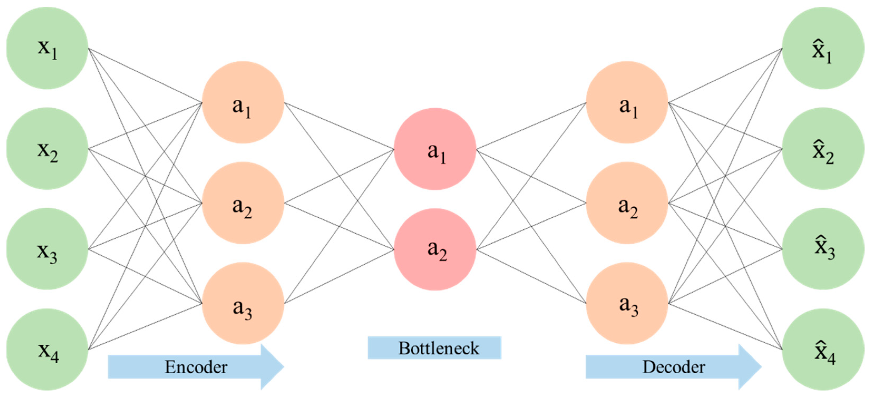
• The established literature reveals that the sequential learning approaches have a strong performance in time series prediction data. Inspired by their reasonable and accurate performances for prediction problems, for the first time, a novel hybrid network composed of an AE and BiLSTM is proposed for single-step forecasting of RE power generation.
• Short-term RES power production forecasting is very useful, and this information can improve the performance of existing energy systems. Furthermore, short-term forecasting of power allows for efficient integration, trading, storage unit management, and control systems of energy. Therefore, in this paper, we propose a model that has the ability to forecast short-term horizons for one-step RE forecasting.
• To confirm and verify the effectiveness of the proposed method, we conduct an extensive set of experiments on publicly available power generation datasets. We experimentally prove that the proposed method outperforms state-of-the-art methods by comparing it with competitive models including BiLSTM, CNN-BiLSTM, and an encoder–decoder (ED) via basic evaluation metrics such as mean absolute error (MAE), mean squared error (MSE), and root mean square error (RMSE), where the proposed AB-Net obtains the lowest error rate.

The remaining part of this paper is structured as follows: Briefly, the literature on RE forecasting is discussed in Section 2. Section 3 provides the detailed research methodology and its full overview. Section 4 discusses the experiments and visual representation of the results, while Section 5 concludes the paper along with further research directions.

2. Literature Review

In recent years, researchers have switched their attentions towards RESs for estimating power generation. These sources have been widely utilized for power generation due to the ease of their availability and renewable nature. One of the challenges in power production from RESs is its sustainability. Prediction of power generation from RESs mainly depends on environmental variables such as wind speed, wind direction, and weather conditions. These non-human controllable parameters make the prediction problem more challenging. Different types of prediction techniques have been utilized for estimating power generation from the renewable sources that are discussed in the following subsections.

2.1. Wind Power Generation

In the domain of wind power generation forecasting, different statistical, DL, and ML methods have traditionally been used. For instance, Liu et al. [24] proposed a combined model for short-term wind speed forecasting that utilized a multi-objective optimization algorithm to tackle wind speed issues such as nonlinearity, irregularity, and non-stationarity. Similarly, Sun et al. [25] introduced a hybrid approach by incorporating various techniques such as LSTM principle computing, secondary decomposition, and random forest to tackle issues related to wind energy generation such as sustainability and sanitation. Next, Hu et al. [26] proposed a stacked hierarchy of reservoirs which introduces the basic echo state network and DL framework for power production and consumption forecasting. Sharifzadeh et al. [27] conducted a study using an ANN, Gaussian process regression, and SVR for the prediction of future energy from wind resources. Similarly, Demolli et al. [28] used extreme GB (XGB) regression, SVR, and RF approaches for wind power energy forecasting using daily wind speed data. Li et al. [29] applied the least square SVM for short-term wind speed prediction, while Andrade et al. [30] presented a wind and solar power prediction model using the GB decision tree (DT) algorithm with feature engineering techniques. Moreover, Khosravi et al. [31] investigated the fuzzy inference system (FIS), SVR, and other ML approaches to forecast wind speed data for a power plant located in Brazil. Guoyang et al. [32] analyzed time series data of wind speed using the autoregressive moving and autoregressive integrated moving average approaches to predict wind power. Furthermore, Ding et al. [33] used the KF model for online prediction of wind speed and power generation for an efficient grid management system. Manero et al. [34] evaluated different DL approaches using wind speed time series data for the prediction of wind power generation. Khan et al. [35] combined DL and principal component analysis approaches for forecasting wind power using datasets of hourly, monthly, and yearly wind speed data. Eze et al. [36] introduced LSTM networks for the prediction of power generated at a wind power plant. Liu et al. [37] practiced wavelet packets along with other DL approaches for wind speed prediction, with outstanding results.

2.2. Solar Power Generation

Solar energy is a limitless RES that does not emit carbon or other greenhouse gases, since it does not need fuel or other resources. This property makes it one of the most ecofriendly energy generation technologies. In solar energy, radiation is considered to be an important parameter with different intervals of time scales. Different ML and DL approaches based on data-driven methods have been used for the purpose of effective management at solar power plants. For instance, Aslam et al. [38] analyzed different DL approaches for the prediction of solar radiation for one year ahead in intervals of hours and days through a recurrent neural network (RNN), GRU, LSTM, feedforward neural network (FFNN), and SVR. Next, Torres-Barrán et al. [39] utilized the methods of RF regression, GB regression, and XGB for the prediction of power generation from the renewable sources of solar and wind. Another group, Saloux et al. [40], investigated DT, SVM, and ANN for the prediction of the heating demand at a solar power plant, while Sun et al. [41] presented a CNN-based prediction approach for PV power generation. Torres et al. [42] proposed an FFNN to predict the day ahead electricity generated by PV solar systems, while Kamadinata et al. [43] forecasted the solar radiation from sky images using the ANN architecture. Similarly, Correa-Jullian et al. [44] explored the techniques of ANN, RNN, and LSTM and found these methods reliable for solar energy prediction. AlKandari et al. [45] used both ML and statistical methods for the prediction of future solar power generation in solar plants. Liu et al. [46] comparatively analyzed the SVM and copula-based nonlinear quantile regression (CNQR) approaches in terms of predicting solar radiation and proved the efficiency of CNQR over SVM.

2.3. Hydropower Generation

Among RESs, hydropower is also one of the most widely used power generation sources. Water sources are used for energy production due to their efficient characteristics, economic viability, and availability [47]. Different resources of water such as rivers and stored water are used for power generation purposes. Rainfall is also considered an important parameter affecting the power generation process [48]. Different types of prediction approaches have been presented for the better planning and management of hydropower plants [49]. For instance, Sapitang et al. [50] predicted the water level at a hydropower generation plant using the supervised ML approaches of Bayesian linear regression (LR), boosted DT regression, neural network regression, and decision forest regression. Similarly, Dehghani et al. [51] presented a promising approach using gray wolf optimization and an adaptive neuro-fuzzy inference system for hydropower generation prediction. Further, Zhang et al. [52] presented a multi-step hybrid approach of long-, medium-, and short-term Bayesian stochastic dynamic programming for the purpose of forecasting hydropower inflows. Hong et al. [53] forecasted rainfall with the hybrid approach of RNN and SVR along with the chaotic particle swarm optimization approach, while Wang et al. [54] presented a seasonal decomposition-based least square SVR approach for power generation prediction in hydropower plants. Lansberry et al. [55] utilized the genetic algorithm approach for optimization of the gains of governors that are plant parameters of the conduit constant and load self-legalization at a hydropower plant. Similarly, the authors in [56] used wavelet transform and SVR to predict tidal current speed and direction at a tidal power generation plant. Safari et al. [57] predicted tidal current speed and direction using least square SVR and ensemble empirical mode decomposition. Ozbas et al. [58] predicted hydrogen production through biomass gasification using ML-based approaches of LR, SVM regression, k-NN regression, and DT regression.

3. Methodology

This section discusses the proposed framework for power generation prediction. First, we discuss the data acquisition and preprocessing steps. Then, the technical details of the proposed AB-Net architecture are presented, and, finally, the model evaluation strategy is explained. The overall framework of the proposed system is shown in Figure 1.

3.1. Data Acquisition and Preprocessing

In this section, we discuss the data acquisition and preprocessing steps in detail. Power is generated from different RESs such as wind, hydro, solar, geothermal, tidal, and biomass. The generated power from renewable sources is provided to consumers through a power distribution system such as a smart grid. In the proposed method, solar and wind power generation data are considered. Detailed descriptions of each dataset such as location, time, samples, duration, interval, and other attributes are presented in Table 1 (Section 4.1). Several smart sensors are installed in smart grids that measure the power generation and consumption information, and they keep records for future analysis. These previous data such as power generation and consumption are utilized for training ML and DL models for future power generation forecasting and consumption prediction. During the acquisition of data, there are some uncertainties in the data such as noise and missing values. To remove these abnormalities, preprocessing techniques are applied. The moving average filter is an important technique that is utilized to smooth data and make them appropriate for model training. For handling missing values, the substitution method can be applied, where missing values are filled with previous time values. ML and DL models learn to map the input data to the output data [59]. There are multiple variables in input data that have different distributions and scale ranges. The difference between the scale and distribution of the input variables makes it difficult to model a particular problem. Hence, DL models learn huge values for weights when the input variable values are large and the values are in different ranges. As a result, the model becomes unstable and yields a poor performance. Similarly, a model with large values for weights has a higher generalization error and suffers from a poor performance throughout the learning. Furthermore, a large difference in output variable values makes the learning process unstable and results in a large error gradient. Therefore, it is very important to scale the input and output data before training ML and DL models. To tackle the above-mentioned problems, the input and output variable data can be normalized to a range of 0 and 1.

3.2. Proposed Network for Power Generation

This section discusses the proposed AB-Net framework, which is a hybrid network of an AE and BiLSTM. Then, various sequential models such as RNN, LSTM, BiLSTM, and an autoencoder are discussed in the following subsections.

3.2.1. Recurrent Neural Network

RNNs are an important type of DNN which deals with sequential data using the internal memory concept and loops. Figure 2a shows the basic structure of an RNN that is similar to the architecture of LSTM, while Figure 2b illustrates the unfolded structure. The calculation process of a hidden layer state is presented in Equation (1). The hidden state h_t of a hidden layer is modified and retained on the basis of the previous hidden state h_t−1 and the layer input x_t at every time interval t.

$$h_t={\sigma }_h\left(W_{xh}{X}_t+W_{hh}{h}_{t-1}+b_h\right)$$

(1)

$$y_t={\sigma }_y\left(W_{hy}{h}_t+b_y\right)$$

(2)

In Equation (1),${\sigma }_h$ is the activation function, $W_{xh}$ is the weight matrix for the input to the hidden layer, $W_{hh}$ is successive hidden states’ weight matrix, and $b_h$ is the hidden layer bias vector to produce the hidden state. The output of the network is shown in Equation (2), where ${\sigma }_y$ is the output layer activation function, and $W_{hy}$ is the weight matrix for the hidden layer to the output layer, while the output layer bias vector is represented by $b_y$. In nonlinear time series problems, RNNs have shown a good performance compared to traditional ML methods. However, general RNNs have some problems during backpropagation such as exploding gradients and vanishing gradients due to which these sequential models become incapable of learning long-term dependencies and longtime lags.

3.2.2. Long Short-Term Memory

RNNs suffer from vanishing and exploding gradient problems; therefore, to handle these issues, the architecture of LSTM has been introduced, which is well known for its good performance on sequential problems with long-term dependencies [60]. The hidden layer of LSTM, which is also called the LSTM cell, makes it different from the general RNN architecture [61]. Figure 3a shows the hidden layer of LSTM, where $x_t$ is the input of the cell at time t, and $h_t$ is the output. During weight updating and training, the hidden layer of LSTM also considers different cell states including the input $C_t$, output ${\tilde{C}}_t$, and previous output $C_{t-1}$. The gate concept is present in LSTM compared to general RNNs due to which LSTM is capable of learning useful information from long-term as well as short-term dependencies. LSTM includes three types of gates: input, forget, and output gates, which make it an effective and scalable model for various sequence-based tasks. In Figure 3a, for time t, the input gate of the LSTM cell is represented by $i_t$ and the forget gate by $f_t$, while the output gate is represented by $o_t$. Equations (3)–(6) are used to calculate the gates of a cell [62].

$$f_t={\sigma }_g\left(W_f{X}_t+U_f{h}_{t-1}+b_f\right)$$

(3)

$$i_t={\sigma }_g\left(W_i{X}_t+U_i{h}_{t-1}+b_i\right)$$

(4)

$$o_t={\sigma }_g\left(W_o{X}_t+U_o{h}_{t-1}+b_o\right)$$

(5)

$${\tilde{C}}_t=tanh\left(W_c{X}_c+U_c{h}_{t-1}+b_c\right)$$

(6)

In the above equations, ${\sigma }_g$ is the activation function for each gate which is normally a sigmoid function, while the hyperbolic tangent function is represented by $tanh$. Weight matrices are represented by $W_f$,$W_i$, and $W_o$ for mapping from the cell input to the LSTM gates, while $W_c$ is the weight matrix for mapping the cell input to the input cell state. Similarly, for connecting the prior hidden layer output state to the gates and the input cell state, weight matrices are represented by $U_f$,$U_i$, $U_o$, and $U_c$. The bias vectors are represented by $b_f$, $b_i$, $b_o$, and $b_c$ in each equation. At time interval t, the layer output $h_t$ and cell output state $C_t$ can be calculated using Equations (7) and (8):

$$C_t=f_t\ast C_{t-1}+i_t\ast {\tilde{C}}_t$$

(7)

$$h_t=o_t\ast tanh\left(C_t\right)$$

(8)

3.2.3. Bidirectional LSTM

The bidirectional RNN and BiLSTM ideas are similar, which involve the processing of sequential data with separate hidden layers in both directions, i.e., forward and backward [63]. These two hidden layers are connected to the same output layer in a BiLSTM network, and it is proved that these bidirectional networks are considerably better than unidirectional models in many domains such as speech classification and gene sequence classification. Figure 3b shows the unfolded structure of BiLSTM, which contains the forward and backward LSTM layers. The output sequence of the forward layer $\overrightarrow{h}$ is repeatedly calculated from time T − n to time T − 1, utilizing inputs in a positive sequence. Similarly, by means of reversed inputs from T − n to T − 1, the output sequence of the backward layer $\overleftarrow{h}$ is iteratively calculated. The bidirectional layer produces an output vector where every element is calculated using the following Equation (9):

$$y_t=\sigma \left({\overrightarrow{h}}_t,{\overleftarrow{h}}_t\right)$$

(9)

To combine the forward and backward layer output sequences, the function $\sigma$ is used. This function can have different purposes such as summation, average, concatenation, or multiplication.

3.2.4. Bidirectional Autoencoder

An AE performs the task of learning the compact representation of data using an unsupervised learning approach. In this technique, a neural network architecture is designed in such a way that imposes a compressed information representation of the original input data. Figure 4 shows that unlabeled data can be framed as a supervised learning task with the reconstruction of the original input data. There are three types of layers in an AE, which are the input, hidden, and output layers, where the hidden layers learn to encode the data, while the output layers reconstruct the original data from the encoded data [64]. An AE is trained in order to reduce the reconstruction error, which is the difference between the reconstructed data and original input data. The important attribute in the AE architecture design is the bottleneck, which is utilized to obtain the compressed form of the original input data. An AE simply learns to memorize the input data by passing the data through the model with the presence of bottleneck information. The bottleneck is responsible for restraining the required information by traversing the whole architecture, forcing the original input data into a compressed representation. A small number of nodes are maintained in the hidden layer of our network architecture due to which the information flow is also reduced through the network. The AE is trained according to the reconstruction error and tries to learn the key attributes from the original input data, which is called data encoding, and then it tries to reconstruct the real original data from the encoded data, which is called data decoding. A BiLSTM-based ED structure can be used to implement a BiLSTM-based AE for time series data. A BiLSTM-based ED is constructed for sequential input data in such a way that it can read the input data properly, encode it, and finally reconstruct it. The efficiency of the architecture is then computed from its capability to reconstruct the original input time series data. During unsupervised learning, when the model obtains the preferred accuracy, the encoder part of the model is used to encode the input data to a fixed length vector, while the decoder part of the model is removed.

3.3. Model Evaluation

In this work, an ablation study was conducted using four different sequential models on two publicly available power generation datasets. In the proposed AB-Net model, first, a BiLSTM autoencoder is trained, then its decoder part is removed, and the encoder part is used for extracting the meaningful features from the data. Finally, the extracted features are passed through another BiLSTM network for one-step forecasting of power generation. All the forecasting methods were evaluated using basic error metrics that are presented in Equations (10)–(12) and visual graphs. For instance, $y_i^{~}$ shows variable values for n number of predictions that are samples from the power generation, while $y_i$ shows the predicted/observed numbers. The MSE calculates the average of squared error, showing the difference between the estimated and observed values. Similarly, the RMSE is the square root of the value obtained from the MSE. The details of the ablation study are presented in the Experimental Result section.

$$MSE=\frac{1}{n}{\displaystyle \sum }_{i=1}^n{\left(y_i-y_i^{~}\right)}^2$$

(10)

$$RMSE=\sqrt{\frac{1}{n}{\displaystyle \sum }_{i=1}^n{\left(y_i-y_i^{~}\right)}^2}$$

(11)

$$MAE=\frac{1}{n}{\displaystyle \sum }_{i=1}^n\left|y_i-y_i^{~}\right|$$

(12)

System Settings and Hyperparameters

The sequential models used for power generation forecasting were implemented in Python (version 3.8.5) with a popular DL framework (Keras) with Tensorflow at the backend. Each model was trained up to 100 epochs on each dataset with the Adam optimizer, with a learning rate of 0.001, and a batch size of 16. In the BiLSTM network, two BiLSTM layers with 200 and 100 neurons are used for the first and second layers, respectively, followed by a fully connected layer with 50 neurons. Similarly, in the CNN-BiLSTM network, two layers of a one-dimensional CNN are used with a 1 × 3 filter size, while 128 and 256 filters are utilized in the first and second layers, respectively, followed by a max pooling layer. After the CNN layers, two BiLSTM layers having 200 and 100 neurons are used, followed by a fully connected layer with 50 neurons. Furthermore, the encoder part of the ED model has two BiLSTM layers with 200 and 100 neurons in the first and second layers, respectively, while the decoder part also comprises two BiLSTM layers with 100 and 200 neurons. After the decoder part, there is one fully connected layer with 50 neurons. The proposed model is a hybrid connection of two networks that uses the encoder part of the AE for feature extraction and passes the features to the BiLSM layers for decoding. The encoder part of the AE in the proposed model contains two BiLSM layers with 200 and 100 neurons. After that, two layers of BiLSM are used, having 200 and 100 neurons, followed by a fully connected layer with 50 neurons.

4. Experimental Results

This section thoroughly explains the experiments performed for power generation forecasting using publicly available datasets with the hold-out method to evaluate the performance of the proposed method. We used 70% and 30% of the data for training and testing, respectively, which is a standard data splitting procedure. Next, for classification purposes, model validation was performed via accuracy, recall, and precision. However, time series forecasting is a regression problem; therefore, basic error metrics such as the MSE, RMSE, and MAE were assessed, which are widely used to validate and verify the effectiveness of regression problems.

4.1. Datasets

To verify and evaluate the performance of the proposed method, two publicly available datasets, namely, a solar dataset [65] and a wind dataset [66], were used. The description of each dataset is presented in Table 1.

Table 1. Detailed description of each dataset along with its parameters and units.

Dataset	Parameters	Values
Wind Dataset [66]	Plant Max Output	16 MW
	Max Wind Speed	23.0352
	Max Wind Direction	359.3794 degrees
	Max Temperature	35.9660 degrees Celsius
	Max Air Pressure	8.5927 × 104 Pas
	Max Air Density	1.0980 Kg/m3
	Longitude	−104.258
	Latitude	35.00168
	Duration	(1 Year) 2012
	Time Interval	5 min
	Totals Points	105,121
Solar Dataset [65]	Plant Max Output	2610 kW
	Plant Capacity	3026 kW
	Max Inclined Irradiance	999.96
	Max Surface Temperature	49.78
	Max Surrounding Temperature	125.60
	Duration	3 years, 10 months (2015 to 2018)
	Time Interval	1 h
	Totals Points	17,252

Table 1. Detailed description of each dataset along with its parameters and units.

Dataset	Parameters	Values
Wind Dataset [66]	Plant Max Output	16 MW
	Max Wind Speed	23.0352
	Max Wind Direction	359.3794 degrees
	Max Temperature	35.9660 degrees Celsius
	Max Air Pressure	8.5927 × 104 Pas
	Max Air Density	1.0980 Kg/m3
	Longitude	−104.258
	Latitude	35.00168
	Duration	(1 Year) 2012
	Time Interval	5 min
	Totals Points	105,121
Solar Dataset [65]	Plant Max Output	2610 kW
	Plant Capacity	3026 kW
	Max Inclined Irradiance	999.96
	Max Surface Temperature	49.78
	Max Surrounding Temperature	125.60
	Duration	3 years, 10 months (2015 to 2018)
	Time Interval	1 h
	Totals Points	17,252

4.1.1. Solar Dataset

The solar dataset was obtained from [65] and was collected at a solar plant located at the stadium of the Yeongam F1. These data cover three years and ten months (i.e., January 2015 to October 2018). The input variables in the dataset are inclined irradiance, surrounding temperature, and surface temperature, while the output power is considered as a predicted variable.

4.1.2. Wind Dataset

This dataset was obtained from NREL [66] and was gathered in New Kirk. The wind dataset consists of power, wind speed, wind direction, surface air pressure, air temperature, and air density. In this dataset, five variables such as wind direction, air temperature, wind speed, air density, and surface air pressure are considered as input variables, while the power is considered to be forecasted.

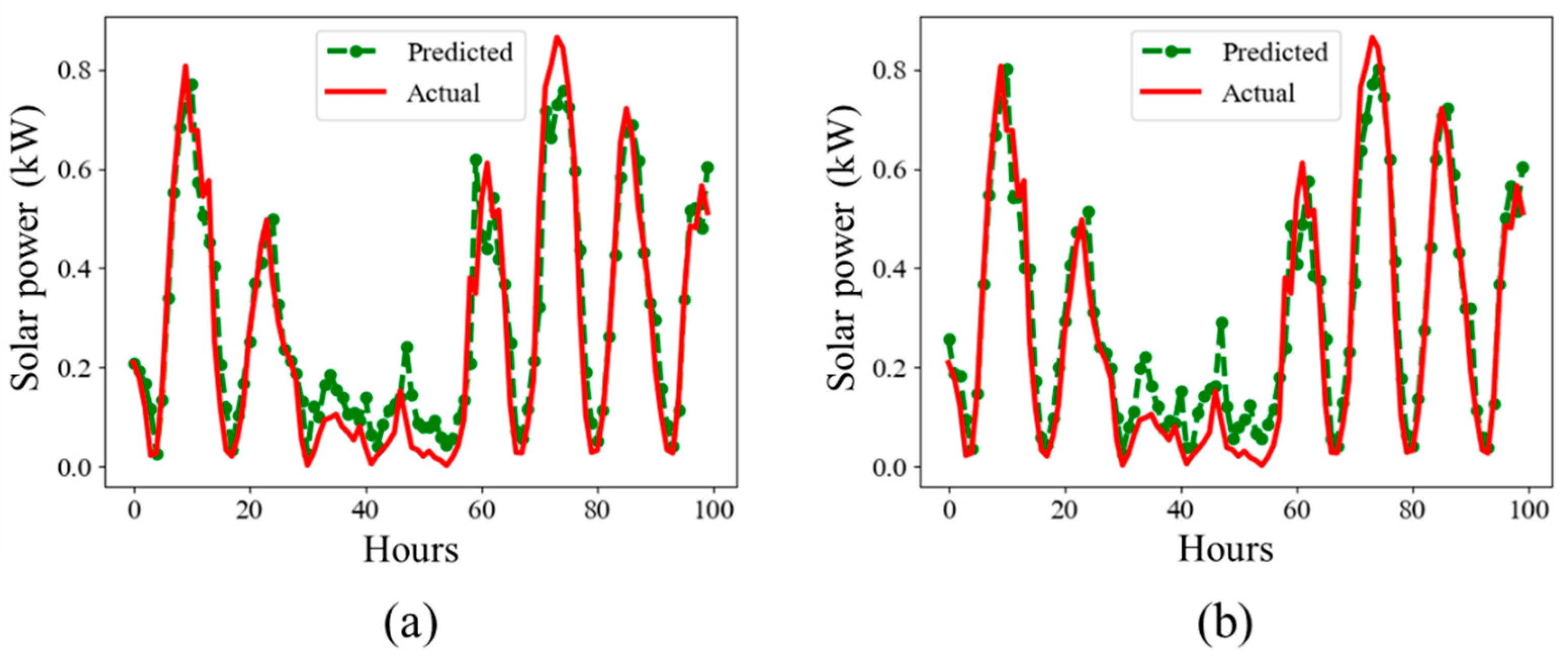
4.2. Results on Solar Dataset

This section discusses the results obtained over state-of-the-art techniques that include the most popular competitive DL networks such as BiLSTM, CNN-BiLSTM, ED, and AB-Net.

There are several studies that have used different DL approaches for forecasting purposes. The RNN architecture is one of the most employed techniques for forecasting problems, which is capable of remembering the preceding input data to learn the weights of the network. Several variants of the RNN architecture such as LSTM and BiLSTM have been used that have improved the network’s ability to preserve the network states by capturing the long-term sequential dependencies. Initially, LSTM was formed to extend the memory state in RNNs and to enable them to deal with long-term dependencies. Similarly, another form is BiLSTM, where the proceeding input sequences are learned in both the forward and backward directions. In BiLSTM, several layers are stacked to capture the complex features in time series. In the experiments, we firstly analyzed the results obtained over BiLSTM by using its predefined settings. The two layers are stacked together to process the input data, where each layer performs its operations in the reverse direction. The results obtained from BiLSTM are combined in the final layer to produce the final prediction/forecast. BiLSTM was found to be effective in the literature. The MSE value obtained by BiLSTM on the solar dataset was 0.0112. The value is presented in

Table 2. Results obtained for different models on solar data via ablation study.

Method	MSE	RMSE	MAE
BiLSTM	0.0112	0.1060	0.0778
CNN-BiLSTM	0.0111	0.1055	0.0748
ED	0.0107	0.1036	0.0747
AB-Net	0.0106	0.1028	0.0743

, where the RMSE and MAE are also shown. The forecasting graph obtained over BiLSTM is presented in Figure 5a. Next, the experiments were performed on the hybrid network where CNN and BiLSTM are combined to extract the most important and discriminative features. In this network, the features from multivariate data are extracted through the CNN layers which contain the most important details about the sequential series data. The features obtained through the CNN are forward propagated into BiLSTM to learn them for forecasting purposes. The value obtained for the MSE on the solar dataset was 0.0111, while the other metric values such as the RMSE and MAE are presented in Table 2. The forecasting graph obtained over CNN-BiLSTM is presented in Figure 5b.

Next, the ED model was applied, which is also a technique of using BiLSTM for sequence-to-sequence forecasting problems. This technique involves two BiLSTM networks, where one network encodes the sequence, known as an encoder, while the other decodes the input sequence into a target, called a decoder. The encoder takes a single element from the input sequence at every time step by processing it. It collects the information and forward propagates it. The encoder produces an internal state that contains the information about the entire sequence that helps the decoder to carry out accurate forecasting. Finally, the decoder provides the final prediction at each time step. The MSE value obtained with the ED on the solar dataset was 0.0107. The value is presented in Table 2, where the RMSE and MAE are also presented. The forecasting graph obtained over the ED is presented in Figure 6a.

The proposed method is a hybrid connection of an AE and BiLSTM, rendering the network more capable of extracting the most important and hierarchical features from the multivariate data. The initial part of the network consists of an AE that takes the input sequence and analyzes it for detailed information collection. After this step, once the information from the AE part is collected, this information is forward propagated into the BiLSTM for final forecasting. In traditional time series data problems, the AE is usually formed by stacking simple LSTM layers that are not effective in encoding long-term dependencies. However, in the proposed method, we create the AE part from the BiLSTM. The output from the AE is forward fed into the BiLSTM to learn the sequence and provide the final prediction/forecast. The first input layer is a BiLSTM that is followed by another BiLSTM layer, which has a small size. The output taken from the encoder part of the AE is fed into the repeat vector, which is a single vector that reshapes it in our BiLSTM network. The value of the MSE obtained on the solar data was 0.0106. The value is presented in Table 2, where the RMSE and MAE are also presented. The forecasting graph obtained over AB-Net is presented in Figure 6b.

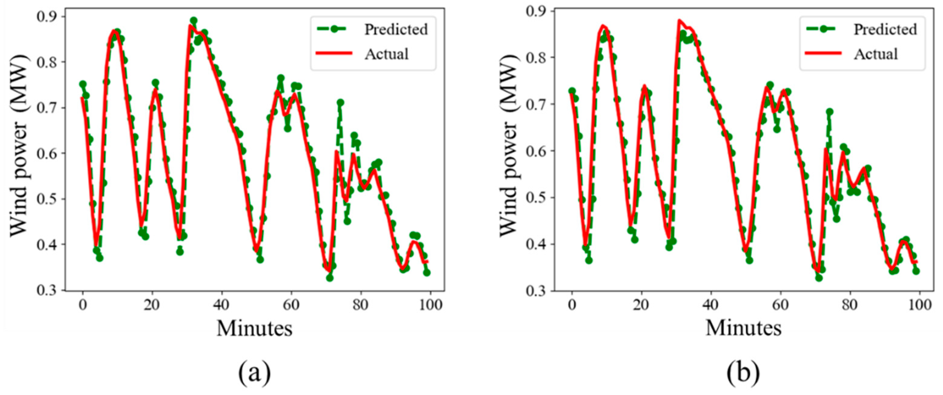
4.3. Results on Wind Dataset

This section thoroughly explains the results obtained on the wind dataset. Similar to the solar dataset, we practiced the same strategy that was previously applied for the ablation study.

Firstly, the BiLSTM was applied to study its performance on the wind dataset, where we examined that the BiLSTM has a good performance compared to its results on the solar dataset. In fact, the wind blows for a constant time, and the air turbines continuously operate for 24 h, while the solar panel only works in the daytime where sunlight radiation occurs in a specific period. Therefore, some values in this duration are not recorded. The obtained MSE value by the BiLSTM on the wind dataset was 0.0005, while the RMSE and MAE were 0.0219 and 0.0142, respectively. The forecasting graph obtained over BiLSTM is presented in Figure 7a. The hybrid connection of CNN and BiLSTM was also evaluated on the wind dataset, and it was found to perform better than the results obtained on the solar dataset due to the same previously stated reason. However, its results on the wind dataset are better than the simple BiLSTM, where the obtained MSE value was 0.0005, while the RMSE and MAE values were 0.0216 and 0.0133, respectively. The forecasting graph obtained over CNN-BiLSTM is presented in Figure 7b.

The ED that was formed by the BiLSTM variants was also evaluated on the wind dataset and obtained promising results. The architectural details of ED have been previously discussed. The ED performed better than BiLSTM and CNN-BiLSTM by obtaining a 0.0005 MSE on the wind dataset. The RMSE and MAE values were 0.0198 and 0.0130, respectively. The forecasting graph obtained over ED is presented in Figure 8a. Finally, the proposed AB-Net architecture was evaluated on the wind dataset, which beats all the previously practiced networks on the wind dataset. The network settings of the proposed AB-Net have already been explained in the previous section, and its further details are out of the scope of this paper. The obtained MSE of the proposed method on the wind dataset was 0.0004, while the RMSE and MAE values were 0.0189 and 0.0109, respectively, as shown in

Table 3. Results obtained for different models on wind data via ablation study.

Method	MSE	RMSE	MAE
BiLSTM	0.0005	0.0219	0.0142
CNN-BiLSTM	0.0005	0.0216	0.0133
ED	0.0005	0.0198	0.0130
AB-Net	0.0004	0.0189	0.0109

. The forecasting graph obtained over AB-Net is presented in Figure 8b.

4.4. Assessment with State of the Art

In this section, we compare the proposed method with recent research carried out for power generation forecasting. Both the solar and wind datasets were considered for the comparative study. The comparison was performed with the most recent method [67], where a mode-adaptive ANN algorithm is proposed via Spearman’s ranking order and population-based algorithms. They evaluate different models such as advanced particle swarm optimization (APSO) and the fine-tuning metaheuristic algorithm (FTMA). We considered their most outstanding results for the comparison, which were obtained using FTMA, in their case. The MSE values obtained by FTMA on the solar dataset and wind dataset were 0.0207 and 0.4944, while the RMSE was 0.1438 and 0.7031, respectively. Finally, we pose the results of the proposed method on the solar dataset where the obtained MSE, RMSE, and MAE were 0.0106, 0.1028, and 0.0743, respectively, while the MSE, RMSE, and MAE for the wind dataset were 0.0004, 0.0189, and 0.0109, respectively. Comparative results are shown in Figure 9a,b for both datasets.

5. Conclusions

To mitigate climate change and global warming impacts, RE usage is significantly increasing on a daily basis. A certain amount of power has been generated by different RESs in recent decades. The power generated through these plants is used by consumers for different applications. However, the power produced needs to be predicted so that an exact amount of power is produced in the future. To forecast this problem, several techniques have come into the foreground, where the majority of these methods are based on traditional learning techniques. To this purpose, we developed a novel architecture that creates a hybrid connection between an AE and a BiLSTM network. Initially, the data are cleaned through a refinement step in the preprocessing step, and their refined sequence is passed into the AE for feature collection. The obtained features from the AE are fed into the BiLSTM for final forecasting. The proposed approach is capable of learning a compressed representation from the sequential input data and of forecasting RES power accurately. The proposed method is helpful to avoid extra production of power energy and its wastage. The smart grid and the consumer side will smoothly cooperate following the proposed algorithm. Further, using publicly available datasets, the proposed method’s performance was shown to be higher than state-of-the-art techniques.

In the future, we aim to consider different scenarios for power energy generation and its consumption by residential areas, industries, and the commercial side for proper energy management. Moreover, lightweight models will be investigated for their deployment as prediction models over resource-constrained devices by reducing the computation and cost.

References

1. Mayer, M.J.; Szilágyi, A.; Gróf, G. Environmental and economic multi-objective optimization of a household level hybrid renewable energy system by genetic algorithm. Appl. Energy 2020, 269, 115058. [Google Scholar] [CrossRef]
2. Hu, X.; Zou, Y.; Yang, Y. Greener plug-in hybrid electric vehicles incorporating renewable energy and rapid system optimization. Energy 2016, 111, 971–980. [Google Scholar] [CrossRef]
3. Xiong, L.; Li, P.; Wang, Z.; Wang, J. Multi-agent based multi objective renewable energy management for diversified community power consumers. Appl. Energy 2020, 259, 114140. [Google Scholar] [CrossRef]
4. Khan, N.; Ullah FU, M.; Ullah, A.; Lee, M.Y.; Baik, S.W. Batteries state of health estimation via efficient neural networks with multiple channel charging profiles. IEEE Access 2020, 9, 7797–7813. [Google Scholar] [CrossRef]
5. Kang, J.N.; Wei, Y.M.; Liu, L.C.; Han, R.; Yu, B.Y.; Wang, J.W. Energy systems for climate change mitigation: A systematic review. Appl. Energy 2020, 263, 114602. [Google Scholar] [CrossRef]
6. Pillot, B.; Muselli, M.; Poggi, P.; Dias, J.B. Historical trends in global energy policy and renewable power system issues in Sub-Saharan Africa: The case of solar PV. Energy Policy 2019, 127, 113–124. [Google Scholar] [CrossRef]
7. Javed, M.S.; Zhong, D.; Ma, T.; Song, A.; Ahmed, S. Hybrid pumped hydro and battery storage for renewable energy based power supply system. Appl. Energy 2020, 257, 114026. [Google Scholar] [CrossRef]
8. Nam, K.; Hwangbo, S.; Yoo, C. A deep learning-based forecasting model for renewable energy scenarios to guide sustainable energy policy: A case study of Korea. Renew. Sustain. Energy Rev. 2020, 122, 109725. [Google Scholar] [CrossRef]
9. Ahmad, T.; Zhang, H.; Yan, B. A review on renewable energy and electricity requirement forecasting models for smart grid and buildings. Sustain. Cities Soc. 2020, 55, 102052. [Google Scholar] [CrossRef]
10. Aslam, S.; Herodotou, H.; Mohsin, S.M.; Javaid, N.; Ashraf, N.; Aslam, S. A survey on deep learning methods for power load and renewable energy forecasting in smart microgrids. Renew. Sustain. Energy Rev. 2021, 144, 110992. [Google Scholar] [CrossRef]
11. Hodge, B.M.; Martinez-Anido, C.B.; Wang, Q.; Chartan, E.; Florita, A.; Kiviluoma, J. The combined value of wind and solar power forecasting improvements and electricity storage. Appl. Energy 2018, 214, 1–15. [Google Scholar] [CrossRef]
12. Sajjad, M.; Khan, S.U.; Khan, N.; Haq, I.U.; Ullah, A.; Lee, M.Y.; Baik, S.W. Towards efficient building designing: Heating and cooling load prediction via multi-output model. Sensors 2020, 20, 6419. [Google Scholar] [CrossRef]
13. Wang, H.; Lei, Z.; Zhang, X.; Zhou, B.; Peng, J.A. review of deep learning for renewable energy forecasting. Energy Convers. Manag. 2019, 198, 111799. [Google Scholar] [CrossRef]
14. Singh, S.; Mohapatra, A. Repeated wavelet transform based ARIMA model for very short-term wind speed forecasting. Renew. Energy 2019, 136, 758–768. [Google Scholar]
15. Yang, D. On post-processing day-ahead NWP forecasts using Kalman filtering. Sol. Energy 2019, 182, 179–181. [Google Scholar] [CrossRef]
16. Wang, Y.; Wang, H.; Srinivasan, D.; Hu, Q. Robust functional regression for wind speed forecasting based on Sparse Bayesian learning. Renew. Energy 2019, 132, 43–60. [Google Scholar] [CrossRef]
17. Li, G.; Xie, S.; Wang, B.; Xin, J.; Li, Y.; Du, S. Photovoltaic power forecasting with a hybrid deep learning approach. IEEE Access 2020, 8, 175871–175880. [Google Scholar] [CrossRef]
18. Haq, I.U.; Ullah, A.; Khan, S.U.; Khan, N.; Lee, M.Y.; Rho, S.; Baik, S.W. Sequential learning-based energy consumption prediction model for residential and commercial sectors. Mathematics 2021, 9, 605. [Google Scholar] [CrossRef]
19. Khan, N.; Haq, I.U.; Khan, S.U.; Rho, S.; Lee, M.Y.; Baik, S.W. DB-Net: A novel dilated CNN based multi-step forecasting model for power consumption in integrated local energy systems. Int. J. Electr. Power Energy Syst. 2021, 133, 107023. [Google Scholar] [CrossRef]
20. Gensler, A.; Henze, J.; Sick, B.; Raabe, N. Deep Learning for solar power forecasting—An approach using AutoEncoder and LSTM Neural Networks. In Proceedings of the 2016 IEEE International Conference on Systems, Man, and Cybernetics (SMC), Budapest, Hungary, 9–12 October 2016; IEEE: Piscataway, NJ, USA, 2016. [Google Scholar]
21. Maciel, J.N.; Ledesma JJ, G.; Junior, O.H.A. Forecasting Solar Power Output Generation: A Systematic Review with the Proknow-C. IEEE Lat. Am. Trans. 2021, 19, 612–624. [Google Scholar] [CrossRef]
22. Barbieri, F.; Rajakaruna, S.; Ghosh, A. Very short-term photovoltaic power forecasting with cloud modeling: A review. Renew. Sustain. Energy Rev. 2017, 75, 242–263. [Google Scholar] [CrossRef] [Green Version]
23. Ferrero Bermejo, J.; Gomez Fernandez, J.F.; Olivencia Polo, F.; Crespo Marquez, A. A review of the use of artificial neural network models for energy and reliability prediction. A study of the solar PV, hydraulic and wind energy sources. Appl. Sci. 2019, 9, 1844. [Google Scholar]
24. Liu, Z.; Jiang, P.; Zhang, L.; Niu, X.A. combined forecasting model for time series: Application to short-term wind speed forecasting. Appl. Energy 2020, 259, 114137. [Google Scholar] [CrossRef]
25. Sun, H. Hybrid model with secondary decomposition, randomforest algorithm, clustering analysis and long short memory network principal computing for short-term wind power forecasting on multiple scales. Energy 2021, 221, 119848. [Google Scholar] [CrossRef]
26. Hu, H.; Wang, L.; Lv, S.X. Forecasting energy consumption and wind power generation using deep echo state network. Renew. Energy 2020, 154, 598–613. [Google Scholar] [CrossRef]
27. Sharifzadeh, M.; Sikinioti-Lock, A.; Shah, N. Machine-learning methods for integrated renewable power generation: A comparative study of artificial neural networks, support vector regression, and Gaussian Process Regression. Renew. Sustain. Energy Rev. 2019, 108, 513–538. [Google Scholar] [CrossRef]
28. Demolli, H.; Dokuz, A.S.; Ecemis, A.; Gokcek, M. Wind power forecasting based on daily wind speed data using machine learning algorithms. Energy Convers. Manag. 2019, 198, 111823. [Google Scholar] [CrossRef]
29. Li, Y.; Yang, P.; Wang, H. Short-term wind speed forecasting based on improved ant colony algorithm for LSSVM. Clust. Comput. 2019, 22, 11575–11581. [Google Scholar] [CrossRef]
30. Andrade, J.R.; Bessa, R.J. Improving renewable energy forecasting with a grid of numerical weather predictions. IEEE Trans. Sustain. Energy 2017, 8, 1571–1580. [Google Scholar] [CrossRef] [Green Version]
31. Khosravi, A.; Machado, L.; Nunes, R. Time-series prediction of wind speed using machine learning algorithms: A case study Osorio wind farm, Brazil. Appl. Energy 2018, 224, 550–566. [Google Scholar] [CrossRef]
32. Guoyang, W.; Yang, X.; Shasha, W. Discussion about short-term forecast of wind speed on wind farm. Jilin Electr. Power 2005, 181, 21–24. [Google Scholar]
33. Ding, M.; Zhang, L.J.; Wu, Y.C. Wind speed forecast model for wind farms based on time series analysis. Electr. Power Autom. Equip. 2005, 25, 32–34. [Google Scholar]
34. Manero, J.; Béjar, J.; Cortés, U. “Dust in the wind…”, deep learning application to wind energy time series forecasting. Energies 2019, 12, 2385. [Google Scholar]
35. Khan, M.; Liu, T.; Ullah, F. A new hybrid approach to forecast wind power for large scale wind turbine data using deep learning with TensorFlow framework and principal component analysis. Energies 2019, 12, 2229. [Google Scholar] [CrossRef] [Green Version]
36. Eze, E.C.; Chatwin, C.R. Enhanced recurrent neural network for short-term wind farm power output prediction. J. Appl. Sci. 2019, 5, 28–35. [Google Scholar]
37. Liu, H.; Mi, X.; Li, Y. Smart deep learning based wind speed prediction model using wavelet packet decomposition, convolutional neural network and convolutional long short term memory network. Energy Convers. Manag. 2018, 166, 120–131. [Google Scholar] [CrossRef]
38. Aslam, M.; Lee, J.M.; Kim, H.S.; Lee, S.J.; Hong, S. Deep learning models for long-term solar radiation forecasting considering microgrid installation: A comparative study. Energies 2020, 13, 147. [Google Scholar] [CrossRef] [Green Version]
39. Torres-Barrán, A.; Alonso, Á.; Dorronsoro, J.R. Regression tree ensembles for wind energy and solar radiation prediction. Neurocomputing 2019, 326, 151–160. [Google Scholar] [CrossRef]
40. Saloux, E.; Candanedo, J.A. Forecasting district heating demand using machine learning algorithms. Energy Procedia 2018, 149, 59–68. [Google Scholar] [CrossRef]
41. Sun, Y.; Venugopal, V.; Brandt, A.R. Short-term solar power forecast with deep learning: Exploring optimal input and output configuration. Sol. Energy 2019, 188, 730–741. [Google Scholar] [CrossRef]
42. Torres, J.F.; Troncoso, A.; Koprinska, I.; Wang, Z.; Martínez-Álvarez, F. Big data solar power forecasting based on deep learning and multiple data sources. Expert Syst. 2019, 36, e12394. [Google Scholar] [CrossRef]
43. Kamadinata, J.O.; Ken, T.L.; Suwa, T. Sky image-based solar irradiance prediction methodologies using artificial neural networks. Renew. Energy 2019, 134, 837–845. [Google Scholar] [CrossRef]
44. Correa-Jullian, C.; Cardemil, J.M.; Droguett, E.L.; Behzad, M. Assessment of Deep Learning techniques for Prognosis of solar thermal systems. Renew. Energy 2020, 145, 2178–2191. [Google Scholar] [CrossRef]
45. AlKandari, M.; Ahmad, I. Solar power generation forecasting using ensemble approach based on deep learning and statistical methods. Appl. Comput. Inform. 2020. [Google Scholar] [CrossRef]
46. Liu, Y.; Zhou, Y.; Chen, Y.; Wang, D.; Wang, Y.; Zhu, Y. Comparison of support vector machine and copula-based nonlinear quantile regression for estimating the daily diffuse solar radiation: A case study in China. Renew. Energy 2020, 146, 1101–1112. [Google Scholar] [CrossRef]
47. Perera, K.S.; Aung, Z.; Woon, W.L. Machine learning techniques for supporting renewable energy generation and integration: A survey. In Proceedings of the International Workshop on Data Analytics for Renewable Energy Integration, Nancy, France, 19 September 2014; Springer: Cham, Switzerland, 2014. [Google Scholar]
48. Hernández, E.; Sanchez-Anguix, V.; Julian, V.; Palanca, J.; Duque, N. Rainfall prediction: A deep learning approach. In Proceedings of the International Conference on Hybrid. Artificial Intelligence Systems, Seville, Spain, 18–20 April 2016; Springer: Cham, Switzerland, 2016. [Google Scholar]
49. Ardabili, S.; Mosavi, A.; Dehghani, M.; Várkonyi-Kóczy, A.R. Deep learning and machine learning in hydrological processes climate change and earth systems a systematic review. In Proceedings of the International Conference on Global Research and Education, Balatonfüred, Hungary, 4–7 September 2019; Springer: Cham, Switzerland, 2019. [Google Scholar]
50. Sapitang, M.; Ridwan, W.M.; Faizal Kushiar, K.; Najah Ahmed, A.; El-Shafie, A. Machine Learning Application in Reservoir Water Level Forecasting for Sustainable Hydropower Generation Strategy. Sustainability 2020, 12, 6121. [Google Scholar] [CrossRef]
51. Dehghani, M.; Riahi-Madvar, H.; Hooshyaripor, F.; Mosavi, A.; Shamshirband, S.; Zavadskas, E.K.; Chau, K.W. Prediction of hydropower generation using grey wolf optimization adaptive neuro-fuzzy inference system. Energies 2019, 12, 289. [Google Scholar] [CrossRef] [Green Version]
52. Zhang, X.; Peng, Y.; Xu, W.; Wang, B. An optimal operation model for hydropower stations considering inflow forecasts with different lead-times. Water Resour. Manag. 2019, 33, 173–188. [Google Scholar] [CrossRef]
53. Hong, W.-C. Rainfall forecasting by technological machine learning models. Appl. Math. Comput. 2008, 200, 41–57. [Google Scholar] [CrossRef]
54. Wang, S.; Tang, L.; Yu, L. SD-LSSVR-based decomposition-and-ensemble methodology with application to hydropower consumption forecasting. In Proceedings of the 2011 Fourth International Joint Conference on Computational Sciences and Optimization, Kunming and Lijiang, China, 15–19 April 2011; IEEE: Piscataway, NJ, USA, 2011. [Google Scholar]
55. Lansberry, J.; Wozniak, L.; Goldberg, D.E. Optimal hydrogenerator governor tuning with a genetic algorithm. IEEE Trans. Energy Convers. 1992, 7, 623–630. [Google Scholar] [CrossRef]
56. Kavousi-Fard, A.; Su, W. A combined prognostic model based on machine learning for tidal current prediction. IEEE Trans. Geosci. Remote. Sens. 2017, 55, 3108–3114. [Google Scholar] [CrossRef]
57. Safari, N.; Ansari, O.A.; Zare, A.; Chung, C.Y. A novel decomposition-based localized short-term tidal current speed and direction prediction model. In Proceedings of the 2017 IEEE Power & Energy Society General Meeting, Chicago, IL, USA, 16–20 July 2017; IEEE: Piscataway, NJ, USA, 2017. [Google Scholar]
58. Ozbas, E.E.; Aksu, D.; Ongen, A.; Aydin, M.A.; Ozcan, H.K. Hydrogen production via biomass gasification, and modeling by supervised machine learning algorithms. Int. J. Hydrogen Energy 2019, 44, 17260–17268. [Google Scholar] [CrossRef]
59. Khan, N.; Ullah, A.; Haq, I.U.; Menon, V.G.; Baik, S.W. SD-Net: Understanding overcrowded scenes in real-time via an efficient dilated convolutional neural network. J. Real-Time Image Process. 2021, 18, 1729–1743. [Google Scholar] [CrossRef]
60. Peng, L.; Zhu, Q.; Lv, S.X.; Wang, L. Effective long short-term memory with fruit fly optimization algorithm for time series forecasting. Soft Comput. 2020, 24, 15059–15079. [Google Scholar] [CrossRef]
61. Lee, J.; Kim, H.; Kim, H. Commercial Vacancy Prediction Using LSTM Neural Networks. Sustainability 2021, 13, 5400. [Google Scholar] [CrossRef]
62. Ullah FU, M.; Khan, N.; Hussain, T.; Lee, M.Y.; Baik, S.W. Diving Deep into Short-Term Electricity Load Forecasting: Comparative Analysis and a Novel Framework. Mathematics 2021, 9, 611. [Google Scholar] [CrossRef]
63. Ishaq, M.; Kwon, S. Short-Term Energy Forecasting Framework Using an Ensemble Deep Learning Approach. IEEE Access 2021, 9, 94262–94271. [Google Scholar]
64. Jaseena, K.; Kovoor, B.C. A hybrid wind speed forecasting model using stacked autoencoder and LSTM. J. Renew. Sustain. Energy 2020, 12, 023302. [Google Scholar] [CrossRef] [Green Version]
65. DATA.GO.KR. Available online: https://www.data.go.kr/ (accessed on 5 April 2021).
66. NREL Wind Prospector. Available online: https://maps.nrel.gov/wind-prospector/?aL=sgVvMX%255Bv%255D%3Dt&bL=groad&cE=0&lR=0&mC=41.983994270935625%2C-98.173828125&zL=5 (accessed on 5 April 2021).
67. Zamee, A.M.; Won, D. Novel Mode Adaptive Artificial Neural Network for Dynamic Learning: Application in Renewable Energy Sources Power Generation Prediction. Energies 2020, 13, 6405. [Google Scholar] [CrossRef]
Figure 1. Overall framework of the proposed architecture. In step 1, the power generation data are acquired, which are further preprocessed in step 2. In step 3, the features are extracted and passed through the BiLSTM for decoding. In step 4, the predictions are obtained based on the trained model that is evaluated through basic error metrics and graphs.
Mathematics 09 02456 g001
Figure 2. Sequential model architecture with the loop concept, where (a) shows a standard structure, and (b) represents an unfolded RNN architecture.
Mathematics 09 02456 g002
Figure 3. The structure of LSTM is shown in (a), while the BiLSTM unfolded structure is depicted in (b).
Mathematics 09 02456 g003
Figure 4. General structure of an AE, where the encoder part learns meaningful features from the input data, while the decoder reconstructs the original data from these features.
Mathematics 09 02456 g004
Figure 5. Visual results on hourly solar data, where (a) is the BiLSTM prediction graph, while (b) is the CNN-BiLSTM prediction graph for solar power in kW.
Mathematics 09 02456 g005
Figure 6. Visual results on hourly solar data, where (a) is the ED prediction graph, while (b) is the proposed AB-Net model prediction graph for solar power in kW.
Mathematics 09 02456 g006
Figure 7. Visual results on wind data having a 5-minute resolution, where (a) is the BiLSTM prediction graph, while (b) is the CNN-BiLSTM prediction graph for wind power in MW.
Mathematics 09 02456 g007
Figure 8. Visual results on wind data having a 5 min resolution, where (a) is the ED prediction graph, while (b) is the AB-Net model prediction graph for wind power in MW.
Mathematics 09 02456 g008
Figure 9. Comparative analysis of the proposed method with existing state-of-the-art method: (a) represents the comparison result on the solar dataset, while (b) represents the result on the wind dataset.
Mathematics 09 02456 g009