Alternative Thresholding Technique for Image Segmentation Based on Cuckoo Search and Generalized Gaussians

Abstract

Object segmentation is a widely studied topic in digital image processing, as to it can be used for countless applications in several fields. This process is traditionally achieved by computing an optimal threshold from the image intensity histogram. Several algorithms have been proposed to find this threshold based on different statistical principles. However, the results generated via these algorithms contradict one another due to the many variables that can disturb an image. An accepted strategy to achieve the optimal histogram threshold, to distinguish between the object and the background, is to estimate two data distributions and find their intersection. This work proposes a strategy based on the Cuckoo Search Algorithm (CSA) and the Generalized Gaussian (GG) distribution to assess the optimal threshold. To test this methodology, we carried out several experiments in synthetic and practical scenarios and compared our results against other well-known algorithms from the literature. These practical cases comprise a medical image database and our own generated database. The results in a simulated environment show an evident advantage of the proposed strategy against other algorithms. In a real environment, this ranks among the best algorithms, making it a reliable alternative.

1. Introduction

Despite considerable advances in computer vision, object detection is still an active topic of study [1,2,3,4]. This process is used in many fields, such as biomedical imaging, biometry, video surveillance, vehicle navigation, visual inspection, robot navigation, and remote sensing [1,2,3,4,5], to mention a few. Object identification has been considered an essential task and one of the biggest challenges in image processing [1,2,3,6,7,8]. Several object recognition problems are solved utilizing digital image processing techniques, where segmentation methods are essential procedures [9,10,11,12,13,14]. Hence, optimal image segmentation is a crucial step in image preconditioning for further analysis because it precedes processing stages such as object extraction, parameter measurement, and object recognition [9,15]. Specifically, the thresholding methods are the most widely utilized in image segmentation due to their simplicity and effectiveness [9,11,15,16,17]. In layman’s terms, these methods aim to separate the image foreground from its background by finding a limit or threshold in the image histogram. The challenge is, therefore, finding such a limit.

Many works in the literature have proposed a colorful palette of procedures and metrics to tackle such a challenge [9,10,18,19]. One of the most relevant, which is also considered a traditional technique, is the Otsu algorithm that aims to maximize the difference between the pixels belonging to the left and right sides of the threshold [20]. Other strategies that are worth mentioning are the Minimum Error method [21] and the Maximum Entropy algorithm [22,23,24]. As usual, in the healthy development of computer science procedures, these techniques have disadvantages, so improved versions have appeared. For example, those that enhance the Otsu algorithm performance include e.g., the Valley Emphasis [17,25], Fan-Lei [26] and Xing-Yang methods [27]. These algorithms are suitable when the gray level histogram exhibits an evident bimodal behavior, and the optimal threshold is located at the valley bottom [28]. However, in several image processing works, the thresholds given by different algorithms are considered inaccurate. This is mostly due to the histogram distributions, which represent the background and object, and are not normal or seem to be quasi-unimodal functions [17,25,26,27,29,30].

To solve this inconvenience, an accepted methodology to discriminate the background and object is to estimate the data distributions and compute their intersection [31,32,33,34]. These works present a parametric image histogram threshold method based on an approximation f the statistical parameters of the object and background classes via estimation methods, such as Expectation-Maximization (EM), Particle Swarm Optimization (PSO), and Maximize Likelihood (ML). Even some improvements in these methods were proposed as in [35]. However, these algorithms have some disadvantages, such as slow or premature convergence and high sensibility in terms of the initial conditions. Additionally, these works omitted the near-unimodal histogram testing, which is a challenging task.

This work proposes a threshold algorithm based on a mixture of General Gaussian Distribution (GGD) functions to fit the image histogram. To do this, we implement the Cuckoo Search Algorithm (CSA) as a solver to assess the distribution parameters’ optimal configuration. We carried out several experiments to prove the benefits of using the proposed methodology, and compared the results with those obtained with other thresholding methods from the literature. Furthermore, we implemented the methodology in two practical segmentation problems in a publicly available medical images database and our collection of organic and inorganic products.

The rest of this manuscript is organized as follows. We begin with a brief description of image segmentation and an introduction to the basic concepts employed in this work in Section 2. Section 3 describes the proposed methodology based on the GG function and the metaheuristic solver CSA. The experimental details are explained in Section 4. Subsequently, Section 5 presents and discusses the experiment and the obtained results. Then, Section 6 highlights the most relevant conclusions obtained from the experiments and comments on future work.

2. Theoretical Foundations

This section starts by describing the image segmentation process; then, it overviews the most common thresholding methods, such as the Otsu, Maximum Entropy, and Kittler–Illingworth.

2.1. Image Segmentation

Image segmentation is the process of partitioning a digital image into multiple parts, which are pixel sets, known as image objects [11]. The goal is to represent an image as something more meaningful and straightforward to analyze [9]. For that reason, many researchers define image segmentation as the process of labeling every image pixel according to certain characteristics [9,16]. Several general-purpose image segmentation methods have been developed; the simplest ones are the thresholding strategies [9,11,15,16]. The histogram techniques are incredibly efficient compared to other image segmentation methods because they typically require only one sweep over the image pixels. In these routines, a histogram is computed, employing the intensity values from all pixels, and its landscape (peaks and valleys) serves to locate the possible clusters [17,25].

2.2. Thresholding Methods

These techniques are based on a threshold value to transform a gray-scale image ${\mathit{I}}_g\in {\mathbb{Z}}_G^{M\times N}$ into a binary image ${\mathit{I}}_B\in {\mathbb{Z}}_2^{M\times N}$. The gray-scale image ${\mathit{I}}_g$ is defined with elements (pixels) $I_{x,y}$, such as ${\mathit{I}}_g\ni I_{x,y}\in \{0,\cdots ,G-1\}$, where G is the number of distinct intensities of gray $\left(256\right)$, and $M\times N$ is the size, given by the number of rows times the number of columns. Some standard thresholding methods are described below.

2.2.1. Otsu Method

The Otsu method, proposed by Nobuyuki Otsu in 1979, is one of the best known and most applied for image segmentation. This automatically selects the optimal threshold by maximizing the between-class variance in the segmented image [20]. Consider the gray-scale image ${\mathit{I}}_g$ and the occurrence probability $p\left(g\right):{\mathbb{Z}}_G\mapsto [0,1]$ for a specific gray level g in the image is determined as

$$p\left(g\right)=\frac{n_g}{n}=\frac{1}{NM}\sum _{x=1}^M\sum _{y=1}^N{\delta }_{g,I_{x,y}},$$

(1)

where ${\delta }_{\left\{\right\},\left\{\right\}}$ is the well-known Kronecker delta, $n_g$ is the number of pixels with the same gray level, and n is the total number of pixels in the image. These pixels are divided into two classes, $D_0$ and $D_1$, based on a threshold t. Therefore, $D_0$ and $D_1$ consist of pixels with levels between $[0,t]$ and $[t+1,G-1]$, respectively. The cumulative probabilities $P_0\left(t\right)$ and $P_1\left(t\right)$ of $D_0$ and $D_1$, respectively, can be defined as follows,

$$\begin{array}{ccc}\hfill P_0\left(t\right)=\mathrm{Pr}\left(D_0\right)& =& \sum _{g=0}^{t}p\left(g\right),\hfill \end{array}$$

(2)

$$\begin{array}{ccc}\hfill P_1\left(t\right)=\mathrm{Pr}\left(D_1\right)& =& \sum _{g=t+1}^{G-1}p\left(g\right)=1-P_0\left(t\right).\hfill \end{array}$$

(3)

In the same way, the mean levels ${\mu }_0\left(t\right)$ and ${\mu }_1\left(t\right)$ can be computed as

$$\begin{array}{ccc}\hfill {\mu }_0\left(t\right)& =& \sum _{g=0}^t\frac{g·p\left(g\right)}{P_0\left(t\right)},\hfill \end{array}$$

(4)

$$\begin{array}{ccc}\hfill {\mu }_1\left(t\right)& =& \sum _{g=t+1}^{G-1}\frac{g·p\left(g\right)}{P_1\left(t\right)}.\hfill \end{array}$$

(5)

For both classes, minimizing the within-class variance is equivalent to maximizing the between-class variance [18,20]. Accordingly, the between-class variance maximization criterion is used, and is obtained with the following equation:

$${\sigma }_b^2\left(t\right)=P_0\left(t\right)P_1\left(t\right){\left({\mu }_1\left(t\right)-{\mu }_0\left(t\right)\right)}^2.$$

(6)

According to the Otsu method, this expression serves as a metric for evaluation of a given threshold. Therefore, the optimal threshold $t^{\ast }$ guarantees the greatest distinction between the two classes $D_0$ and $D_1$, $t^{\ast }$ maximizes ${\sigma }_b^2\left(t\right)$, as shown,

$$t^{\ast }=\underset{0<t<G-1}{argmax}\left\{{\sigma }_b^2\left(t\right)\right\}.$$

(7)

In the simplest scenario, when a single threshold is required, the Otsu method has an astonishing performance, with histograms of a bimodal distribution [17,18]. This is chiefly because the method assumes that the object and background’s gray level presents a Gaussian distribution with equal variances [17]. However, the threshold achieved with this method is inaccurate when the histogram distribution shows unimodal or quasi-unimodal distribution characteristics [11,17,18].

To implement the Otsu method, it is only necessary to sweep the different gray levels and pick one that satisfies (7). Note that no optimization method is needed. Naturally, one must take several additional conditions into account for practical cases, so the “brute-force” strategy may not be the best alternative. However, the Otsu method is incorporated in almost all digital image processing software. One of the most popular methods is the Matlab’s function, called graythresh, based on the Otsu method [20] used in this work. Nonetheless, this function can use the histogram data or the image as input, with the latter being the most used.

2.2.2. Maximum Entropy Method

The Maximum Entropy (MxE) method is a different and novel criterion function, used to select an appropriate threshold. This alternative to searching an optimal threshold was proposed using the Shannon’s entropy definition in [22,23,24]. According to their idea, the histogram and the Probability Mass Function (PMF) of a gray-scale image ${\mathit{I}}_g$ can be represented by $h\left(g\right)$ and $p\left(g\right)$, respectively, for g from 0 to $G-1$. In several particular applications, it is possible to define g between a narrower range, given by $g_{min}\le g\le g_{max}$. However, if these extrema are not explicitly indicated, it is assumed that $0\le g\le G-1$. Thence, the cumulative probability function is defined as

$$P\left(g\right)=\sum _{g=0}^{G-1}p\left(g\right),$$

(8)

Assuming that $p\left(g\right)$ is calculated from the histogram of the image $h\left(g\right)$, normalizing it by the total number of samples. In the context of image segmentation, ${\mathbb{Z}}_f^{M\times N}\ni {\mathit{I}}_g\le t$ and ${\mathbb{Z}}_b^{M\times N}\ni {\mathit{I}}_g>t$, where f could represent the foreground and b the background or vice-versa. Therefore, when an object appears to be brighter than the background, the set of pixels with gray intensities greater than t would be defined as the foreground. $P_f\left(g\right)$ and $P_b\left(g\right)$ are the probabilities of two distribution classes ($D_0$ and $D_1$), separated by a threshold t, in the image histogram. Therefore, $P_f\left(g\right)$ represents the foreground and $P_b\left(g\right)$ the background for the ranges $0<g\le t$ and $t+1\le g\le G-1$, respectively. Foreground and background area probabilities are calculated as follows:

$$P_f\left(t\right)=\sum _{g=1}^t{p}_f\left(g\right),\mathrm{and}{P}_b\left(t\right)=\sum _{g=t+1}^{G-1}{p}_b\left(g\right).$$

(9)

Now, it is possible to calculate t based on the entropy for both the foreground and background, such that:

$$H_f\left(t\right)=-\sum _{g=1}^t{p}_f\left(g\right)log{p}_f\left(g\right),\mathrm{and}{H}_b\left(t\right)=-\sum _{g=t+1}^{G-1}{p}_b\left(g\right)log{p}_b\left(g\right).$$

(10)

The total entropy $H\left(t\right)$ for the image distribution $p\left(g\right)$ is obtained by

$$H\left(t\right)=H_f\left(t\right)+H_b\left(t\right).$$

(11)

The maximum H then corresponds to the optimal threshold value for the separation between background and foreground, i.e.,

$$t^{\ast }=\underset{0<t<G-1}{argmax}\left\{H\left(t\right)\right\}.$$

(12)

With this reference threshold and the histogram of the image $h\left(g\right)$, the binarization can be carried out to separate the object from the background.

2.2.3. Kittler-Illingworth Method

The Kittler–Illingworth method, founded on the mixture of distributions, corresponds to a more realistic approach to practical image segmentation implementations. This is the main reason that we selected it as the foundation of our proposed algorithm. The mixture comprises two Normal distributions with different means and variances, $\mathcal{N}({\mu }_1,{\sigma }_1^2)$ and $\mathcal{N}({\mu }_2,{\sigma }_2^2)$, and the proportions $q_1$ and $q_2$  [21]. Therefore, the mixture distribution $f\left(g\right):{\mathbb{Z}}_G\mapsto [0,1]$ described in the histogram takes the form

$${\displaystyle f\left(g\right)=\frac{q_1}{\sqrt{2\pi {\sigma }_1}}exp\left(-\frac{{(g-{\mu }_1)}^2}{2{\sigma }_1^2}\right)+\frac{q_2}{\sqrt{2\pi {\sigma }_2}}exp\left(-\frac{{(g-{\mu }_2)}^2}{2{\sigma }_2^2}\right)}$$

(13)

Consider a trial threshold t is given by a brightness level; then, two pixel populations are modeled, such as $p_1\left(g\right)$ and $p_2\left(g\right)$. Similarly to the methods described above, the brightness level g in $p_1\left(g\right)$ is less than or equal to the threshold t, whilst in $p_2\left(g\right)$, g is greater than or equal to the threshold t. These two populations are modeled by the Normal distributions $\mathcal{N}({\mu }_1\left(t\right),{\sigma }_1^2\left(t\right))$ and $\mathcal{N}({\mu }_2\left(t\right),{\sigma }_2^2\left(t\right))$. For the general case, when the image has a brightness level of up to g, it is successively tested with different threshold values. Therefore, by considering the histogram frequencies $P\left(0\right),P\left(1\right),\cdots ,P(G-1)$ for the observed brightness values $0,1,\cdots ,G-1$, a fitting criterion $J\left(t\right)$ can be determined for each value t, such as:

$$J\left(t\right)=1+2\left(p_1\left(t\right)log\frac{{\sigma }_1\left(t\right)}{p_1\left(t\right)}+p_2\left(t\right)log\frac{{\sigma }_2\left(t\right)}{p_2\left(t\right)}\right),$$

(14)

since

$$p_1\left(t\right)=\sum _{g=0}^{t}P\left(g\right)\mathrm{and}{p}_2\left(t\right)=\sum _{g=t+1}^{G-1}P\left(g\right).$$

(15)

It is worth noting that the better the models fit the data, the smaller the criterion $J\left(t\right)$. Therefore, the optimal threshold value $t^{\ast }$ value minimizes the criterion function $J\left(t\right)$ as

$$t^{\ast }=\underset{0<t<G-1}{argmin}\left\{J\left(t\right)\right\}.$$

(16)

Therefore, solving the problem in (16), one can estimate the optimal threshold without requiring additional solution methods.

3. Proposed Method

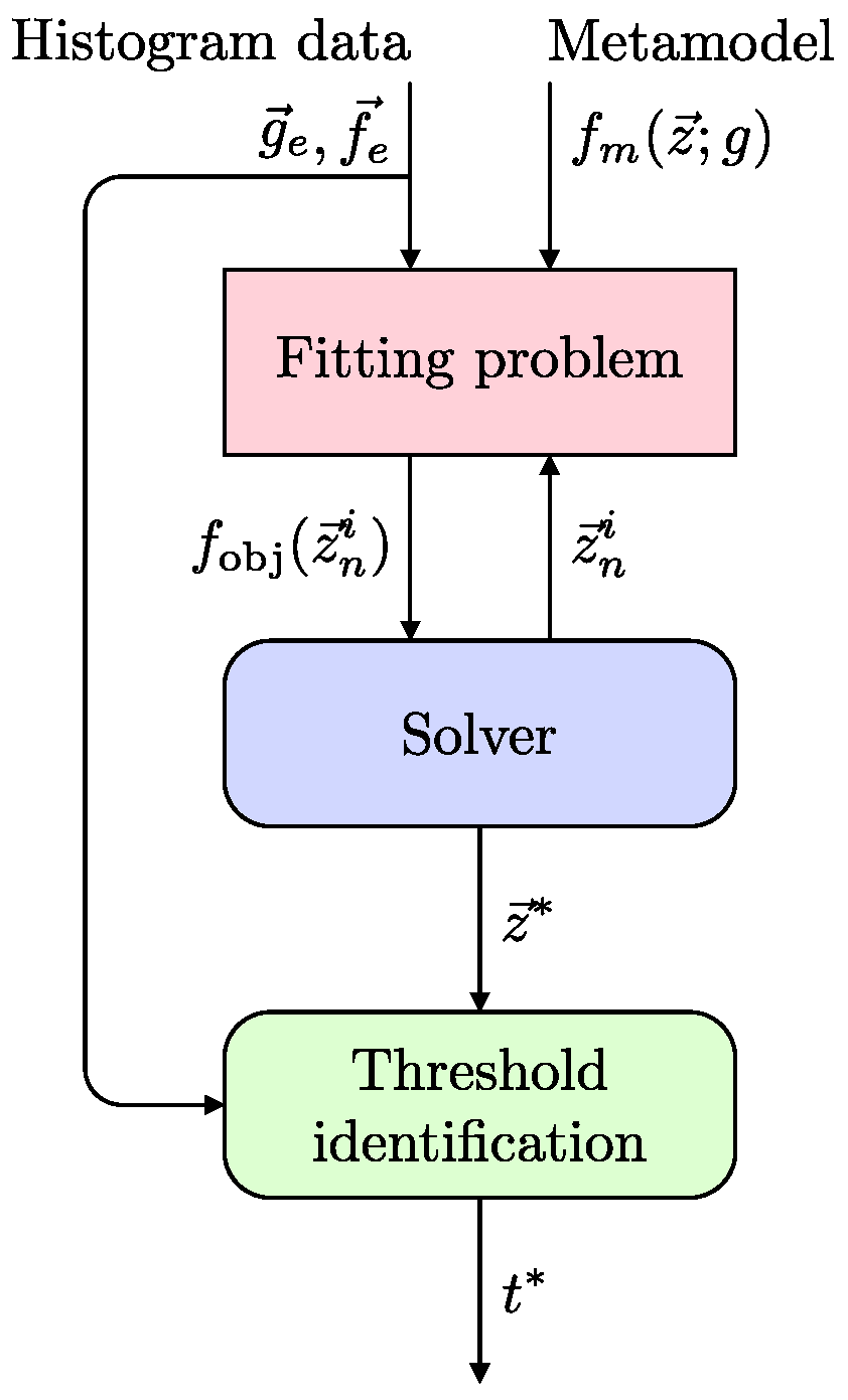
The proposed methodology employs two main procedures. The first one comprises the fitting problem of a metamodel $f_m(\overrightarrow{z};g)$ based on the Generalized Gaussian (GG) function and the histogram data (${\overrightarrow{g}}_e,{\overrightarrow{f}}_e$) from a gray image. This minimization problem is given by

$${\overrightarrow{z}}^{\ast }=\underset{\overrightarrow{z}\in {\mathfrak{Z}}^D}{argmin}{∥{\overrightarrow{f}}_e-{\overrightarrow{f}}_m(\overrightarrow{z};{\overrightarrow{g}}_e)∥}_2^2,$$

(17)

since $\overrightarrow{z}$ stands the metamodel parameters. A metaheuristic solver such as the Cuckoo Search Algorithm (CSA) is implemented to deal with such a problem. The second procedure then utilizes the information from the optimal parameters ${\overrightarrow{z}}^{\ast }$ and the histogram data to identify the threshold. Figure 1 illustrates the aforementioned proposed methodology. The remainder of this section details the metamodel, the optimization algorithm, and the threshold identification.

3.1. Generalized Gaussian Function

The sum of Generalized Gaussian Distributions (GGDs) is proposed as a metamodel according to [36]. The major feature of a GGD is its ability to approach several statistical distributions by only varying a parameter $\alpha$, such as the Impulsive ($\alpha \to 0$), sub-Laplacian ($\alpha <1$), Laplacian ($\alpha =1$), Gaussian ($\alpha =2$), and uniform ($\alpha \to \infty$) ones. Given this flexibility, we considered that GGDs are excellent candidates to describe the statistical characteristics presented in an image histogram as a meta-distribution.

We assumed that the histogram for the background and object shows two principal lobes (bimodal histogram); based on (13), it is proposed $f_m\left(g\right):{\mathbb{Z}}_G\mapsto [0,1]$ to approximate two probability density functions, such as

$$f_m(\overrightarrow{z};g)=f_1(\overrightarrow{z};g)+f_2(\overrightarrow{z};g).$$

(18)

In this distribution model, $f_k(\overrightarrow{z};g):{\mathbb{Z}}_G\mapsto [0,1]$ is given by

$$f_k\left(g\right)=G_{k}exp\left(-{\left|\frac{g-{\mu }_k}{{\sigma }_k}\right|}^{{\alpha }_k}\right),\forall k\in \{1,2\},$$

(19)

where $g\in {\mathbb{Z}}_G$, ${\mu }_k\in \mathbb{R}$, ${\sigma }_k\in {\mathbb{R}}_{+}$, and ${\alpha }_k\in {\mathbb{R}}_{+}$ are the intensity of the gray level, its mean, scale, and shape, respectively. Moreover, $\overrightarrow{z}$ is the parameter vector and $G_k\in {\mathbb{R}}_{+}$ is the normalizing constant defined by

$$G_k=\frac{{\alpha }_k}{2{\sigma }_k\mathsf{\Gamma }(1/{\alpha }_k)},\forall k\in \{1,2\}.$$

(20)

We consider $G_1$ and $G_2$ as two global constants to avoid the use of the $\mathsf{\Gamma }(·)$ function and thus to reduce the computational complexity; i.e., they are specified in parameter vector $\overrightarrow{z}={(G_1,{\mu }_1,{\sigma }_1,{\alpha }_1,G_2,{\mu }_2,{\sigma }_2,{\alpha }_2)}^{⊺}$. Furthermore, we set a simple constraint to this model to facilitate its analysis, such as ${\mu }_1<{\mu }_2$.

3.2. Cuckoo Search Algorithm

Cuckoo Search Algorithm (CSA) is a metaheuristic optimization method based on a population, and Lévy flights [37]. CSA mimics the brood parasitism behavior of certain cuckoo species, which hide their eggs inside alien nests. The general scientific community has widely accepted this method in numerous variants and applications [38,39,40]. CSA can be implemented to tackle a given minimization problem, such as

$${\overrightarrow{z}}^{\ast }=\underset{\overrightarrow{z}\in {\mathfrak{Z}}^D}{argmin}{f}_{\mathrm{obj}}\left(\overrightarrow{z}\right),$$

(21)

where ${\overrightarrow{z}}^{\ast }$ is the optimal solution and $f_{\mathrm{obj}}\left(\overrightarrow{z}\right)$ is the objective function. For maximization problems, such as those mentioned in Section 2.2, this objective function is just the negated threshold metric.

In CSA, the population is defined as $Z^t=\{{\overrightarrow{z}}_1\left(t\right),\cdots ,{\overrightarrow{z}}_N\left(t\right)\}\in \mathfrak{Z}$, since i is the time step, N is the number of agents, and D implies the dimensionality of the problem. Thus, ${\overrightarrow{z}}_n\left(t\right)\in Z\left(t\right)$ is the n-th agent’s position in the feasible domain $\mathfrak{Z}\subseteq {\mathbb{R}}^D$ at the step i. For most problems, such a domain $\mathfrak{Z}$ is defined as shown,

$$\mathfrak{Z}=\left\{\overrightarrow{z}\in {\mathbb{R}}^D:\left(\exists \overrightarrow{l},\overrightarrow{u}\in {\mathbb{R}}^D\right)\left[\overrightarrow{l}⪯\overrightarrow{z}⪯\overrightarrow{u}\right]\right\}$$

(22)

since $\overrightarrow{l}$ and $\overrightarrow{u}$ are the lower and upper boundary vectors, respectively.

As first step, the population is initialized at random within the problem domain, i.e., $Z^0\ni {\overrightarrow{z}}_n^0\ni z_{d,n}\sim \mathcal{U}(l_d,u_d)$$\forall l_d\in \overrightarrow{l},u_d\in \overrightarrow{u}$, and the fitness value for each agent is evaluated such that $f_n^0=f_{\mathrm{obj}}\left({\overrightarrow{z}}_n^0\right),\forall {\overrightarrow{z}}_n^0\in Z^0$. Then, the initial best position ${\overrightarrow{z}}^{0,\ast }$ and its fitness value $f^{0,\ast }$ are found, ${\overrightarrow{z}}^{0,\ast }=argmin\left\{f\left(Z^0\right)\right\}$, and the iteration counter is increased as $i\leftarrow i+1$. CSA employs the Lévy flight and local random walk as its primary two search mechanisms, which are applied iteratively until a convergence criterion, which was defined previously, is met. Some examples of the criteria are the maximum number of steps $i\ge i_{\max }$ and the best-fitness change tolerance $f^{i,\ast }-f^{i-1,\ast }\le \epsilon$.

Thence, the Lévy flight for the n-th agent (${\overrightarrow{z}}_n^i\in Z^i$) is given by

$${\overrightarrow{z}}_n^i={\overrightarrow{z}}_n^i+\zeta \overrightarrow{\eta }\odot ({\overrightarrow{z}}_n^{i-1}-{\overrightarrow{z}}^{i-1,\ast }),$$

(23)

where $\zeta >0$ is the spatial step size, $\overrightarrow{\eta }$ is a vector of i.i.d. random numbers obtained from the Mantegna–Stanley’s algorithm [41] using the symmetric Lévy stable distribution, and ⊙ is the Hadamard–Schur’s product.

Likewise, the second procedure, namely, local random walk, is defined as

$${\overrightarrow{z}}_n^i={\overrightarrow{z}}_n^i+\overrightarrow{r}\odot H(\overrightarrow{r}-p)\odot ({\overrightarrow{z}}_{q_1}^i-{\overrightarrow{z}}_{q_2}^i),$$

(24)

where $\overrightarrow{r}$ is a vector of i.i.d. random variables with $\mathcal{U}(0,1)$, $p\in [0,1]$ is the probability of change, and $H:{\mathbb{R}}^D\to {\mathbb{Z}}_2^D$ is the element-wise Heaviside step function with $H\left(0\right)=1$. Indices $q_1$ and $q_2$ are mutually exclusive integers randomly selected from the population range $[1,N]$.

After applying each of these search mechanisms, all agents are evaluated in the objective function, and only the new positions ${\overrightarrow{z}}_n^i$ better than the previous ones ${\overrightarrow{z}}_n^{i-1}$ are preserved, i.e., ${\overrightarrow{z}}_n^i={\overrightarrow{z}}_n^{i-1}$ if $f_n^i>f_n^{i-1},\forall n\in \{1,\cdots ,N\}$. Furthermore, once the local random walk is performed and the population is updated, the best position ${\overrightarrow{z}}^{i,\ast }$ and its fitness value $f^{i,\ast }$ are found as they were before with the initial population. Thus, the convergence criteria are checked. If any are satisfied, the iterative procedure concludes. Otherwise, the step counter is increased $i=i+1$, and the search mechanisms are applied again.

3.3. Threshold Identification

The threshold identification procedure is somewhat similar to those described in Section 2. The main differences are that instead of using the histogram data ($g_e,f_e$), we evaluate a subset of gray-scale levels $T\subset G$ over the fitted GGD model $f_m({\overrightarrow{z}}^{\ast };t)$. We stress that we do not employ the direct histogram data but the fitted curves. Thus, his subset T is obtained as follows

$$T=\left\{g\in {\overrightarrow{g}}_e:\left(⌊{\mu }_1^{\ast }+{\sigma }_1^{\ast }/2⌋<g<⌈{\mu }_2^{\ast }-{\sigma }_2^{\ast }/2⌉\right)\left[⌊{\mu }_1^{\ast }+{\sigma }_1^{\ast }/2⌋<⌈{\mu }_2^{\ast }-{\sigma }_2^{\ast }/2⌉\right]\right\},$$

(25)

where ${\mu }_1^{\ast }$, ${\sigma }_1^{\ast }$, ${\mu }_2^{\ast }$, and ${\sigma }_2^{\ast }$ are from the optimal parameter values ${\overrightarrow{z}}^{\ast }$ achieved in the optimization procedure. The rounding operators $\lfloor ·\rfloor$ and $\lceil ·\rceil$ stand the floor and ceil, respectively. This subset will be nonempty, at least in the context of the segmentation problem tackled in this work. Hence, the optimal threshold value using the proposed method is found as shown

$$t^{\ast }=\underset{t\in T}{argmin}\left\{f_m({\overrightarrow{z}}^{\ast };t)\right\}.$$

(26)

4. Methodology

We carried out a three-fold experiment procedure to study the proposed method ThCSA and also to compare it against those methods described in Section 2.2. These methods are Otsu, Matlab’s Otsu implementation (GrayThresh), Maximum Entropy (MxE), Kittler–Illingworth (KI), and ThCSA. The graythresh method is omitted for simulated comparison because it requires an image as input. We tested the methods using simulated distributions in the preliminary experiment, which correspond to bimodal histograms with the optimal threshold $t_{r1}^{\ast }$ as a reference. The optimal threshold is obtained with the intersection of two well-known distributions. In this work, the sum of distributions was designated as a global histogram. For this experiment, the synthetic histogram was considered as the sum of two distributions, not a histogram in the strict sense. Synthetic histograms have constant parameters to simulate two distributions.

Table 1. Simulated histograms utilized as study cases for the preliminary experiment. Parameters ${\alpha }_k$, ${\sigma }_k$, and ${\mu }_k$, $\forall k=\{1,2\}$, correspond to the distribution model in (19).

Simulation	${\mathit{\alpha }}_1$	${\mathit{\alpha }}_2$	${\mathit{\sigma }}_1$	${\mathit{\sigma }}_2$	${\mathit{\mu }}_1$	${\mathit{\mu }}_2$
$s_{01}$	1	1.62	30.61	43.60	58	183
$s_{02}$	2	1.42	40.62	33.06	78	163
$s_{03}$	2	1.71	46.17	48.12	56	187
$s_{04}$	1	1.38	42.05	38.85	64	195
$s_{05}$	2	0.97	32.58	33.81	68	175

describes the five cases that comprise this experiment. In the first experiment, we simulated a bimodal histogram corresponding to an image with one object and a well-defined background with two known thresholds.

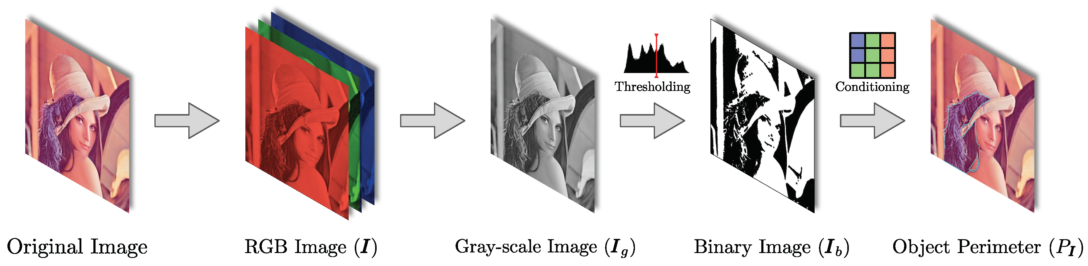
The remainder experiments were performed following the procedure depicted in Figure 2. First, the original image is read as an RGB image $\mathit{I}\in {\mathbb{Z}}_G^{M\times N\times 3}$ and then transformed to gray-scale ${\mathit{I}}_g\in {\mathbb{Z}}_G^{M\times N}$. The gray-scale image serves to obtain the histogram $f\left(g\right)$, as commented in Section 2, except for the GrayThresh method, which utilizes the image ${\mathit{I}}_g$ directly. Therefore, the thresholding methods are applied to achieve the binary image ${\mathit{I}}_{b_1}\in {\mathbb{Z}}_2^{M\times N}$. Lastly, the object perimeter $P_{\mathit{I}}$ is detected by locating the isolines of the processed ${\mathit{I}}_{b_1}$ image. The general methodology is summarized in Pseudocode 1.

The second set of experiments consisted of segmenting samples of melanoma images collected from the PH2 Dermoscopic Image Database [42]. We selected this particular image database mainly because the reference images of the melanoma area are provided and supported by expert dermatologists. In addition, these images present histograms with diversity in their statistical parameters and the distances and amplitudes of the histogram’s main lobes. It is worth mentioning that these samples required a special consideration to compute the perimeter of skin lesion; this fact is detailed in the next section. The final experiments comprised the segmentation of organic and inorganic products with a non-uniform background. To do this, we implemented the procedure mentioned above with three images acquired for this work.

Pseudocode 1 Proposed procedure for image segmentation and contour computing
Input: Original image $\mathit{I}$ and thresholding method ThresholdingMethod Output: Processed binary image ${\mathit{I}}_{b_1}$ and perimeter $P_{\mathit{I}}$
1:${\mathit{I}}_g\leftarrow GrayScale\left(\mathit{I}\right)$	▹ Transform from RGB to gray-scale
2:$t\leftarrow ThresholdingMethod\left({\mathit{I}}_g\right)$	▹ Threshold t computed with a given method
3:${\mathit{I}}_{b_1}\leftarrow Binarize({\mathit{I}}_g,t)$	▹ Binarization according to t
4:$P_{\mathit{I}}\leftarrow Contour\left({\mathit{I}}_{b_1}\right)$	▹ Draws a contour of ${\mathit{I}}_{b_1}$

The methodology described in Figure 2 was designed to apply a traditional thresholding procedure and the basic image form (a binary image) to identify the object perimeter. The object perimeter for the second and third experiments is determined for different reasons. The melanoma perimeter helps to provide a view of the morphological structure of skin lesions, which can be used to support a clinic diagnosis [42]. Meanwhile, the methodology proposed for the second experiment can be employed to distinguish between organic and inorganic objects. This is due to the number of centroids of the identified object perimeters.

Moreover, all the experiments were run on a machine with an Intel Core i5 @ 1.6 GHz CPU, 4.00 GB @ 1600 MHz RAM, using the numerical platforms Matlab R2018a and R v4.0.3. We implemented Cuckoo Search Algorithm (CSA) with a population size N of 200, a step size $\zeta$ of 1.0, a probability change p of 0.5, a best-fitness change tolerance $\epsilon$ of ${10}^{-15}$, and a maximum number of stagnating iterations of 2000. These values were obtained after performing a preliminary study, which is out of this work’s scope but can be consulted in [43].

5. Results and Discussion

The first experiment consists of implementing the proposed method and the others from the literature (ThCSA, Otsu, MxE, and KI) on synthetic histograms (cf. Section 4).

Table 2. Comparison of threshold values obtained by different methods in a simulated environment. Based on the optimal threshold $t_{r1}^{\ast }$, the symbols ↓ and ↑ indicate the worst and the best threshold respectively.

Simulation	${\mathit{t}}_{\mathit{r}1}^{\ast }$	Otsu	MxE	KI	ThCSA
$s_{01}$	120	121 ${}^{\uparrow }$	128 ${}^{\downarrow }$	113	116
$s_{02}$	122	120 ${}^{\uparrow }$	119 ${}^{\downarrow }$	120 ${}^{\uparrow }$	120 ${}^{\uparrow }$
$s_{03}$	119	122${}^{\downarrow }$	118${}^{\uparrow }$	121	121
$s_{04}$	135	129	140 ${}^{\uparrow }$	127${}^{\downarrow }$	129
$s_{05}$	114	125 ${}^{\downarrow }$	119	119	118${}^{\uparrow }$

presents the resulting thresholds from this simulation comparison, where the symbols ↓ and ↑ indicate the worst and the best thresholds, respectively. This is based on the optimal threshold. In the first simulation $s_{01}$, Otsu yields the closest values to the optimal threshold. Meanwhile, ThCSA achieved a threshold value with a difference of four gray intensity values from the optimal reference. Finally, the worst result was attained by MxE. From the results achieved in simulation $s_{02}$, it is easy to notice that Otsu, KI and ThCSA had the same performance, closely followed by MxE. In $s_{02}$, it is worth noticing that Otsu, KI and ThCSA computed a threshold near to the optimal threshold with a difference of two gray intensity levels, respectively. Moreover, the thresholds attained for the simulation $s_{03}$ are diverse. For this simulation, MxE outperforms the other methods according to the optimal reference. It is noticeable that Kittler and ThCSA share the the same threshold, with a difference of two gray intensity values from $t_{r1}^{\ast }$. The worst algorithm to assess the reference threshold was found to be Otsu, with a minimal difference of three gray levels. Now, based on the results shown in Table 2 for simulation $s_{04}$, we observe that MxE exhibits an advantage over other algorithms for the optimal threshold. Here, Otsu and ThCSA obtained the same level and reached second place with a difference of six gray intensity levels. The last simulation, $s_{05}$, yields interesting results. In this scenario, ThCSA render the best threshold concerning the optimal threshold. Meanwhile, MxE and Kittler rank at an intermediate level according to the reference threshold. In this simulation, the algorithm Otsu obtained the lowest performance.

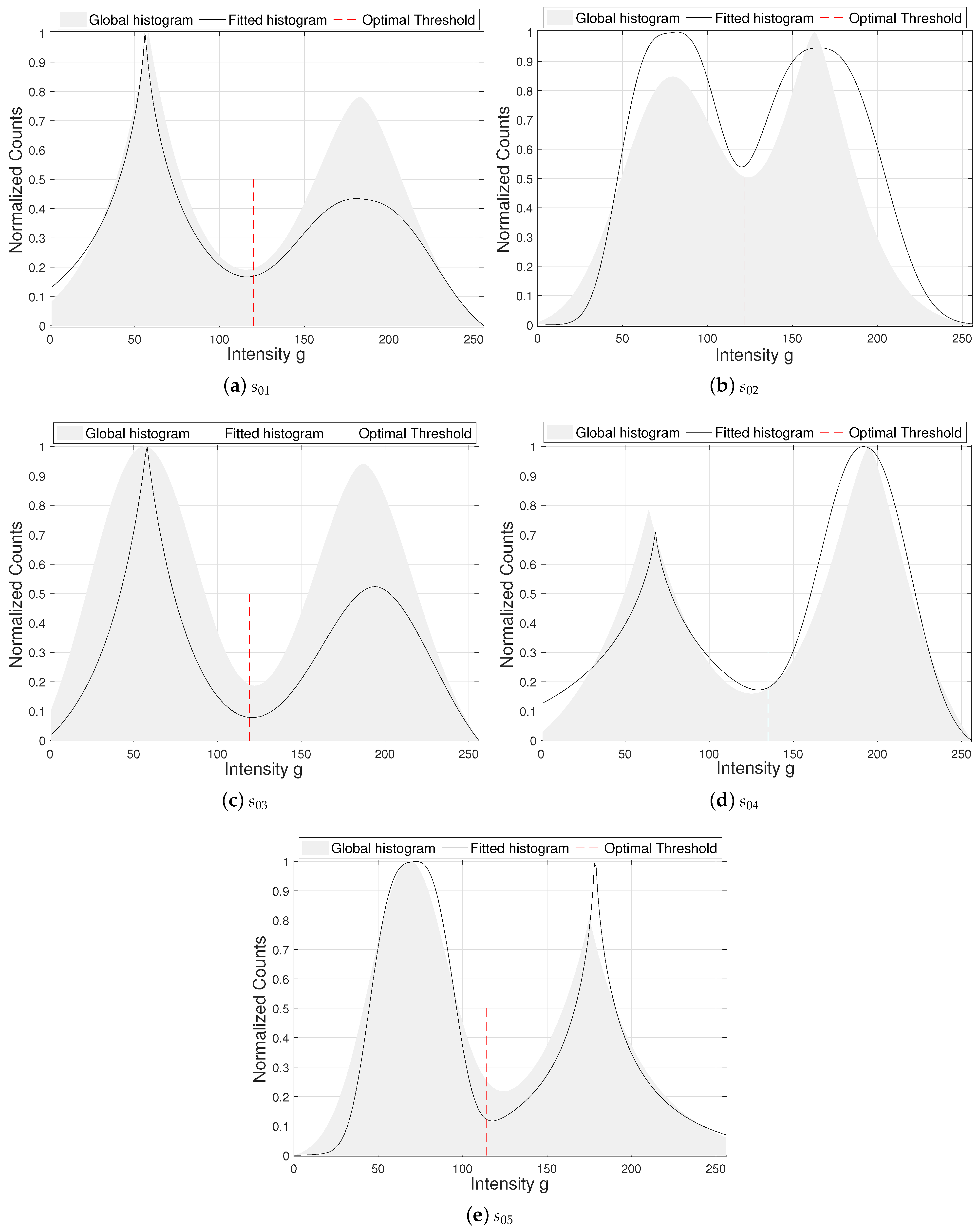
Figure 3 illustrates the cases of those simulated distributions, the optimal threshold and estimated histograms obtained by using ThCSA. In these plots, the fitted histograms (in black solid lines) evidence an outstanding description of the global histogram, especially regarding the reference threshold (in red dashed line). Nevertheless, we observe two issues in these resulting histograms: In the first one in Figure 3a, the right-hand side distribution is lower than the simulated data. Plus, in the second one in Figure 3b, an unsatisfactory fitting of the right and left hand side peaks is evident. In Figure 3c the right-hand and left-hand side distributions are narrower and lower than simulated histogram, respectively.

Subsequently,

Table 3. Thresholds detected in medical Images with different methods and variables identified by Cuckoo Search Algorithm.

Image	Thresholds of Medical Images					Optimal Variables Identified via CSA
	Otsu	GrayThresh	KI	MxE	ThCSA	${\mathit{G}}_1^{\ast }$	${\mathit{G}}_2^{\ast }$	${\mathit{\mu }}_1^{\ast }$	${\mathit{\mu }}_2^{\ast }$	${\mathit{\sigma }}_1^{\ast }$	${\mathit{\sigma }}_2^{\ast }$	${\mathit{\alpha }}_1^{\ast }$	${\mathit{\alpha }}_2^{\ast }$
IMD002	136	127	132	146	138	0.23	0.92	96	180	31.46	26.71	3.0	3.0
IMD004	162	127	177	169	139	0.10	1.05	91	229	35.73	17.84	1.6	0.6
IMD015	143	127	143	159	125	0.69	0.98	93	192	10.34	25.69	1.4	1.5
IMD021	120	119	123	133	112	0.1	0.84	74	158	24.29	11.85	1.6	1.0
IMD041	157	156	158	169	156	0.36	0.9	97	215	30.71	31.51	1.1	2.3

shows the thresholds comparison obtained with the algorithms implemented for segmenting four dermoscopic images, i.e., IMD002, IMD004, IMD015, IMD021, and IMD041. As we mentioned in Section 4, we chose these figures to illustrate histograms with different patterns. The optimal variables achieved by CSA for the GG distributions are also presented. Recall that the ${\alpha }_1$ and ${\alpha }_2$ values describe abnormal distributions when ${\alpha }_k\ne 2\forall k\in \{1,2\}$. It is worth noting that the thresholds estimated by ThCSA and Otsu for the IMD002 sample are close. Hence, the histogram of IMD002 is enveloped with a sum of non-Gaussian distribution because ${\alpha }_1^{\ast }=3$ and ${\alpha }_2^{\ast }=3$. In the second test, using IMD004, ThCSA estimates a classification edge with an average variation of ca. 29 intensities w.r.t. the other algorithms. The distributions computed have the shape parameters ${\alpha }_1^{\ast }=1.6$ and ${\alpha }_2^{\ast }=0.6$, which correspond to sub-Gaussian and sub-Laplacian distributions, respectively. For IMD015 and IMD021, ThCSA and GrayThresh achieve similar thresholds. It can also be observed in Table 3 that the shape parameters to this sample are located at $1\le {\alpha }_1^{\ast },{\alpha }_2^{\ast }<2$, i.e., between Laplacian and Gaussian distributions. For this experiment, the estimated characteristics can be described with the following ranges $0.1\le G_1^{\ast },G_2^{\ast }\le 0.98$, $74\le {\mu }_1^{\ast },{\mu }_2^{\ast }\le 192$, $10.34<{\sigma }_1^{\ast },{\sigma }_2^{\ast }<25.69$, and $1<{\alpha }_1^{\ast },{\alpha }_2^{\ast }<2$. Finally, the proposed algorithm and GrayThresh obtained the same threshold for IMD041. These results can corroborate the flexibility of the proposed algorithm to estimate several parameters at the same time on a different scale.

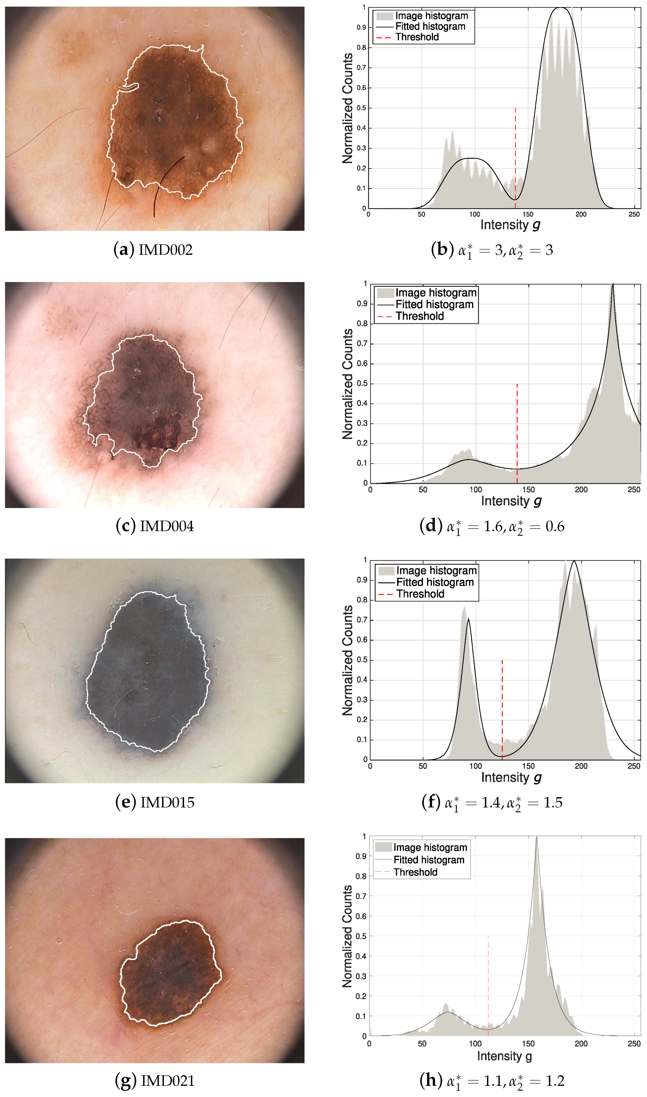
Complementing the information achieved in this experiment, as described in Figure 2, we determine the contours $P_{\mathit{I}}$ for the medical images IMD002, IMD004, IMD015, and IMD021. The segmentation of medical samples generates extra white corners following the procedure depicted in Figure 2 and Pseudocode 1. For this particular case, it is required to remove the contour located in the corner of each image. Figure 4a,c,e,g show the resulting contours $P_{\mathit{I}}$ in RGB images, which is computed with the isolines of processed ${\mathit{I}}_{b_1}$ image and depicted with a solid line. Therefore, the contour $P_{\mathit{I}}$ helps to determine the dark area of melanoma samples.

Figure 4b,d,f,h illustrate the image histogram (gray patch), fitted histogram (black solid line), and estimated threshold (red dashed line) with ThCSA. In these images, one can observe two principal lobes and a valley between them, where the threshold achieved with ThCSA is located. It is also possible to appreciate the estimated distributions with several shape parameters, which are denoted with ${\alpha }_1^{\ast }$ and ${\alpha }_2^{\ast }$ to the first and second lobes, respectively. Additionally, we can notice some discrepancies between the estimated distributions and the histograms in Figure 4b,d,f,h. However, the parameters estimated using ThCSA are able to determine a threshold that achieves the segmentation of the melanoma area.

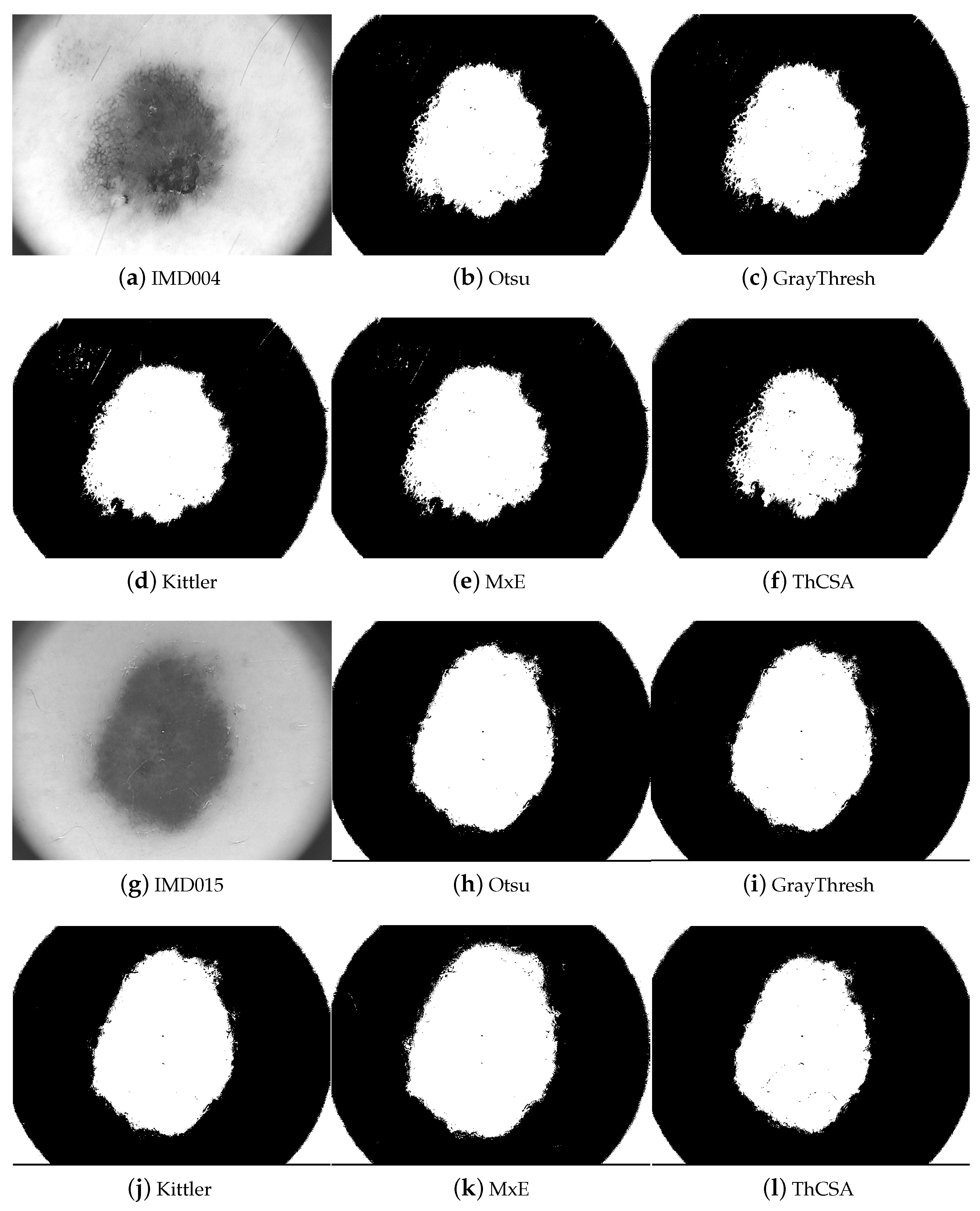
To complement the previous results, we focus on the visual and numeric comparison of the segmentation outcomes for the medical samples. The segmentation results of IMD004 and IMD015 using the studied algorithms in the are shown in Figure 5. Here, the Otsu methods in Figure 5b, GrayThresh in Figure 5c, Kittler in Figure 5d, MxE in Figure 5e, and ThCSA in Figure 5f obtained similar results for the sample IMD004 in Figure 5a. These images display white corners in the background, i.e., additional white pixels as a component of the skin lesion, which could be removed with additional processing. Some additional white pixels in the segmented background can also be observed using the Kittler, Figure 5d, and MxE, Figure 5e, methods. Based on the same algorithms, the sample IMD015, shown in Figure 5g, is segmented. By using this sample, the algorithms obtained an equivalent segmentation. This can be corroborated for Otsu, GrayThresh, Kittler, MxE, and ThCSA in Figure 5h–l, respectively. Here, the segmented skin lesion is more uniform, without extra white pixels in the background, independent of the corner area. For this sample, all segmentations illustrated in Figure 5h–l, recognize a line of black pixels in the bottom as background components. This error is caused by extra white pixels immersed in the original RGB image.

Naturally, the visual comparison is insufficient to determine the best algorithm. For this reason, the reference images of melanomas or ground-truth images are required. Such images are provided by an expert dermatologist in [42], which are represented as ${\mathit{I}}_{b_r}\in {\mathbb{Z}}_2^{M\times N}$. ${\mathit{I}}_{b_r}\in {\mathbb{Z}}_2^{M\times N}$.

Table 4. Jaccard index and False Negative (FN) values obtained via different methods for medical samples. The best Jaccard index is in bold font. Symbols ↑ and ↓ represent the worst and best values, respectively.

Method	IMD002		IMD004		IMD015		IMD021		IMD041
	Jaccard	FN	Jaccard	FN	Jaccard	FN	Jaccard	FN	Jaccard	FN
Otsu	0.6889	0.1296	0.6645	0.0421	0.7117	0.0070	0.6149	0.0206	0.6818	0.0746
GrayThresh	0.6868	0.1362	0.6664	0.0447	0.7157	0.0080	0.6176	0.0242	0.6822	0.0779 ↑
Kittler	0.6780	0.1577↑	0.6167	0.0143↓	0.7117	0.0070	0.6062	0.0140	0.6816	0.0707
MxE	0.6939	0.0786↓	0.6471	0.0263	0.6244	0.0007↓	0.5555	0.0036↓	0.6669	0.0362 ↓
ThCSA	0.6917	0.1189	0.6601	0.1428↑	0.7551	0.0496 ↑	0.6256	0.0558↑	0.6822	0.0779↑

shows the Jaccard index and the False Negative (FN) pixels for all the methods. The Jaccard index is used to evaluate the image segmentation because it measures the intersection of an obtained binary image (${\mathit{I}}_{b_1}$ or ${\mathit{I}}_{b_2}$) and the reference image (${\mathit{I}}_{b_r}$) divided by the union of both images [44]. The FN points are the unmatched pixels of the segmented image and the area labeled as object ${\mathit{I}}_{O_r}$ in the reference image, where ${\mathit{I}}_{O_r}\subset {\mathit{I}}_{B_r}$. Employing the FN metric, it is possible to identify which method locates fewer wrong pixels in the object. In Table 4, the FN values are divided by the total number of pixels of ${\mathit{I}}_{O_r}$ to avoid large numbers. These metrics are obtained for different melanoma images IMD002, IMD004, IMD015, IMD021, and IMD041. Table 4 displays the best Jaccard index in bold font. According to the Jaccard index, we can appreciate that, for IMD002, the best algorithm is MxE. This generates fewer inaccuracies regarding the FN values. Additionally, ThCSA ranks second according to the Jaccard index. For IMD004, the GrayThresh method is the best one. The ThCSA showed the maximal number in the FN column, but this method is in third place. Moreover, we notice that ThCSA is better for the sample IMD015 according to the Jaccard index, although the proposed algorithm obtained the worst values in FN measurements. For the sample IMD021, ThCSA was better than the other algorithms. However, the proposed algorithm obtained a low performance for FN values. The last sample analyzed was the image IMD041. Here, the algorithms GrayThresh and ThCSA were the best options, with the same Jaccard index and FN measures.

It is worth noting that the Jaccard indices are quite low, in the range of 0.6–0.8. This poor performance is due to the extra white pixels located in the corners of the images. However, the Jaccard index is adequate to rank the proposed algorithm. Furthermore,

Table 5. Computing time required to find the threshold for medical images with different methods.

Method	Computing Time [s]
	IMD002	IMD004	IMD015	IMD021	IMD041
Otsu	0.03	0.04	0.02	0.03	0.4
GrayThresh	0.02	0.02	0.02	0.03	0.2
Kittler	0.01	0.02	0.01	0.02	0.2
MxE	0.04	0.04	0.03	0.04	0.04
ThCSA	1.5	1.2	1.3	1.4	1.1

shows the computing time comparison between the implemented algorithms. From these data, we can recognize the high computing time as a drawback of the proposed algorithm. Nevertheless, we suggest that this comparison is unfair because all the algorithms studied in this work were employed on different numerical platforms.

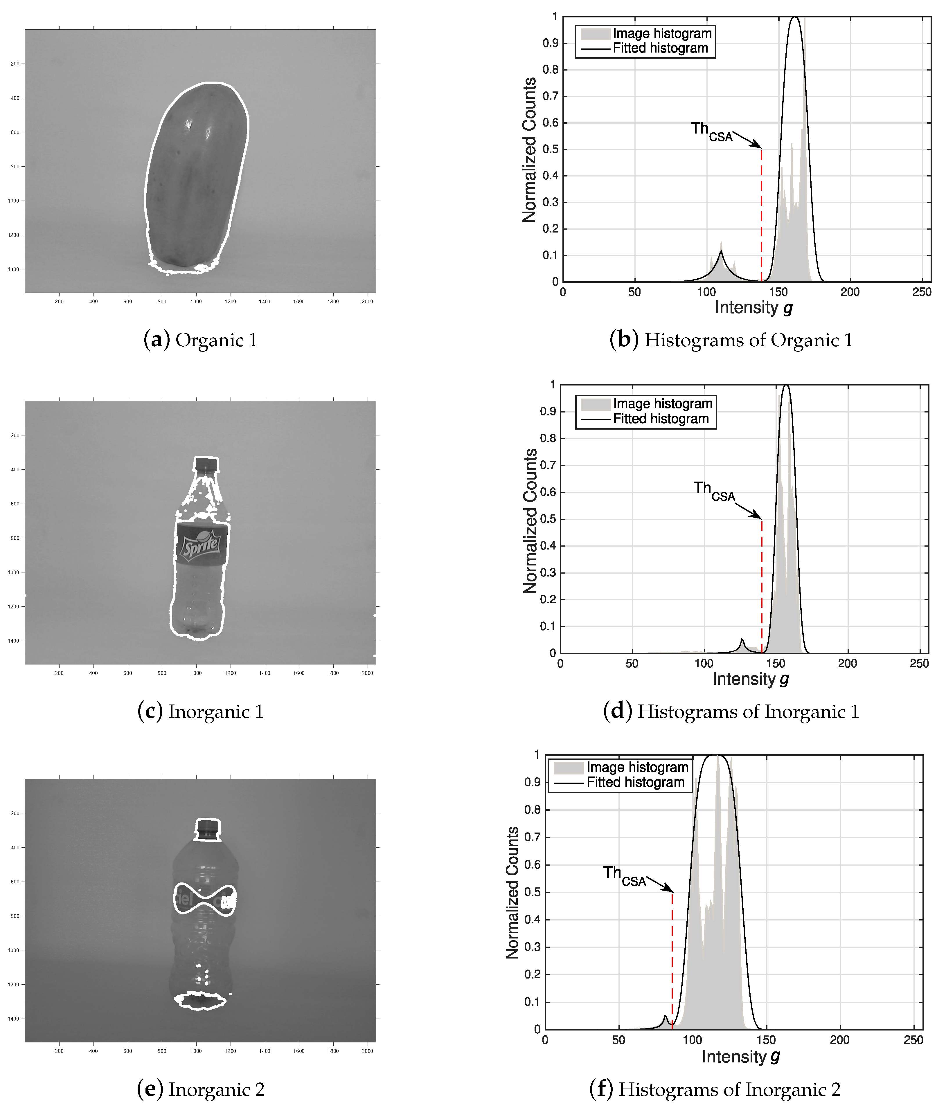
Furthermore, we extend the scope of application of the proposed algorithm by studying other kinds of images. To do this, we considered those with a background covering a greater area than the object. Sometimes the objects share pixels with the background in the gray-scale image. Figure 6 depicts three examples of this problem: one organic product and two inorganic products. The organic one is illustrated in Figure 6a, and its histogram is plotted in Figure 6b. The image in gray-scale, see Figure 6a, illustrates a background with different shades of gray and a darker area, representing the organic object. The histogram in Figure 6b shows two no uniform lobes that corroborate the color variability of the object and background. These lobes are approximately $G=90$ to $G=130$ for the object, and from $G=140$ to $G=175$ for the foreground. Despite fluctuations in the histogram, depicted in Figure 6b, the algorithm ThCSA computed a good threshold to segment the organic object, which is bounded with a white line in Figure 6a.

Moreover, the two inorganic, which possess transparent areas, are shown in Figure 6c,e, and their histograms in Figure 6d,f, respectively. In Figure 6c, a white line delineates partially incomplete area of an inorganic product. This is because some object pixels are mixed with the background; i.e., they have the same intensity level. Figure 6d shows the threshold achieved by the ThCSA-based methodology. This threshold helps to delimit a large part of the object, although the object’s outline is incomplete. Finally, in Figure 6e,f, we observe the most challenging example of this proposed work. To this inorganic object, the bottom, the label, and the screw cap are identified. The histograms (see Figure 6f) evidence where there is little information about the object. However, the proposed methodology can compute the corresponding thresholds to identify parts of this object.

6. Conclusions

In this work, we proposed ThCSA, a thresholding technique based on the Generalized Gaussian (GG) distributions and Cuckoo Search Algorithm. We implemented this methodology to tackle several image segmentation cases with different conditions and compared its results with some well-known algorithms. We showed that ThCSA, Otsu, and MxE obtain acceptable results when estimating the optimal threshold in simulated histograms. However, Otsu and MxE achieved the worst mark in at least one simulation, and GrayThresh was the worst at estimating the reference threshold. According to the comparison, the proposed algorithm obtained good performances by computing thresholds with a minimal difference and values very close to the optimal reference in most cases. These results are closely followed by the Kittler–Illingworth (KI).

ThCSA achieved the GG function variables in real medical image-processing to determine a threshold that segments the melanoma samples. The skin lesions were bounded with a certain precision based on the proposed methodology. Compared with the manual segmentation (ground-truth), evaluated by an expert dermatologist, the best segmentations were rendered by ThCSA, closely followed by GrayThresh. We corroborated this affirmation through the Jaccard indices, which can be improved with additional processing to avoid the corners induced by the capture instrument.

Furthermore, we noticed a remarkable potential when applying ThCSA to identify objects with no-uniform backgrounds and shared pixels. However, we found some issues while delimiting the complete object by the proposed method, especially when the background and object pixels have the same gray levels. Notwithstanding, ThCSA can detect strategic points to locate parts of the object. This issue should be analyzed and solved with an additional processing step. The principal disadvantage of the proposed methodology is that it requires more processing time than the other methods. Nevertheless, naturally, this work addressed the prototyping of an algorithm that could be enhanced and optimized in future implementations. Therefore, considering the advantages and disadvantages mentioned above, we finally conclude that the proposed methodology is an excellent option to compute optimal thresholds and segment objects from its quasi-uniform environment. This work presented an alternative thresholding tool, based on a global optimization algorithm, to help practitioners in diverse applications, e.g., dermatologic ones. Moreover, we plan to compare ThCSA with different image databases and employ several metrics to measure the segmentation quality for future work. We will also optimize the ThCSA implementation in a particular numerical platform to provide a competitive alternative to thresholding in any practical application.