
Arbitrary Coefficient Assignment by Static Output Feedback for Linear Differential Equations with Non-Commensurate Lumped and Distributed Delays


Abstract
:1. Introduction
2. Main Results
3. Corollaries
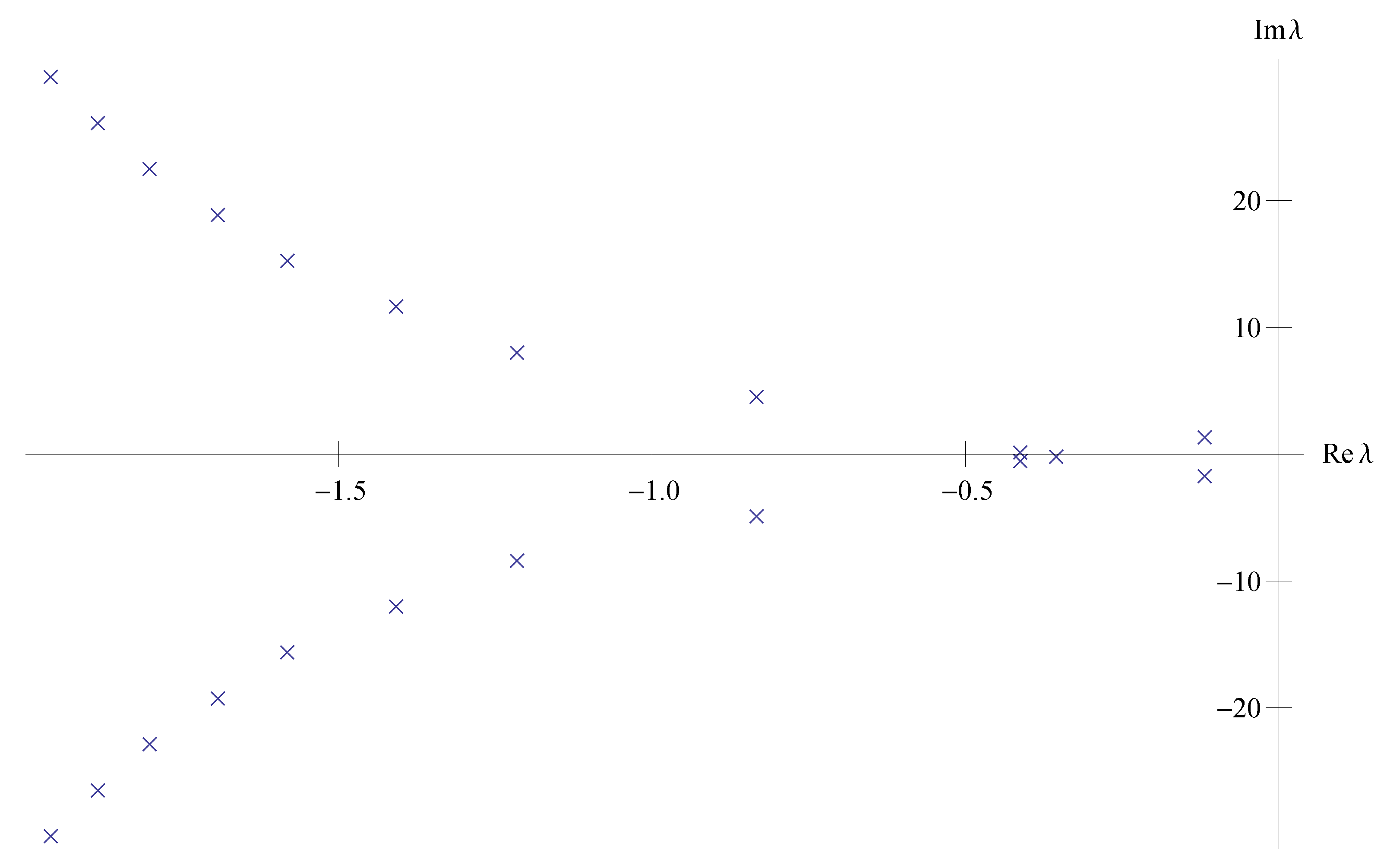
4. Modeling Example
5. Conclusions
Author Contributions
Funding
Acknowledgments
Conflicts of Interest
References
- Gu, K.; Niculescu, S.I. Survey on recent results in the stability and control of time-delay systems. J. Dyn. Syst. Meas. Control 2003, 125, 158–165. [Google Scholar] [CrossRef]
- Richard, J.-P. Time-delay systems: An overview of some recent advances and open problems. Automatica 2003, 39, 1667–1694. [Google Scholar] [CrossRef]
- Sipahi, R.; Niculescu, S.; Abdallah, C.T.; Michiels, W.; Gu, K. Stability and stabilization of systems with time delay. IEEE Control Syst. 2011, 31, 38–65. [Google Scholar] [CrossRef]
- Pekař, L.; Gao, Q. Spectrum analysis of LTI continuous-time systems with constant delays: A literature overview of some recent results. IEEE Access 2018, 6, 35457–35491. [Google Scholar] [CrossRef]
- Krasovskii, N.-N. Stability of Motion: Applications of Lyapunov’s Second Method to Differential Systems and Equations With Delay; Stanford Univerity Press: Stanford, CA, USA, 1964. [Google Scholar]
- Kharitonov, V.L.; Zhabko, A.P. Lyapunov–Krasovskii approach to the robust stability analysis of time-delay systems. Automatica 2003, 39, 15–20. [Google Scholar] [CrossRef]
- Kharitonov, V.L. Time-Delay Systems; Birkäuser: Boston, MA, USA, 2013. [Google Scholar] [CrossRef]
- Egorov, A.V.; Cuvas, C.; Mondié, S. Necessary and sufficient stability conditions for linear systems with pointwise and distributed delays. Automatica 2017, 80, 218–224. [Google Scholar] [CrossRef]
- Michiels, W.; Niculescu, S.I. Stability and Stabilization of Time-Delay Systems. An Eigenvalue-Based Approach; SIAM: Philadelphia, PA, USA, 2007. [Google Scholar] [CrossRef]
- Popov, V.M. Hyperstability and optimality of automatic systems with several control functions. Rev. Roumaine Sci. Tech. Ser. Electrotech. Energy 1964, 9, 629–690. [Google Scholar]
- Wonham, W.M. On pole assignment in multi-input controllable linear systems. IEEE Trans. Automat. Control 1967, 12, 660–665. [Google Scholar] [CrossRef] [Green Version]
- Asmykovich, I.K.; Marchenko, V.M. Modal control of multiinput linear delayed systems. Autom. Remote Control 1980, 41, 1–5. [Google Scholar]
- Kono, M. Decoupling and arbitrary coefficient assignment in time-delay systems. Syst. Control Lett. 1983, 3, 349–354. [Google Scholar] [CrossRef]
- Lee, E.; Lu, W. Coefficient assignability for linear systems with delays. IEEE Trans. Automat. Control 1984, 29, 1048–1052. [Google Scholar] [CrossRef]
- Olbrot, A. Stabilizability, detectability, and spectrum assignment for linear autonomous systems with general time delays. IEEE Trans. Automat. Control 1978, 23, 887–890. [Google Scholar] [CrossRef]
- Kamen, E. Linear systems with commensurate time delays: Stability and stabilization independent of delay. IEEE Trans. Automat. Control 1982, 27, 367–375. [Google Scholar] [CrossRef]
- Lee, E.; Zak, S. On spectrum placement for linear time invariant delay systems. IEEE Trans. Automat. Control 1982, 27, 446–449. [Google Scholar] [CrossRef]
- Manitius, A.; Olbrot, A. Finite spectrum assignment problem for systems with delays. IEEE Trans. Automat. Control 1979, 24, 541–552. [Google Scholar] [CrossRef]
- Watanabe, K.; Ito, M.; Kaneko, M.; Ouchi, T. Finite spectrum assignment problem for systems with delay in state variables. IEEE Trans. Automat. Control 1983, 28, 506–508. [Google Scholar] [CrossRef]
- Watanabe, K.; Ito, M.; Kaneko, M. Finite spectrum assignment problem for systems with multiple commensurate delays in state variables. Int. J. Control 1983, 38, 913–926. [Google Scholar] [CrossRef]
- Watanabe, K.; Ito, M.; Kaneko, M. Finite spectrum assignment problem of systems with multiple commensurate delays in states and control. Int. J. Control 1984, 39, 1073–1082. [Google Scholar] [CrossRef]
- Watanabe, K. Finite spectrum assignment and observer for multivariable systems with commensurate delays. IEEE Trans. Automat. Control 1986, 31, 543–550. [Google Scholar] [CrossRef]
- Metel’skii, A.V. Finite spectrum assignment problem for a delay type system. Differ. Equ. 2014, 50, 689–699. [Google Scholar] [CrossRef]
- Metel’skii, A.V. Finite spectrum assignment problem for a differential system of neutral type. Differ. Equ. 2015, 51, 69–82. [Google Scholar] [CrossRef]
- Metel’skii, A.V. Modal controllability of a delay differential system by an incomplete output. Differ. Equ. 2018, 54, 1483–1493. [Google Scholar] [CrossRef]
- Zhou, B.; Liu, Q.; Mazenc, F. Stabilization of linear systems with both input and state delays by observer–predictors. Automatica 2017, 83, 368–377. [Google Scholar] [CrossRef] [Green Version]
- Belotti, R.; Richiedei, D. Pole assignment in vibrating systems with time delay: An approach embedding an a priori stability condition based on Linear Matrix Inequality. Mech. Syst. Signal Process. 2020, 137, 106396. [Google Scholar] [CrossRef]
- Dantas, N.J.B.; Dorea, C.E.T.; Araujo, J.M. Partial pole assignment using rank-one control and receptance in second-order systems with time delay. Meccanica 2021, 56, 287–302. [Google Scholar] [CrossRef]
- Zhu, Q. Stabilization of stochastic nonlinear delay systems with exogenous disturbances and the event-triggered feedback control. IEEE Trans. Automat. Control 2019, 64, 3764–3771. [Google Scholar] [CrossRef]
- Zhu, Q.; Huang, T. Stability analysis for a class of stochastic delay nonlinear systems driven by G-Brownian motion. Syst. Control Lett. 2020, 140, 104699. [Google Scholar] [CrossRef]
- Wang, H.; Zhu, Q. Global stabilization of a class of stochastic nonlinear time-delay systems with SISS inverse dynamics. IEEE Trans. Automat. Control 2020, 65, 4448–4455. [Google Scholar] [CrossRef]
- Syrmos, V.L.; Abdallah, C.T.; Dorato, P.; Grigoriadis, K. Static output feedback–A survey. Automatica 1997, 33, 125–137. [Google Scholar] [CrossRef] [Green Version]
- Sadabadi, M.S.; Peaucelle, D. From static output feedback to structured robust static output feedback: A survey. Annu. Rev. Control 2016, 42, 11–26. [Google Scholar] [CrossRef] [Green Version]
- Brockett, R.; Byrnes, C. Multivariable Nyquist criteria, root loci, and pole placement: A geometric viewpoint. IEEE Trans. Automat. Control 1981, 26, 271–284. [Google Scholar] [CrossRef]
- Wang, X. Pole placement by static output feedback. J. Math. Syst., Estim. Control 1992, 2, 205–218. [Google Scholar]
- Wang, X.A. Grassmannian, central projection, and output feedback pole assignment of linear systems. IEEE Trans. Automat. Control 1996, 41, 786–794. [Google Scholar] [CrossRef]
- Rosenthal, J.; Schumacher, J.M.; Willems, J.C. Generic eigenvalue assignment by memoryless real output feedback. Syst. Control Lett. 1995, 26, 253–260. [Google Scholar] [CrossRef] [Green Version]
- Niculescu, S.I.; Abdallah, C.T. Delay effects on static output feedback stabilization. In Proceedings of the 39th IEEE Conference on Decision and Control (Cat. No.00CH37187), Sydney, NSW, Australia, 12–15 December 2000; pp. 2811–2816. [Google Scholar] [CrossRef] [Green Version]
- Kharitonov, V.L.; Niculescu, S.I.; Moreno, J.; Michiels, W. Static output feedback stabilization: Necessary conditions for multiple delay controllers. IEEE Trans. Automat. Control 2005, 50, 82–86. [Google Scholar] [CrossRef]
- Méndez-Barrios, C.-F.; Niculescu, S.I.; Chen, J.; Maya-Méndez, M. Output feedback stabilisation of single-input single-output linear systems with I/O network-induced delays. An eigenvalue-based approach. Int. J. Control 2013, 87, 346–362. [Google Scholar] [CrossRef]
- Mazenc, F.; Niculescu, S.; Chen, J.; Bekiaris-Liberis, N. Asymptotic stabilization of linear time-varying systems with input delays via delayed static output feedback. In Proceedings of the 2015 American Control Conference (ACC), Chicago, IL, USA, 1–3 July 2015. [Google Scholar] [CrossRef]
- Zaitsev, V.A. Modal control of a linear differential equation with incomplete feedback. Differ. Equ. 2003, 39, 145–148. [Google Scholar] [CrossRef]
- Zaitsev, V.; Kim, I. Matrix eigenvalue spectrum assignment for linear control systems by static output feedback. Linear Algebra Appl. 2021, 613, 115–150. [Google Scholar] [CrossRef]
- Zaitsev, V.A.; Kim, I.G. Arbitrary spectrum assignment by static output feedback for linear differential equations with state variable delays. IFAC-PapersOnLine 2018, 51, 810–814. [Google Scholar] [CrossRef]
- Zaitsev, V.A.; Kim, I.G. Spectrum assignment and stabilization of linear differential equations with delay by static output feedback with delay. Vestn. Udmurt. Univ. Mat. Mekh. Komp’yut. Nauki 2020, 30, 208–220. [Google Scholar] [CrossRef]
- Zaitsev, V.A.; Kim, I.G. Spectrum assignment in linear systems with several commensurate lumped and distributed delays in state by means of static output feedback. Izv. Inst. Mat. Inform. Udmurt. Gos. Univ. 2020, 56, 5–19. [Google Scholar] [CrossRef]


Publisher’s Note: MDPI stays neutral with regard to jurisdictional claims in published maps and institutional affiliations. |
© 2021 by the authors. Licensee MDPI, Basel, Switzerland. This article is an open access article distributed under the terms and conditions of the Creative Commons Attribution (CC BY) license (https://creativecommons.org/licenses/by/4.0/).
Share and Cite
Zaitsev, V.; Kim, I. Arbitrary Coefficient Assignment by Static Output Feedback for Linear Differential Equations with Non-Commensurate Lumped and Distributed Delays. Mathematics 2021, 9, 2158. https://doi.org/10.3390/math9172158
Zaitsev V, Kim I. Arbitrary Coefficient Assignment by Static Output Feedback for Linear Differential Equations with Non-Commensurate Lumped and Distributed Delays. Mathematics. 2021; 9(17):2158. https://doi.org/10.3390/math9172158
Chicago/Turabian StyleZaitsev, Vasilii, and Inna Kim. 2021. "Arbitrary Coefficient Assignment by Static Output Feedback for Linear Differential Equations with Non-Commensurate Lumped and Distributed Delays" Mathematics 9, no. 17: 2158. https://doi.org/10.3390/math9172158