Time-Delay Synchronization and Anti-Synchronization of Variable-Order Fractional Discrete-Time Chen–Rossler Chaotic Systems Using Variable-Order Fractional Discrete-Time PID Control

Abstract

In this research paper, we solve the problem of synchronization and anti-synchronization of chaotic systems described by discrete and time-delayed variable fractional-order differential equations. To guarantee the synchronization and anti-synchronization, we use the well-known PID (Proportional-Integral-Derivative) control theory and the Lyapunov–Krasovskii stability theory for discrete systems of a variable fractional order. We illustrate the results obtained through simulation with examples, in which it can be seen that our results are satisfactory, thus achieving synchronization and anti-synchronization of chaotic systems of a variable fractional order with discrete time delay.

1. Introduction

We present in this research paper the solution to the problem of synchronization [1] and anti-synchronization [2] of discrete chaotic systems described by systems of differential equations of a variable fractional order [3] with time delay [4]. This analysis is carried out for nonlinear systems with the Caputo derivative for systems of a variable fractional order [3].

System dynamics is a branch of mathematics that studies the performance of physical phenomena in time, which are mathematically modeled by means of differential equations or finite differences, depending on whether the system is in continuous or discrete time, respectively.

In 1963, Lorentz, studying climate behavior, proposed a mathematical model that bears his name, the Lorentz chaotic attractor, which is sensitive to initial conditions and variations in its parameters. The climate system has drastic behavioral changes, so predicting the climate with this mathematical model was impossible. Currently, there are various chaotic systems, such as Chua, Chen, Rossler, Duffing, Lu, and Bhalekar−Gejji attractors, that have been extensively studied.

For example, in the pioneering works of Pecora and Carroll, they synchronized two identical chaotic attractors with different initial conditions for the first time. At present, chaotic systems have attracted many researchers, and the results obtained have a wide range of applications, for example, in encryption, synchronization, anti-synchronization, and secure information transfer through electronic means. Lately, the study of chaotic systems described by first-order differential equations has become generalized to systems of differential equations of a variable fractional order, discrete with time delay, which is our case study, and the systems are not the same. One is Chen’s chaotic system, which we refer to as the master system, a term widely used in synchronization, and the other is the Rossler system, which we refer to as the slave system.

In this paper, we refer to the master–slave system, and even though the results obtained are for these two systems, the methodology can be used for other nonlinear discrete time systems of a variable fractional order with time delay in the Caputo sense.

In this investigation, the Rossler system is forced to follow, or synchronize with, and anti-synchronize with the chaotic Chen system. Both systems are described, as mentioned above, by means of differential equations with a discrete and variable fractional order with time delay. Synchronization and anti-synchronization are obtained by discrete fractional PID control laws [5], and using the stability theory by Lyapunov–Krasovskii [6], as can be seen in the illustrations, the results are satisfactory and the analytical results agree with the results obtained by means of simulation via Simulink and MATLAB.

In this paper, we do not discretize the systems; we work with the nonlinear system, under the conditions indicated by variable fractional order [7] discrete-time nonlinear systems [8].

This paper is organized as follows: In Section 2, the problem of synchronization of the aforementioned systems is raised. In Section 3, the problem of anti-synchronization of the systems is raised. In Section 4 and Section 5, the synchronization and anti-synchronization of the chaotic systems are analyzed, respectively, and control laws are obtained using the Lyapunov–Krasovskii stability analysis and a fractional order discrete PID control law. In Section 4, examples of the synchronization of the Chen chaotic systems (master) and the Rossler chaotic system (slave) are presented, with simulations carried out in Simulink and MATLAB. In Section 5, examples of anti-synchronization of the Chen and Rossler systems are presented, with simulations carried out in Simulink and MATLAB.

2. Statement of the Problem for Time-Delay Synchronization of a Variable-Order Fractional Discrete-Time Chaotic System

In this section, we present the problem of synchronization between two chaotic systems, and in Section 4, we solve the problem of synchronization of the system of Chen, the master system, which is described by the following:

${\nabla }^{{\alpha }_i}x\left(k+1\right)=\left[P{x}_m+f\left(x_m\right)\right]\mathsf{∆}$, where $P=\left(\begin{array}{ccc}-35& 35& 0\\ -7& 28& 0\\ 0& 0& -3\end{array}\right)$; $X_m={\left(x_1,x_2,x_3\right)}^T$ and $f\left(x_m\right)={\left(0,-x_1{x}_3,x_1{x}_2\right)}^T$.

Rossler’s system is considered the slave system, and the equations are in the form of a time-delayed discrete variable fractional order, as follows:

${\nabla }^{{\alpha }_i}y\left(k+1\right)=\left[Q{y}_s\left(t-\tau \right)+g\left(y_s\left(t-\tau \right)\right)+U\right]\mathsf{∆}$, where $Q=\left(\begin{array}{ccc}0& -1& -1\\ 1& 0.2& 0\\ 0& 0& -5.7\end{array}\right)$; $Y_s\left(t-\tau \right)={\left(y_1\left(t-\tau \right),y_2\left(t-\tau \right),y_3\left(t-\tau \right)\right)}^T$ and $g\left(Y_s\right)={\left(0,0,0.2+y_1{y}_2\right)}^T$, and $\tau >0$.

If we consider that variable-order fractional derivatives are variables with constant values [9,10], a chaotic system as a drive system having state vector $X_m\in {ℝ}^n$ and $P\in {ℝ}^{nxn}$, with $n=3$, is the master system matrix, is given by the following:

$$\begin{gathered} {\nabla }^{{\alpha }_i} x\left(k+1\right)=f\left(x\left(k\right)\right)-x\left(k\right) \\ {X}_m\left(k+1\right)-X_m\left(k\right)=\left[P\left(X_m\right)+f\left(X_m\right)\right]\mathsf{∆} \end{gathered}$$

(1)

If we consider another chaotic system as a slave system having state vector $Y_s\in {ℝ}^n$ and $Q\in {ℝ}^{nxn}$, $n=3$, the slave system matrix is given as follows:

$$\begin{gathered} {\nabla }^{{\alpha }_i} y\left(k+1\right)=g\left(y\left(k\right)\right)-y\left(k\right) \\ {Y}_s\left(k+1\right)-Y_s\left(k\right)=\left[Q\left(Y_s\left(t-\tau \right)\right)+g\left(Y_s\left(t-\tau \right)\right)+U\right]\mathsf{∆} \end{gathered}$$

(2)

where $g$ is the nonlinear part of the slave system, as in (11), and $U$ is a nonlinear active controller added in (2) for the synchronization action. Synchronization error $e\in {ℝ}^n$ between $X_m$ and $Y_s$ is defined as:

$$e=Y_s-X_m$$

(3)

Substituting (1) and (2) in the dynamics of the synchronization error (3), we obtain the following:

$$\begin{gathered} {\nabla }^{{\alpha }_i} e\left(k+1\right)=f\left(e\left(k\right)\right)-e\left(k\right) \\ {\nabla }^{{\alpha }_i}e={\nabla }^{{\alpha }_i} Y_s-{\nabla }^{{\alpha }_i}{X}_m \\ [Y_s\left(k+1\right)-Y_s\left(k\right)]-\left[X_m\left(k+1\right)-X_m\left(k\right)\right]=\left\{\left[Q\left(Y_s\left(t-\tau \right)\right)+g\left(Y_s\left(t-\tau \right)\right)+U\right]-\left[ P\left(X_m\right)+f\left(X_m\right)\right]\right\}\mathsf{∆} \end{gathered}$$

(4)

Therefore, the synchronization problem is to determine the nonlinear controller $U$, so that:

$$\underset{t\to \infty }{\lim }\parallel e\left(t\right)\parallel =0$$

(5)

To demonstrate the above, we consider a positive definite Lyapunov function as follows:

$$V\left(e\right)=\frac{1}{2}{\displaystyle \sum }_{\mathrm{k}=1}^{\mathrm{n}}{e}_k^2$$

(6)

where $e_k$ is the kth error of the state, and our objective is to determine a control action U, such that the Lyapunov–Krasovskii derivative $∆\left(V\left(e\right)\right)<0$ is a negative definite, by which it can be guaranteed that the synchronization error tends to zero when $t$ tends to infinity, and the systems are therefore globally asymptotically synchronized.

We use the derivative function, given in definition 2.1.3 of Leithold’s The Calculus 7, seventh edition, as follows:

$\dot{\mathit{f}}={\mathit{f}}^{\prime }\left(x\right)=\underset{∆\mathit{x}\to \mathbf{0}}{\mathbf{lim}}\frac{f\left(\mathit{x}+∆\mathit{x}\right)-f\left(\mathit{x}\right)}{∆\mathit{x}}$, if this limit exists.

Assuming that the first partial time derivative of $e_k$ exists, then

$$\begin{gathered} ∆\left(V\left(e_k\right)\right)={\displaystyle \sum }_{\mathrm{k}=1}^{\mathrm{n}}\frac{1}{2}\underset{∆\to 0}{\lim }\frac{{\left({\mathrm{e}}_{\mathrm{k}}+∆\right)}^2-{\mathrm{e}}_{\mathrm{k}}{}^2}{∆}= \\ {{\displaystyle \sum }}_{k=1}^n\left[\frac{1}{2}\underset{∆\to 0}{\lim }\frac{{\mathrm{e}}_{\mathrm{k}}{}^2+2{\mathrm{e}}_{\mathrm{k}}(∆)+{(∆)}^2-{\mathrm{e}}_{\mathrm{k}}{}^2}{∆}\right]= \\ {{\displaystyle \sum }}_{k=1}^n\left[\frac{1}{2}\underset{∆\to 0}{\lim }\frac{2{\mathrm{e}}_{\mathrm{k}}(∆)+{(∆)}^2}{∆}\right] \end{gathered}$$

Adding and subtracting $e_k$, we have

$$\begin{gathered} ∆\left(\mathrm{V}\left({\mathrm{e}}_{\mathrm{k}}\right)\right)= \\ {{\displaystyle \sum }}_{\mathrm{k}=1}^{\mathrm{n}}\left[\frac{1}{2}\underset{∆\to 0}{\lim }\frac{2{\mathrm{e}}_{\mathrm{k}}\left[\left({\mathrm{e}}_{\mathrm{k}}+(∆\right)-{\mathrm{e}}_{\mathrm{k}}\right]+{(∆)}^2}{∆}\right] \\ ∆\left(\mathrm{V}\left({\mathrm{e}}_{\mathrm{k}}\right)\right)= \\ {{\displaystyle \sum }}_{k=1}^n\left[\frac{2{\mathrm{e}}_{\mathrm{k}}}{2}\underset{∆\to 0}{\lim }\frac{\left[\left({\mathrm{e}}_{\mathrm{k}}+(∆\right)\right)-{\mathrm{e}}_{\mathrm{k}}]}{∆}\right]+ \\ {{\displaystyle \sum }}_{\mathrm{k}=1}^{\mathrm{n}}\left[\underset{∆\to 0}{\lim }\frac{\left[{∆}^2\right]}{∆}\right]={{\displaystyle \sum }}_{\mathrm{k}=1}^{\mathrm{n}}{\mathrm{e}}_{\mathrm{k}}{\mathrm{ė}}_{\mathrm{k}} \end{gathered}$$

For our purpose, in this paper, we use the next inequality widely used in fractional order control systems, as follows:

$$\frac{1}{2}{}_{t_0}{}^{C}D{}_t^{\alpha }{e}_{\mathrm{k}}{}^2\left(t\right)\le e{\left(t\right)}_{t_0}^C{D}_t^{\alpha }e\left(t\right)$$

(7)

$\forall \alpha \in \left(0,1\right)$ (see [8,11,12]).

We find $U$, such that $∆\left(V\left(e_k\right)\right)<0$ is negative definite, and as $V\left(e,t\right)\to \infty$ as $e\left(t\right)\to \infty$, the error is globally asymptotically stable. The drive and response system states are globally asymptotically synchronized.

In the next section, the anti-synchronization problem for the chaotic system is discussed.

3. Problem Statement for Time-Delay Anti-Synchronization of a Variable-Order Fractional Discrete-Time Chaotic System

In this section, we denote the anti-synchronization error of the aforementioned systems by $e_{as}\in {ℝ}^n$, and in our case, $n=3$, and in Section 5, we solve the problem of anti-synchronization. Between states $X_m$ and $Y_s$, this error is defined for the system (1) and response system (2) states by the following:

$$e_{as}=Y_s\left(t-\tau \right)+X_m$$

(8)

Substituting (1) and (2) in the dynamics of the anti-synchronization error (8), we obtain the following:

$$\begin{gathered} {\nabla }^{{\alpha }_i} x\left(k+1\right)=f\left(x\left(k\right)\right)-x\left(k\right) \\ {X}_m\left(k+1\right)-X_m\left(k\right)=\left[P\left(X_m\right)+f\left(X_m\right)\right]\mathsf{∆} \\ {\nabla }^{{\alpha }_i} y\left(k+1\right)=f\left(y\left(k\right)\right)-y\left(k\right) \\ {Y}_s\left(k+1\right)-Y_s\left(k\right)=\left[Q\left(Y_s\left(t-\tau \right)\right)+g\left(Y_s\left(t-\tau \right)\right)+U\right]\mathsf{∆} \end{gathered}$$

From (8), we get the fractional variable order derivative:

$$\begin{gathered} {\nabla }^{{\alpha }_i}{e}_{as}={\nabla }^{{\alpha }_i} Y_s\left(t-\tau \right)+{\nabla }^{{\alpha }_i}{X}_m \\ [Y_s\left(k+1\right)-Y_s\left(k\right)]+\left[X_m\left(k+1\right)-X_m\left(k\right)\right]= \\ \left\{\left[Q\left(Y_s\left(t-\tau \right)\right)+g\left(Y{\left(t-\tau \right)}_s\right)+U\right]+\left[ P\left(X_m\right)+f\left(X_m\right)\right]\right\}\mathsf{∆} \end{gathered}$$

(9)

The anti-synchronization problem is to determine the nonlinear control $U$ that satisfies $\underset{t\to \infty }{\lim }\parallel e\left(t\right)\parallel =0$, $\forall e_{as}\left(t\right)\in {ℝ}^3$.

To achieve the goal that the anti-synchronization error tends to zero, we define the following positive definite Lyapunov–Krasovskii function:

$$V\left(e_{as}\right)=\frac{1}{2}{\displaystyle \sum }_{k=1}^n{e}_{a{s}_k}^2$$

With the assumption that the parameters of drive and response systems are known and the states are measurable, the problem is to find $U$, such that the derivative of $V\left(e_{as}\right)$ exists and will be a negative definite. Using the inequality (7), we have the following:

$$∆\left(V\left(e_{as}\right)\right)=\left[{\displaystyle \sum }_{k=1}^n{e}_{as}{}_k{\dot{e}}_{as}{}_k\right]<0$$

We find $U$, such that $∆\left(V\left(e_{as}\right)\right)<0$ is negative definite, and as $V\left(e_{as},t\right)\to \infty$ as $e_{as}\left(t\right)\to \infty$, then the error is globally asymptotically stable. The drive and response system states are globally asymptotically anti-synchronized.

In the next section we determine the control law, $U$, which is obtained by means of the Lyapunov–Krasovskii function, as previously defined.

4. Synchronization of Time-Delay Variable-Order Fractional Discrete-Time Chen and Rossler Chaotic Systems

In this section, we solve the problem of synchronizing the discrete-time Chen and Rossler systems considered as master and slave, respectively. The discrete-time Chen system dynamics are given as follows:

$$\begin{gathered} {\nabla }^{{\alpha }_i} x\left(k+1\right)=f\left(x\left(k\right)\right)-x\left(k\right), \\ {\alpha }_i=1, 2,3 \\ {\alpha }_1=0.9, {\alpha }_2=0.8, {\alpha }_3=0.7 \\ {x}_1\left(k+1\right)-x_1\left(k\right)=\left[35\left(x_2-{\mathrm{x}}_1\right)\right]\mathsf{∆} \\ {x}_2\left(k+1\right)-x_2\left(k\right)=\left(-7x_1-{\mathrm{x}}_1{\mathrm{x}}_3+28x_2\right)\mathsf{∆} \\ {x}_3\left(k+1\right)-x_3\left(k\right)=\left(-3x_3+{\mathrm{x}}_1{\mathrm{x}}_2\right)\mathsf{∆} \end{gathered}$$

(10)

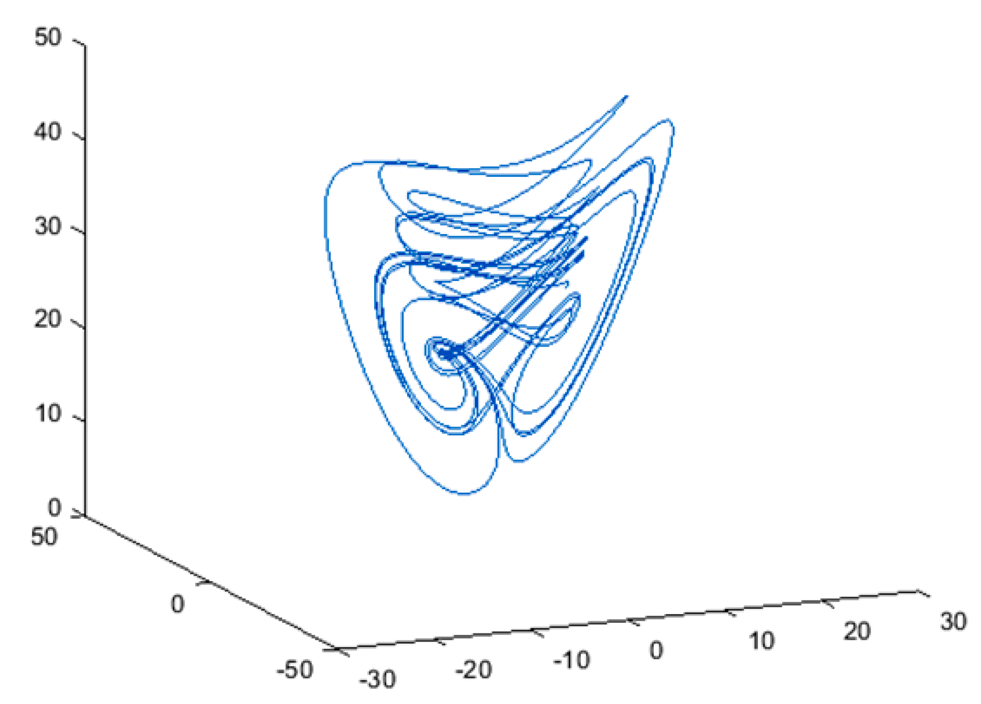
where $x_1$, $x_2$, and $x_3$ are the states (10). The phase portrait of the chaotic Chen system is given in Figure 1.

The time-delay discrete-time chaotic Rossler system is chosen as the slave system. The dynamics of this system are given as follows:

$$\begin{gathered} {\nabla }^{{\alpha }_i} y\left(k+1\right)=f\left(y\left(k\right)\right)-y\left(k\right), \\ {\alpha }_i=1, 2,3 \\ {\alpha }_1=0.9, {\alpha }_2=0.8, {\alpha }_3=0.7 \end{gathered}$$

$$\begin{gathered} y_1\left(k+1\right)-y_1\left(k\right)= \\ \left[\left(-y_2\left(\mathrm{t}-\mathsf{\tau }\right)-y_3\left(\mathrm{t}-\mathsf{\tau }\right)+P_1{I}_1{D}_1+{\mathrm{u}}_1\right)\right]\mathsf{∆} \\ {y}_2\left(k+1\right)-y_2\left(k\right)= \\ \left[\left(y_1\left(\mathrm{t}-\mathsf{\tau }\right)+0.2{\mathrm{y}}_2\left(\mathrm{t}-\mathsf{\tau }\right)\right)+P_2{I}_2{D}_2+{\mathrm{u}}_2\right]\mathsf{∆} \\ {y}_3\left(k+1\right)-y_3\left(k\right)= \\ \left[0.2-5.7y_3\left(\mathrm{t}-\mathsf{\tau }\right)+{\mathrm{y}}_1\left(\mathrm{t}-\mathsf{\tau }\right){\mathrm{y}}_3\left(\mathrm{t}-\mathsf{\tau }\right)+P_3{I}_3{D}_3+{\mathrm{u}}_3\right]\mathsf{∆} \end{gathered}$$

(11)

where $y_1, y_2, and y_3$ are the states of (11). The phase portait of system (11) with $u_i=0$, and $P_i{I}_i{D}_i=0$, $\forall i$ is given in Figure 2.

The synchronization error $e\in {ℝ}^3$ is defined as follows:

$$e_i=y_i\left(\mathrm{t}-\mathsf{\tau }\right)-x_{i }, i=1,2,3$$

(12)

The error dynamics equations are obtained as follows:

$$\begin{gathered} {\nabla }^{{\alpha }_i} e\left(k+1\right)=f\left(e\left(k\right)\right)-e\left(k\right), \\ {\alpha }_1=1, 2,3 \\ {\alpha }_i=0.9, {\alpha }_2=0.8, {\alpha }_3=0.7 \end{gathered}$$

In this paper, we use the discrete-time fractional-order PID controller [13], where $P_i{I}_i{D}_i, i=1, 2, 3$ for each control $u_i, i=1, 2, 3$:

$$\begin{gathered} u_1, u_2, u_3 \\ PID=K_p+K_d{{\displaystyle \sum }}_{k=0}^M{f}_k\left(\mu \right)z^{-k}+K_i\frac{1+z^{-1}}{1+z^{-1}}{{\displaystyle \sum }}_{k=0}^M{f}_k\left(1-\lambda \right)z^{-k} \end{gathered}$$

and $K_p=k_p,K_d=k_d{\alpha }^{\mu },K_i=k_i{\alpha }^{-\lambda }$

$$\begin{gathered} e_1\left(k+1\right)-e_1\left(k\right)= \\ {y}_1\left(k\right)+\left[\left(-y_2\left(\mathrm{t}-\mathsf{\tau }\right)-y_3\left(\mathrm{t}-\mathsf{\tau }\right)+{\mathrm{u}}_1+P_1{I}_1{D}_1\right)\right]\mathsf{∆}-\left\{{\mathrm{x}}_1\left(k\right)+\left[35\left(x_2-{\mathrm{x}}_1\right)\right]\mathsf{∆}\right\}= \\ \left[-(y_1\left(\mathrm{t}-\mathsf{\tau }\right)-x_1)+(y_1\left(\mathrm{t}-\mathsf{\tau }\right)-x_1)-y_2\left(\mathrm{t}-\mathsf{\tau }\right)-y_3\left(\mathrm{t}-\mathsf{\tau }\right)-35x_2+35x_1+u_1+P_1{I}_1{D}_1\right]\mathsf{∆}+ \\ {y}_1\left(k\right)-x_1\left(k\right)= \\ \left[-e_1+(y_1\left(\mathrm{t}-\mathsf{\tau }\right)-x_1)-y_2\left(\mathrm{t}-\mathsf{\tau }\right)-y_3\left(\mathrm{t}-\mathsf{\tau }\right)-35x_2+35x_1+u_1+P_1{I}_1{D}_1 \right]\mathsf{∆}+y_1\left(k\right)-x_1\left(k\right) \end{gathered}$$

(13)

$$\begin{gathered} e_2\left(k+1\right)-e_2\left(k\right)= \\ {y}_2\left(k\right)+\left[y_1\left(\mathrm{t}-\mathsf{\tau }\right)+0.2{\mathrm{y}}_2\left(\mathrm{t}-\mathsf{\tau }\right)+P_2{I}_2{D}_2+{\mathrm{u}}_2\right]\mathsf{∆}-\left\{x_2\left(k\right)+\left[-7x_1-{\mathrm{x}}_1{\mathrm{x}}_3+28x_2\right]\mathsf{∆}\right\}= \\ \{-(y_2\left(\mathrm{t}-\mathsf{\tau }\right)-x_2)+(y_2\left(\mathrm{t}-\mathsf{\tau }\right)-x_2)+\left[y_1\left(\mathrm{t}-\mathsf{\tau }\right)+0.2{\mathrm{y}}_2\left(\mathrm{t}-\mathsf{\tau }\right)+P_2{I}_2{D}_2+u_2+7x_1+{\mathrm{x}}_1{\mathrm{x}}_3-28x_2\right]\}\mathsf{∆}+ \\ {y}_2\left(k\right)-x_2\left(k\right)= \\ \left[-e_2+y_2\left(\mathrm{t}-\mathsf{\tau }\right)-x_{2 }+y_1\left(\mathrm{t}-\mathsf{\tau }\right)+0.2{\mathrm{y}}_2\left(\mathrm{t}-\mathsf{\tau }\right)++P_2{I}_2{D}_2+u_2+7x_1+{\mathrm{x}}_1{\mathrm{x}}_3-28x_2\right]\mathsf{∆}+y_2\left(k\right)-x_2\left(k\right) \end{gathered}$$

$$\begin{gathered} e_3\left(k+1\right)-e_3\left(k\right)= \\ {y}_3\left(k\right)+\left[0.2-5.7y_3\left(\mathrm{t}-\mathsf{\tau }\right)+{\mathrm{y}}_1\left(\mathrm{t}-\mathsf{\tau }\right){\mathrm{y}}_3\left(\mathrm{t}-\mathsf{\tau }\right)+P_3{I}_3{D}_3+{\mathrm{u}}_3\right]\mathsf{∆}-\left[{\mathrm{x}}_3\left(\mathrm{k}\right)+\left(-3x_3+{\mathrm{x}}_1{\mathrm{x}}_2\right)\mathsf{∆}\right]= \\ \{-(y_3\left(\mathrm{t}-\mathsf{\tau }\right)-x_3)+(y_3\left(\mathrm{t}-\mathsf{\tau }\right)-x_3)+ \\ 0.2-5.7y_3\left(\mathrm{t}-\mathsf{\tau }\right)+{\mathrm{y}}_1\left(\mathrm{t}-\mathsf{\tau }\right){\mathrm{y}}_3\left(\mathrm{t}-\mathsf{\tau }\right)+P_3{I}_3{D}_3+{\mathrm{u}}_3+3x_3-{\mathrm{x}}_1{\mathrm{x}}_2\}\mathsf{∆}+y_3\left(k\right)-x_3\left(k\right)= \\ -e_3+(y_3\left(\mathrm{t}-\mathsf{\tau }\right)-x_3)+ \\ 0.2-5.7y_3\left(\mathrm{t}-\mathsf{\tau }\right)+{\mathrm{y}}_1\left(\mathrm{t}-\mathsf{\tau }\right){\mathrm{y}}_3\left(\mathrm{t}-\mathsf{\tau }\right)+P_3{I}_3{D}_3+{\mathrm{u}}_3+3x_3-{\mathrm{x}}_1{\mathrm{x}}_2\}\mathsf{∆}+y_3\left(k\right)-x_3\left(k\right) \end{gathered}$$

We need to find the nonlinear active control law for $u_i$, $\forall i$, in such a manner that the error dynamics of (13) are globally asymptotically stable. Let

$$\begin{gathered} u_1=(-y_1\left(\mathrm{t}-\mathsf{\tau }\right)+x_1)+y_2\left(\mathrm{t}-\mathsf{\tau }\right)+y_3\left(\mathrm{t}-\mathsf{\tau }\right)+35x_2-35x_1-P_1{I}_1{D}_1 \\ {u}_2=-y_2\left(\mathrm{t}-\mathsf{\tau }\right)+x_2-y_1\left(\mathrm{t}-\mathsf{\tau }\right)-0.2{\mathrm{y}}_2\left(\mathrm{t}-\mathsf{\tau }\right)-P_2{I}_2{D}_2-7x_1-{\mathrm{x}}_1{\mathrm{x}}_3+28x_2 \\ {u}_3=(-y_3\left(\mathrm{t}-\mathsf{\tau }\right)+x_3)-0.2+5.7y_3\left(\mathrm{t}-\mathsf{\tau }\right)-{\mathrm{y}}_1\left(\mathrm{t}-\mathsf{\tau }\right){\mathrm{y}}_3\left(\mathrm{t}-\mathsf{\tau }\right)-P_3{I}_3{D}_3-3x_3+{\mathrm{x}}_1{\mathrm{x}}_2 \end{gathered}$$

(14)

Substituting the controller dynamics (14) into the error dynamics (13), we have error dynamics as follows:

$$\begin{gathered} e_1\left(k+1\right)-e_1\left(k\right)=\left[-e_1\right]∆+y_1\left(k\right)-x_1\left(k\right) \\ {e}_2\left(k+1\right)-e_2\left(k\right)=\left[-e_2\right]∆+y_2\left(k\right)-x_2\left(k\right) \\ {e}_3\left(k+1\right)-e_3\left(k\right)=\left[-e_3\right]∆+y_3\left(k\right)-x_3\left(k\right) \\ {e}_1\left(k+1\right)-e_1\left(k\right)=\left[-e_1\right]∆+e_1 \\ {e}_2\left(k+1\right)-e_2\left(k\right)=\left[-e_2\right]∆+e_2 \\ {e}_3\left(k+1\right)-e_3\left(k\right)=\left[-e_3\right]∆+e_3 \end{gathered}$$

(15)

The synchronization problem is used to determine the nonlinear controller $U$ so that:

$$\underset{t\to \infty }{\lim }\parallel e\left(t\right)\parallel =0$$

To show that the previous limit is satisfied, we make use of the positive definite Lyapunov–Krasovskii function as follows [14,15,16]:

$$V\left(e\right)=\frac{1}{2}\left(e_1^2+e_2^2+e_3^2\right)+{{\displaystyle \int }}_{t-\tau }^{t}g\left(x\left(\zeta \right)\right)d\zeta$$

(16)

The Lyapunov–Krasovskii function is defined for systems that are continuous in time, and for discrete systems, as in our case study, the integral in (16) is replaced by the following summation, and the function thus obtained is called the Lyapunov–Krasovskii function for discrete systems in time:

$$V_1\left(e_t\right)={\displaystyle \sum }_{i=t-h}^{t-1}{e}^T\left(i\right)Qe\left(i\right)$$

Here, we use the known inequality in fractional order systems as follows:

$$\frac{1}{2}{}_{t_0}{}^{C}D{}_t^{\alpha }{e}_{\mathrm{k}}{}^2\left(t\right)\le e{\left(t\right)}_{t_0}^C{D}_t^{\alpha }e\left(t\right),\forall \alpha \in \left(0,1\right)$$

Assuming first-order partial derivatives of (16) exist, using the procedure in (7), we have

$$∆\left(V\left(e\right)\right)=e_1{\dot{e}}_1+e_2{\dot{e}}_2+e_3{\dot{e}}_3+e^T\left(t\right)Qe\left(t\right)-e^T\left(t-h\right)Qe\left(t-h\right)$$

(17)

Substituting (15) into (17), we obtain

$$\begin{gathered} ∆\left(V\left(e\right)\right)=-e_1^2\mathsf{∆}+{\mathrm{e}}_1^2-e_2^2\mathsf{∆}+{\mathrm{e}}_2^2-e_3^2\mathsf{∆}+{\mathrm{e}}_3^2+e^T\left(t\right)Qe\left(t\right)-e^T\left(t-h\right)Qe\left(t-h\right) \\ ∆\left(V\left(e\right)\right)=-e_1^2\mathsf{∆}+\parallel {\mathrm{e}}_1\parallel -e_2^2\mathsf{∆}+\parallel {\mathrm{e}}_2\parallel -e_3^2\mathsf{∆}+\parallel {\mathrm{e}}_3\parallel + \\ \parallel e\left(t-h\right)\parallel \end{gathered}$$

(18)

$$∆\left(V\left(e\right)\right)=-e_1^2\mathsf{∆}-e_2^2\mathsf{∆}-e_3^2\mathsf{∆}<0)$$

where $∆\left(V\left(e\right)\right)$ is a negative definite. For the Lyapunov stability theory, the error dynamics (15) are globally asymptotically stable and will converge to zero as $t\to \infty$ with the control law in (14). The Chen (10) and Rossler (11) chaotic systems are globally asymptotically synchronized for any initial condition.

The analytical results obtained through the examples developed by simulation are illustrated below for sinchronization.

The Chen and Rossler systems were simulated in Simulink in MATLAB using the control law $U$ (14) for synchronization. The initial conditions for these systems are $x\left(0\right)={\left[-10, 0, 37\right]}^T$ and $y\left(0\right)={\left[0.1, 0, 0\right]}^T$, and similarly for the simulation.

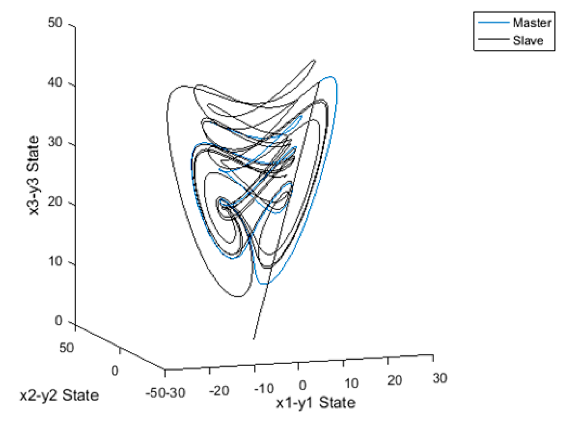
The time evolution of the states of the Chen and Rossler systems for synchronization with time delayed is shown in Figure 3, Figure 4 and Figure 5.

For these simulations, we used $∆=0.001$ and $\tau =20 s.$

Synchronization errors of states are shown in Figure 6.

5. Anti-Synchronization of Variable-Order Fractional Discrete-Time Chen and Rossler Chaotic Systems

In this section, we solve the problem of anti-synchronization of the discrete-time Chen and Rossler systems, considered as master and slave, respectively. The discrete-time Chen system dynamics are given as follows:

The discrete-time anti-synchronization error $e_{as}\in {ℝ}^3$ is defined as follows:

$$e_{a{s}_i}=Y_s+X_m, i=1, 2, 3$$

(19)

From (1), (2), and (19), the dynamics of the error are as follows:

$$\begin{gathered} {\dot{e}}_{as}={\dot{Y}}_s+{\dot{X}}_m= \\ [Y_s\left(k+1\right)-Y_s\left(k\right)]+\left[X_m\left(k+1\right)-X_m\left(k\right)\right]= \\ \left\{\left[Q\left(Y_s\right)+g\left(Y_s\right)+U\right]+\left[ P\left(X_m\right)+f\left(X_m\right)\right]\right\}\mathsf{∆} \end{gathered}$$

The anti-synchronization problem is used to determine the nonlinear control $U$ that satisfies $\underset{t\to \infty }{\lim }\parallel e\left(t\right)\parallel =0$, $\forall e_{a{s}_i}\left(t\right)\in {ℝ}^n$.

Consider a positive definite Lyapunov function, as follows:

$$V\left({\mathrm{e}}_{{\mathrm{as}}_{\mathrm{i}}}\right)=\frac{1}{2}{\displaystyle \sum }_{\mathrm{k}=1}^{\mathrm{n}}{e}_{a{s}_k}^2$$

and using the procedure in (7), we have the following:

$$\begin{gathered} ∆\left(V\left({\mathrm{e}}_{\mathrm{as}}\right)\right)=[{\displaystyle \sum }_{\mathrm{k}=1}^{\mathrm{n}}{\mathrm{e}}_{\mathrm{as}}{}_{\mathrm{k}}{\mathrm{ė}}_{\mathrm{as}}{}_{\mathrm{k}}] \\ \frac{1}{2}{}_{t_0}{}^{C}D{}_t^{\alpha }{\mathrm{e}}_{\mathrm{a}}{{}_{\mathrm{s}}}_{\mathrm{k}}{}^2\left(t\right)\le e{\left(t\right)}_{t_0}^C{D}_t^{\alpha }{\mathrm{e}}_{\mathrm{a}}{{}_{\mathrm{s}}}_{\mathrm{k}}{}^2\left(t\right),\forall \alpha \in \left(0,1\right), \end{gathered}$$

With $V\left({\mathrm{e}}_{\mathrm{as}}\right)\to \infty$ as $\parallel {\mathrm{e}}_{\mathrm{as}}\left(\mathrm{t}\right)\parallel \to \infty$, $e_{as}$ is globally asymptotically stable, and the states and response systems are globally asymptotically synchronized.

The discrete-time Chen and Rossler systems are considered as master and slave, respectively. The discrete-time Chen system dynamics are given as follows:

$$\begin{gathered} {\nabla }^{{\alpha }_i} x\left(k+1\right)=f\left(x\left(k\right)\right)-x\left(k\right), \\ {\alpha }_i=1, 2,3 \\ {\alpha }_1=0.9, {\alpha }_2=0.8, {\alpha }_3=0.7 \end{gathered}$$

$$\begin{gathered} x_1\left(k+1\right)-x_1\left(k\right)=\left[35\left(x_2-{\mathrm{x}}_1\right)\right]\mathsf{∆} \\ {x}_2\left(k+1\right)-x_2\left(k\right)=\left(-7x_1-{\mathrm{x}}_1{\mathrm{x}}_3+28x_2\right)\mathsf{∆} \\ {x}_3\left(k+1\right)-x_3\left(k\right)=\left(-3x_3+{\mathrm{x}}_1{\mathrm{x}}_2\right)\mathsf{∆} \end{gathered}$$

where $x_1$, $x_2$, and $x_3$ are the states (10).

The discrete-time Rossler chaotic system is chosen as the slave system. The dynamics of this system are given as follows:

$$\begin{gathered} {\nabla }^{{\alpha }_i} y\left(k+1\right)=f\left(y\left(k\right)\right)-y\left(k\right), \\ {\alpha }_i=1, 2,3 \\ {\alpha }_1=0.9, {\alpha }_2=0.8, {\alpha }_3=0.7 \end{gathered}$$

$$\begin{gathered} y_1\left(k+1\right)-y_1\left(k\right)=\left[\left(-y_2\left(t-\tau \right)-y_3\left(t-\tau \right)+P_1{I}_1{D}_1+u_1\right)\right]∆ \\ {y}_2\left(k+1\right)-y_2\left(k\right)=\left[\left(y_1\left(t-\tau \right)+0.2y_2\left(t-\tau \right)\right)+P_2{I}_2{D}_2+u_2\right]∆ \\ {y}_3\left(k+1\right)-y_3\left(k\right)=\left[0.2-5.7y_3\left(t-\tau \right)+y_1\left(t-\tau \right)y_3\left(t-\tau \right)+P_3{I}_3{D}_3+u_3\right]∆ \end{gathered}$$

where $y_1, y_2, and y_3$ are the states of the system (11). The phase plane for system (11) with $u_i=0$ and $P_i{I}_i{D}_i=0$ $\forall i$, where $u_1, u_2, and u_3$ are the active nonlinear controllers to be designed.

The anti-synchronization error $e\in {ℝ}^3$ is defined as follows:

$$e_{a{s}_i}=y_i\left(\mathrm{t}-\mathsf{\tau }\right)+{\mathrm{u}}_{\mathrm{i}}+x_{i }, i=1,2,3$$

The error dynamics equations are obtained as follows:

$$\begin{gathered} {\nabla }^{{\alpha }_i} e_{a{s}_i}\left(k+1\right)=f\left(e_{a{s}_i}\left(k\right)\right)-e_{a{s}_i}\left(k\right), \\ {\alpha }_i=1, 2,3 \\ {\alpha }_1=0.9, {\alpha }_2=0.8, {\alpha }_3=0.7 \end{gathered}$$

$$\begin{gathered} e_{a{s}_1}\left(k+1\right)-e_{a{s}_1}\left(k\right)=y_1\left(k\right)+\left[\left(-y_2\left(t-\tau \right)-y_3\left(t-\tau \right)+u_1+P_1{I}_1{D}_1\right)\right]∆ \\ +\left\{x_1\left(k\right)+\left[35\left(x_2-x_1\right)\right]∆\right\}= \\ \left[-(y_1\left(t-\tau \right)+x_1)+(y_1\left(t-\tau \right)+x_1)-y_2\left(t-\tau \right)-y_3\left(t-\tau \right)+35x_2-35x_1+u_1+P_1{I}_1{D}_1\right]∆+ \\ {y}_1\left(k\right)+x_1\left(k\right)= \\ \left[-e_1+(y_1\left(t-\tau \right)+x_1)-y_2\left(t-\tau \right)-y_3\left(t-\tau \right)+35x_2-35x_1+u_1+P_1{I}_1{D}_1 \right]∆+ \\ {y}_1\left(k\right)+x_1\left(k\right) \end{gathered}$$

(20)

$$\begin{gathered} e_{a{s}_2}\left(k+1\right)-e_{a{s}_2}\left(k\right)=y_2\left(k\right)+\left[y_1\left(t-\tau \right)+0.2y_2\left(t-\tau \right)+P_2{I}_2{D}_2+u_2\right]∆ \\ +\left\{x_2\left(k\right)+\left[-7x_1-x_1{x}_3+28x_2\right]∆\right\}= \\ \{-(y_2\left(t-\tau \right)+x_2)+(y_2\left(t-\tau \right)+x_2)+\left[y_1\left(t-\tau \right)+0.2y_2\left(t-\tau \right)+P_2{I}_2{D}_2+u_2-7x_1-x_1{x}_3+28x_2\right]\}∆+ \\ {y}_2\left(k\right)+x_2\left(k\right)= \\ \left[-e_2+y_2\left(t-\tau \right)+x_{2 }+y_1\left(t-\tau \right)+0.2y_2\left(t-\tau \right)++P_2{I}_2{D}_2+u_2-7x_1-x_1{x}_3+28x_2\right]∆+ \\ {y}_2\left(k\right)+x_2\left(k\right) \end{gathered}$$

$$\begin{gathered} e_{a{s}_3}\left(k+1\right)-e_{a{s}_3}\left(k\right)= \\ {y}_3\left(k\right)+\left[0.2-5.7y_3\left(t-\tau \right)+y_1\left(t-\tau \right)y_3\left(t-\tau \right)+P_3{I}_3{D}_3+u_3\right]∆+\left[x_3\left(k\right)+\left(-3x_3+x_1{x}_2\right)∆\right]= \\ \{-(y_3\left(t-\tau \right)+x_3)+(y_3\left(t-\tau \right)+x_3)+ \\ 0.2-5.7y_3\left(t-\tau \right)+y_1\left(t-\tau \right)y_3\left(t-\tau \right)+P_3{I}_3{D}_3+u_3-3x_3+x_1{x}_2\}∆+y_3\left(k\right)+x_3\left(k\right)= \\ \left[-e_3+(y_3\left(t-\tau \right)+x_3\right)+ \\ 0.2-5.7y_3\left(t-\tau \right)+y_1\left(t-\tau \right)y_3\left(t-\tau \right)+P_3{I}_3{D}_3+u_3-3x_3+x_1{x}_2\}∆+ \\ {y}_3\left(k\right)+x_3\left(k\right) \end{gathered}$$

We need to find the nonlinear active control law for $u_i$, $\forall i$, such that the error dynamics of (13) are globally asymptotically stable. Let

$$\begin{gathered} u_1=(-y_1\left(t-\tau \right)-x_1)+y_2\left(t-\tau \right)+y_3\left(t-\tau \right)-35x_2+35x_1+u_1-P_1{I}_1{D}_1 \\ {u}_2=-y_2\left(t-\tau \right)-x_2-y_1\left(t-\tau \right)-.2y_2\left(t-\tau \right)-P_2{I}_2{D}_2+7x_1+x_1{x}_3-28x_2 \\ {u}_3=(-y_3\left(t-\tau \right)-x_3)-0.2+5.7y_3\left(t-\tau \right)-y_1\left(t-\tau \right)y_3\left(t-\tau \right)-P_3{I}_3{D}_3+3x_3-x_1{x}_2\} \end{gathered}$$

(21)

Substituting the controller dynamics (21) into the error dynamics (20), we have error dynamics, as follows:

$$\begin{gathered} e_{a{s}_1}\left(k+1\right)-e_{a{s}_1}\left(k\right)=\left[-e_{a{s}_1}\right]∆+y_1\left(k\right)+x_1\left(k\right) \\ {e}_{a{s}_2}\left(k+1\right)-e_{a{s}_2}\left(k\right)=\left[-e_{a{s}_2}\right]∆+y_2\left(k\right)+x_2\left(k\right) \\ {e}_{a{s}_3}\left(k+1\right)-e_{a{s}_3}\left(k\right)=\left[-e_{a{s}_3}\right]∆+y_3\left(k\right)+x_3\left(k\right) \end{gathered}$$

$$\begin{gathered} e_{a{s}_1}\left(k+1\right)-e_{a{s}_1}\left(k\right)=\left[-e_{a{s}_1}\right]∆+e_{a{s}_1} \\ {e}_{a{s}_2}\left(k+1\right)-e_{a{s}_2}\left(k\right)=\left[-e_{a{s}_2}\right]∆+e_{a{s}_2} \\ {e}_{a{s}_3}\left(k+1\right)-e_{a{s}_3}\left(k\right)=\left[-e_{a{s}_3}\right]∆+e_{a{s}_3} \end{gathered}$$

(22)

The synchronization problem is to determine the nonlinear controller $U$, so that:

$$\underset{t\to \infty }{\lim }\parallel e\left(t\right)\parallel =0$$

Considering a positive definite Lyapunov function, as follows [14,15,16]:

$$V\left(e_{as}\right)=\frac{1}{2}\left(e_{a{s}_1}^2+e_{a{s}_2}^2+e_{a{s}_3}^2\right)+{{\displaystyle \int }}_{t-\tau }^{t}g\left(x\left(\zeta \right)\right)d\zeta$$

The Lyapunov–Krasovskii function is defined for systems that are continuous in time, and for discrete systems, as in our case study, the integral is replaced by the following summation, and the function thus obtained is called the Lyapunov–Krasovskii function for discrete systems in time.

$$\begin{gathered} V_1\left(e_t\right)={\displaystyle \sum }_{i=t-h}^{t-1}{e}^T\left(i\right)Qe\left(i\right) \\ V\left(e_{as}\right)=\frac{1}{2}\left(e_{a{s}_1}^2+e_{a{s}_2}^2+e_{a{s}_3}^2\right)+{\displaystyle \sum }_{i=t-h}^{t-1}{e}^T\left(i\right)Qe\left(i\right) \end{gathered}$$

(23)

Assuming first-order partial derivatives of (23) exist, we use the procedure in (7), as follows:

$$∆\left(V\left(e_{a{s}_1}\right)\right)=e_{a{s}_1}{\dot{e}}_{a{s}_1}+e_{a{s}_2}{\dot{e}}_{a{s}_2}+e_{a{s}_3}{\dot{e}}_{a{s}_3}+e^T\left(t\right)Qe\left(t\right)-e^T\left(t-h\right)Qe\left(t-h\right)$$

(24)

Substituting (22) into (24), we obtain

$$\begin{gathered} ∆\left(V\left(e_{as}\right)\right)=-e_{a{s}_1}^2\mathsf{∆}+e_{a{s}_1}^2-e_{a{s}_2}^2\mathsf{∆}+e_{a{s}_2}^2-e_{a{s}_3}^2\mathsf{∆}+e_{a{s}_3}^2+e^T\left(t\right)Qe\left(t\right)-e^T\left(t-h\right)Qe\left(t-h\right) \\ ∆\left(V\left(e_{as}\right)\right)=-e_{a{s}_1}^2\mathsf{∆}+\parallel e_{a{s}_2}\parallel -e_{a{s}_3}^2\mathsf{∆}+\parallel e_{a{s}_3}\parallel -e_{a{s}_3}^2∆+\parallel e_{a{s}_3}\parallel +\parallel e_{a{s}_3}\parallel + \\ \parallel e\left(t-h\right)\parallel \\ ∆\left(V\left(e_{as}\right)\right)=-e_{a{s}_1}^2\mathsf{∆}-e_{a{s}_2}^2\mathsf{∆}-e_{a{s}_3}^2\mathsf{∆} \end{gathered}$$

(25)

where $∆\left(V\left(e\right)\right)$ is a negative definite. For the Lyapunov stability theory, the error dynamics (22) are globally asymptotically stable and the error dynamics will converge to zero as $t\to \infty$ with the control law in (21). The Chen (10) and Rossler (11) chaotic systems are globally asymptotically anti-synchronized for any initial condition, and with this analysis, we have the next theorem.

The analytical results obtained through examples developed by simulation are illustrated below for anti-synchronization.

The Chen and Rossler systems were simulated in Simulink in MATLAB using the control law $U$ (21) for anti-synchronization.

The initial conditions for these systems are $x\left(0\right)={\left[-10, 0, 37\right]}^T$ and $y\left(0\right)={\left[0.1, 0, 0\right]}^T$, and similarly for the simulation.

The evolution over the time of the states of the Chen and Rossler systems for anti-synchronization is shown in Figure 7, Figure 8 and Figure 9.

For these simulations, we used $∆=0.001$ and $\tau =20 s.$

Anti-synchronization errors of states are shown in Figure 10.

Theorem 1.

The synchronization and anti-sinchronization problem of discrete fractional-order chaotic systems in time is solved by means of control laws (14) and (21), which are obtained using the stability analysis through the Lyapunov–Krasovskii and PID control laws for fractional-order systems, so we ensure that$∆\left(V\left(e\right)\right)<0$ $\forall e\ne 0$, and then$\underset{k\to \infty }{\lim }e\left(k\right)=0$,$∆\left(V\left(e_{as}\right)\right)<0$ $\forall e_{as}\ne 0$, and then$\underset{k\to \infty }{lim} e_{as}\left(k\right)=0$; therefore, the synchronization and anti-synchronization problem is solved.

6. Conclusions

In this research work, a solution is given to the problem of the synchronization and anti-synchronization of chaotic systems described by differential equations of a variable order derivative and discrete time with a time delay. The problem is solved by means of a control law, which is deduced by the well-known discrete Lyapunov–Krasovskii stability analysis and discrete PID control laws, as can be seen in the simulations in Section 4 and Section 5. The analytical results obtained are illustrated by simulations; as can be seen, the results are satisfactory. These simulations were carried out in the Simulink-MATLAB environment.

Remarks:

Although the study that was carried out was for Chen and Rossler chaotic systems of a variable fractional order with time delay, the methodology can be used for other chaotic or hyperchaotic systems, or other types of systems.

References

1. Bendoukha, S.; Ouannas, A.; Wang, X.; Khennaoui, A.A.; Pham, V.T.; Grassi, G.; Huynh, V.V. The Co-existence of Different Synchronization Types in Fractional-order Discrete-time Chaotic Systems with Non–identical Dimensions and Orders. Entropy 2018, 20, 710. [Google Scholar] [CrossRef] [PubMed] [Green Version]
2. Zhang, R.; Chen, D.; Do, Y.; Ma, X. Synchronization and anti-synchronization of fractional dynamical networks. J. Vib. Control. 2015, 21, 3383–3402. [Google Scholar] [CrossRef]
3. Sierociuk, D.; Malesza, W. Fractional variable order discrete-time systems, their solutions and properties. Int. J. Syst. Sci. 2017, 48, 3098–3105. [Google Scholar] [CrossRef]
4. Zhang, W.; Cao, J.; Alsaedi, A.; Alsaadi, F.E.S. Synchronization of Time Delayed Fractional Order Chaotic Financial System. Hindawi Discret. Dyn. Nat. Soc. 2017, 2017, 1230396. [Google Scholar] [CrossRef] [Green Version]
5. Ostalczyk, P. Variable-, fractional-order discrete PID controllers, 2012. In Proceedings of the 17th International Conference on Methods Models in Automation Robotics (MMAR), Miedzyzdroje, Poland, 27–30 August 2012; pp. 534–539. [Google Scholar] [CrossRef]
6. Jiang, H.P.; Liu, Y.Q. Disturbance Rejection for Fractional-Order Time-Delay Systems. Hindawi Publ. Corp. Math. Probl. Eng. 2016, 2016, 1316046. [Google Scholar] [CrossRef]
7. Wu, G.C.; Deng, Z.G.; Baleanu, D.; Zeng, D.Q. New variable-order fractional chaotic systems for fast image encryption. Chaos 2019, 29, 083103. [Google Scholar] [CrossRef] [PubMed]
8. Baleanu, D.; Wu, G.C.; Bai, Y.R.; Chen, F.L. Stability analysis of Caputo–like discrete fractional systems. Commun. Nonlinear Sci. Numer. Simulat. 2017, 48, 520–530. [Google Scholar] [CrossRef]
9. Yousefi, F.S.; Ordokhani, Y. Numerical solution of variable-order fractional differential equations by Legendre cardinal functions. In Proceedings of the 4th International Conference on Combinatorics, Cryptography, Computer Science and Computing, Iran University of Science Technology, Tehran City, Iran, 20–21 November 2019. [Google Scholar]
10. Djennoune, S.; Bettayeb, M.; Al-Saggaf, U.M. Synchronization of Fractional-Order Discrete-Time Chaotic Systems by An Exact Delayed State Reconstructor: Applications To Secure Communication. Int. J. Appl. Math. Comput. Sci. 2019, 29, 179–194. [Google Scholar] [CrossRef] [Green Version]
11. Aguila-Camacho, N.; Duarte-Mermoud, M.A.; Gallegos, J.A. Lyapunov functions for fractional order systems. Commun. Nonlinear Sci. Numer. Simulat. 2014, 19, 2951–2957. [Google Scholar] [CrossRef]
12. Wei, Y.; Chen, Y.; Liu, T.; Wang, Y. Lyapunov functions for nabla discrete fractional order systems. ISA Trans. 2019, 88, 82–90. [Google Scholar] [CrossRef] [PubMed]
13. Merrikh-Bayat, F.; Mirebrahimi, N.; Khalili, M.R. Discrete-Time Fractional-Order PID Controller: Definition, Tuning, Digital Realization and Some Applications. Int. J. Control. Autom. Syst. 2015, 13, 81–90. [Google Scholar] [CrossRef]
14. Hu, J.B.; Zhao, L.D.; Lu, G.P.; Zhang, S.B. The stability and control of fractional nonlinear system with distributed time delay. Appl. Math. Model. 2016, 40, 3257–3263. [Google Scholar] [CrossRef]
15. Seuret, A.; Fridman, E. Wirtinger-like Lyapunov–Krasovskii functionals for discrete-time delay systems. IMA J. Math. Control. Inf. 2018, 35, 861–876. [Google Scholar] [CrossRef]
16. Stojanović, S.B.; Debeljković, D.L.; Mladenović, I. A Lyapunov-Krasovskii Methodology for Asymptotic Stability of Discrete Time Delay Systems. Servian J. Electr. Eng. 2007, 4, 109–117. [Google Scholar] [CrossRef]
Figure 1. Phase portrait of discrete-time chaotic Chen system.
Mathematics 09 02149 g001
Figure 2. Phase portrait of discrete-time chaotic Rossler system.
Mathematics 09 02149 g002
Figure 3. Time response (ac) of synchronized states of master and slave.
Mathematics 09 02149 g003
Figure 4. Phase space of synchronization of original master–slave system.
Mathematics 09 02149 g004
Figure 5. Phase space of synchronization of master–slave system with fractional order given by c = 0.9, c1 = 0.8, c2 = 0.7.
Mathematics 09 02149 g005
Figure 6. Synchronization errors with time delay between states of master and slave system of variable fractional order derivative.
Mathematics 09 02149 g006
Figure 7. Time response (ac) of synchronized states of master and slave.
Mathematics 09 02149 g007
Figure 8. Phase space of anti-synchronization of an original master–slave system.
Mathematics 09 02149 g008
Figure 9. Phase space of anti-synchronization of master–slave systems with fractional orders given by c = 0.9, c1 = 0.8, and c2 = 0.7.
Mathematics 09 02149 g009
Figure 10. Anti-synchronization errors with time delay between states of master and slave systems of a variable fractional-order derivative.
Mathematics 09 02149 g010
Publisher’s Note: MDPI stays neutral with regard to jurisdictional claims in published maps and institutional affiliations.