Isometry Invariant Shape Recognition of Projectively Perturbed Point Clouds by the Mergegram Extending 0D Persistence ^†

Abstract

Rigid shapes should be naturally compared up to rigid motion or isometry, which preserves all inter-point distances. The same rigid shape can be often represented by noisy point clouds of different sizes. Hence, the isometry shape recognition problem requires methods that are independent of a cloud size. This paper studies stable-under-noise isometry invariants for the recognition problem stated in the harder form when given clouds can be related by affine or projective transformations. The first contribution is the stability proof for the invariant mergegram, which completely determines a single-linkage dendrogram in general position. The second contribution is the experimental demonstration that the mergegram outperforms other invariants in recognizing isometry classes of point clouds extracted from perturbed shapes in images.

1. Introduction: Motivations, Shape Recognition Problem, and Overview of Results

Real-life objects are often represented by unstructured point clouds obtained by laser range scanning or by selecting salient or feature points in images [1]. Point clouds are easy to store and can be used as primitives for visualization [2]. The above advantages strongly motivate the problem of comparing and classifying unstructured point clouds.

Rigid objects are naturally studied up to rigid motion or isometry (including reflections), which is any map that preserves inter-point distances. The recognition of point clouds of the same number of points is practically solved by the histogram of all pairwise distances, which is a complete isometry invariant in general position [3].

Real shapes are often given in a distorted form because of noisy measurements, when points are perturbed, missed or accidentally added. One of the first approaches to recognize nearly identical point clouds $A,B$ of different sizes in the same metric space, for example, in ${\mathbb{R}}^m$, is to use the Hausdorff distance [4] $\mathrm{HD}(A,B)=min{ϵ}^{\ge }0$ such that the first cloud A is covered by ${ϵ}^{}-balls centered at all points of$B$, and vice versa.$

However, we also need to take into account infinitely many potential isometries of the ambient space ${\mathbb{R}}^m$. The exact computation of ${inf}_f\mathrm{HD}(f\left(A\right),B)$ minimized over isometries f of ${\mathbb{R}}^m$ has a high polynomial complexity already for dimension $m=2$ [5]. An approximate algorithm is cubic in the number of points for $m=3$ [6].

This paper extends the 12-page conference version [7], which introduced the new invariant mergegram but did not prove its continuity under perturbations. In addition to the proof of continuity, another contribution is Theorem 2 showing how to reconstruct a dendrogram of single-linkage clustering from a mergegram in general position.

The practical novelty is the harder recognition problem including perturbations of isometries within wider classes of affine and projective maps motivated by computer vision applications. Indeed, different positions of cameras produce projectively equivalent images of the same rigid shape. The new experiments in Section 6 extensively compared several approaches on 15,000 clouds obtained from real images; see examples in Figure 1.

Problem 1

(isometry shape recognition under noise). Find an isometry invariant of point clouds in ${\mathbb{R}}^m$ that is (a) independent of a cloud size, (b) provably continuous under perturbations of a cloud, (c) computable in a near linear time in the size of a cloud, and (d) more efficient for recognizing isometry classes of clouds than past invariants.

The key contributions are Theorems 2 and 3 and the experiments in Section 6 showing that the mergegram achieves a state-of-the-art recognition on substantially distorted images.

2. Related Work on Isometry Shape Recognition and Topological Data Analysis

For the isometry classification of clouds consisting of the same number of points, the easiest invariant is the distribution of all pairwise distances, whose completeness (or injectivity) was proved for all point clouds in general (non-singular) position in ${\mathbb{R}}^m$ [3].

Fixed point clouds $A,B\subset {\mathbb{R}}^m$ of different sizes can be pairwisely compared by the Hausdorff distance [4] $\mathrm{HD}(A,B)=max\{\underset{p\in A}{sup}{d}_B\left(p\right),\underset{q\in B}{sup}{d}_A\left(q\right)\}$, where $d_B\left(p\right)=\underset{q\in B}{inf}d(p,q)$ is the (Euclidean or another) distance from a point $p\in A$ to the cloud B.

The rigid shape recognition problem for non-fixed clouds $A,B$ is harder because of infinitely many potential isometries that can match $A,B$ exactly or approximately. Partial cases of this problem were studied for clouds representing surfaces [10] and when two clouds have a given isometric matching of one pair of points [11]. Shape Google by Ovsjanikov et al. practically extends these ideas to non-rigid shape recognition [12].

The most general framework for the isometry shape recognition of point cloud data was proposed by Mémoi and Sapiro [13]. They studied the Gromov-Hausdorff distance $d_{GH}(A,B)=\underset{f,g,M}{inf}\mathrm{HD}(f\left(A\right),g\left(B\right))$ minimized over all isometric embeddings $f:A\to M$ and $g:B\to M$ of given point clouds into a metric space M. Since the above definitions involve even more minimizations over infinitely many maps and spaces, $\mathrm{GH}$ can be only approximated. The Farthest Point Sampling (FPS) has a quadratic complexity in the number of points (Reference [13], Section 3.6) and was successfully tested on small clouds.

The proposed invariant mergegram extends the 0-dimensional persistence in the area of Topological Data Analysis (TDA), which grew from the theory of size functions [14]. TDA views a point cloud $A\subset {\mathbb{R}}^m$ not by fixing any distance threshold but across all scales s, for example, by blurring given points of A to balls of a variable radius s. The evolution of this growing union of balls is summarized by a persistence diagram, which is invariant under isometries of ${\mathbb{R}}^m$. TDA can be combined with machine learning and statistical tools due to stability under noise, which was first proved by Cohen-Steiner et al. [15] and then extended to a very general form by Chazal et al. [16].

In dimension 0 the persistence diagram $\mathrm{PD}\left(A\right)$ for distance-based filtrations of a point cloud A consists of the pairs $(0,s)\in {\mathbb{R}}^2$, where values of s are distance scales at which subsets of A merge by the single-linkage clustering. These scales equal half-lengths of edges in a Minimum Spanning Tree $\mathrm{MST}\left(A\right)$. If distances between all points of A are known, $\mathrm{MST}\left(A\right)$ is a connected graph with the vertex set A and a minimal total length.

Representing a point cloud A by $\mathrm{PD}\left(A\right)$ loses a lot of geometry of A, but gains stability under perturbations, which can be expressed in the case of point clouds as $\mathrm{BD}\left(\mathrm{PD}\right(A),\mathrm{PD}(B\left)\right)\le \mathrm{HD}(A,B)$. Here, the bottleneck distance $\mathrm{BD}$ between diagrams is defined as a minimum ${ϵ}^{\ge }0$ such that all pairs of $\mathrm{PD}\left(A\right)$ can be bijectively matched to ${ϵ}^{}-close points of$ PD(B) $or to diagonal pairs$ (s,s) $, and vice versa . Here,$-closeness of pairs $(a,c)$ and $(b,d)$ in ${\mathbb{R}}^2$ is measured in the distance $L_{\infty }=max\left\{\right|a-b|,|c-d\left|\right\}$.

The mergegram extends $\mathrm{PD}\left(A\right)$ to a stronger invariant, whose stability under perturbations in the above sense is proved in Section 5 for the first time. The idea of a mergegram is related to the Reeb graph [17] or the merge tree [18] for the sublevel set filtration of a scalar function. The mergegram $\mathrm{MG}$ is defined at a more abstract level for any clustering dendrogram, which opens a possibility to extend a Homologically Persistent Skeleton (HoPeS) visualizing most persistent cycles in point clouds [19].

Since any persistence diagram and a mergegram are unordered collections of pairs, the experiments in Section 6 use the neural network PersLay [20], whose output is invariant under permutations of input points by design. PersLay extends the neural network DeepSet [21] and introduces new layers to accept as an input any diagram of unordered points. In other related work, deep learning was recently applied to outputs of hierarchical clustering [22,23,24] and to 0-dimensional persistence [25,26].

3. Single-Linkage Clustering and the Invariant Mergegram of a Dendrogram

Example 1.

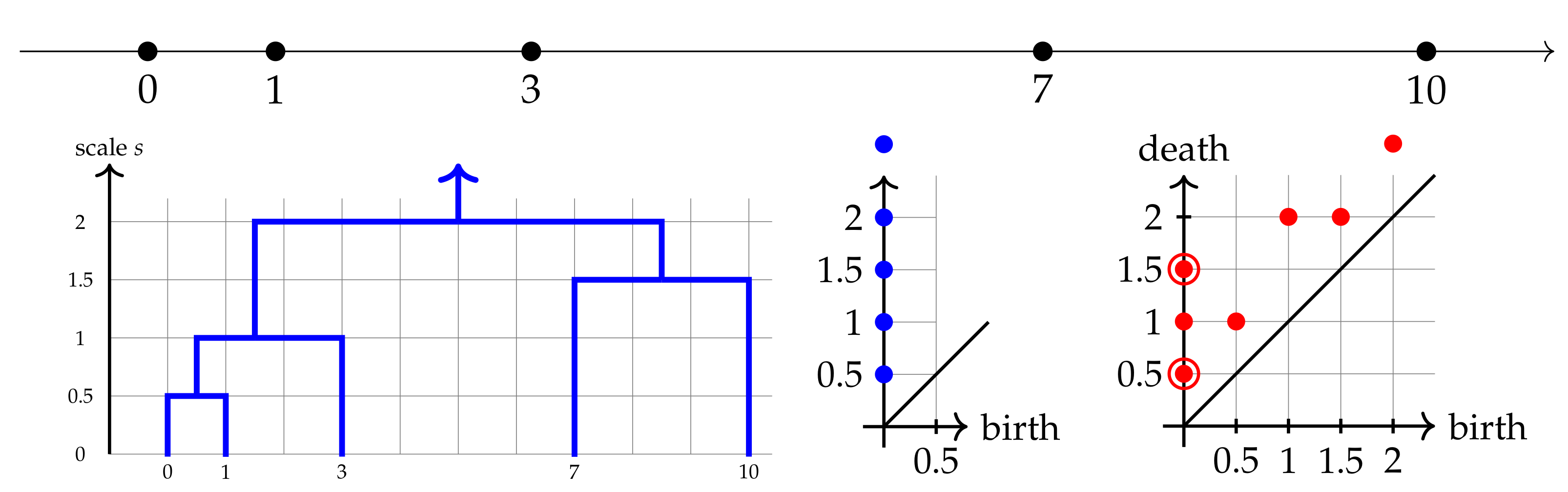
Figure 2 illustrates the key concepts before formal Definitions 1, 3 and 4 for the point cloud $A=\{0,1,3,7,10\}$ in the real line $\mathbb{R}$. Imagine that we gradually blur original data points by growing disks of the same radius s around the given points.

The disks of the closest points $0,1$ start overlapping at the scale $s=0.5$ when these points merge into one cluster $\{0,1\}$. This merger is shown by blue arcs joined at the node at $s=0.5$ in the single-linkage dendrogram; see the left picture at the bottom of Figure 2. The persistence diagram $\mathrm{PD}$ in the middle picture at the bottom of Figure 2 represents this merger by the pair $(0,0.5)$, meaning that a singleton cluster of (say) point 1 was born at the scale $s=0$ and then died later at $s=0.5$ by merging into another cluster of point 0.

When clusters $\{0,1,3\}$ and $\{7,10\}$ merge at $s=2$, this merger was earlier encoded in the persistence diagram by the single pair $(0,2)$, meaning that one cluster inherited from (say) point 7 was born at $s=0$ and died at $s=2$. The new mergegram in the bottom right picture of Figure 2 represents the above merger by the following two pairs. The pair $(1,2)$ means that the cluster $\{0,1,3\}$ is merging at the current scale $s=2$ and was previously formed at the smaller scale $s=1$. The pair $(1.5,2)$ means that another cluster $\{7,10\}$ is merging at the scale $s=2$ and was previously formed at $s=1.5$.

The 0D persistence diagram represents the cluster of the whole cloud A by the pair $(0,+\infty )$ because A was inherited from a singleton cluster starting from $s=0$. The mergegram represents the same cluster A by the pair $(2,+\infty )$ because A was formed during the last merger of $\{0,1,3\}$ and $\{7,10\}$ at $s=2$ and continues to live as $s\to +\infty$.

In the above dendrogram, every vertical arc going up from a scale b to d contributes one pair $(b,d)$ to the mergegram. So, both singleton clusters $\left\{7\right\}$, $\left\{10\right\}$ merging at $s=1.5$ contribute one pair $(0,1.5)$ of multiplicity two, shown by two red circles in Figure 2.

Definition 1

(single-linkage clustering). Let A be a finite set in a metric space X with a distance $d:X\times X\to [0,+\infty )$. For a distance threshold, which can be called a scale s, any points $a,b\in A$ should belong to oneSL clusterif and only if there is a finite sequence $a=a_1,\cdots ,a_m=b\in A$ such that any two successive points have a distance at most s, so $d(a_i,a_{i+1})\le s$ for $i=1,\cdots ,m-1$. Let ${\Delta }_{SL}(A;s)$ be the set of all single-linkage clusters at the scale s. For $s=0$, any point $a\in A$ forms a singleton cluster $\left\{a\right\}$. Representing each cluster from ${\Delta }_{SL}(A;s)$ over all $s\ge 0$ by one point gives thesingle-linkage dendrogram${\Delta }_{SL}\left(A\right)$ visualizing how clusters merge; see the first picture at the bottom of Figure 2.

For any $s>0$, all SL clusters ${\Delta }_{SL}(A;s)$ can be obtained as connected components of a Minimum Spanning Tree $\mathrm{MST}\left(A\right)$ by removing all edges longer than s.

Definition 2

(partition set $\mathbb{P}\left(A\right)$). For any set A, apartitionof A is a finite set of disjoint non-empty subsets $A_1,\cdots ,A_k\subset A$, whose union is A. The single set A forms thesingle-blockpartition of A. Thepartition set$\mathbb{P}\left(A\right)$ consists of all partitions of A.

The partition set $\mathbb{P}\left(A\right)$ of the abstract set $A=\{0,1,2\}$ consists of the five partitions

$$\left(\right\{0\},\{1\},\{2\left\}\right),\left(\right\{0,1\},\{2\left\}\right),\left(\right\{0,2\},\{1\left\}\right),\left(\right\{1,2\},\{0\left\}\right),\left(\right\{0,1,2\left\}\right).$$

For example, the collections $\left(\right\{0\},\{1\left\}\right)$ and $\left(\right\{0,1\},\{0,2\left\}\right)$ are not partitions of A.

Definition 3 below extends a dendrogram from (Reference [27], Section 3.1) to arbitrary (possibly, infinite) sets A. Every partition of A is finite by Definition 2. So, there is no need to add that an initial partition of A is finite. Hence, non-singleton sets are now allowed.

Definition 3

(dendrogram $\Delta$ of merge sets). A dendrogram Δ over any set A is a function $\Delta :[0,+\infty )\to \mathbb{P}\left(A\right)$ of a scale $s\ge 0$ satisfying the following conditions.

(a) There exists a scale $r\ge 0$ such that $\Delta (A;s)$ is the single block partition for $s\ge r$.

(b) If $s\le t$, then $\Delta (A;s)$ refines $\Delta (A;t)$, so any set from $\Delta \left(t\right)$ is a subset of some set from $\Delta (A;t)$. These inclusions of subsets of X induce the natural map ${\Delta }_s^t:\Delta \left(s\right)\to \Delta \left(t\right)$.

(c) There are finitely many merge scales $s_i$ such that

$$s_0=0and{s}_{i+1}=sup\{s\mid themap{\Delta }_s^{t}isidentityfor{s}^{\prime }\in [s_i,s)\},i=0,\cdots ,m-1.$$

Since $\Delta (A;s_i)\to \Delta (A;s_{i+1})$ is not an identity map, there is a subset $B\in \Delta \left(s_{i+1}\right)$, whose preimage consists of at least two subsets from $\Delta \left(s_i\right)$. This subset $B\subset X$ is a merge set with the birth scale $s_i$. All sets of $\Delta (A;0)$ are merge sets at the birth scale 0. The $\mathrm{life}\left(B\right)$ is the interval $[s_i,t)$ from its birth scale $s_i$ to its death scale $t=sup\{s\mid {\Delta }_{s_i}^s\left(B\right)=B\}$.

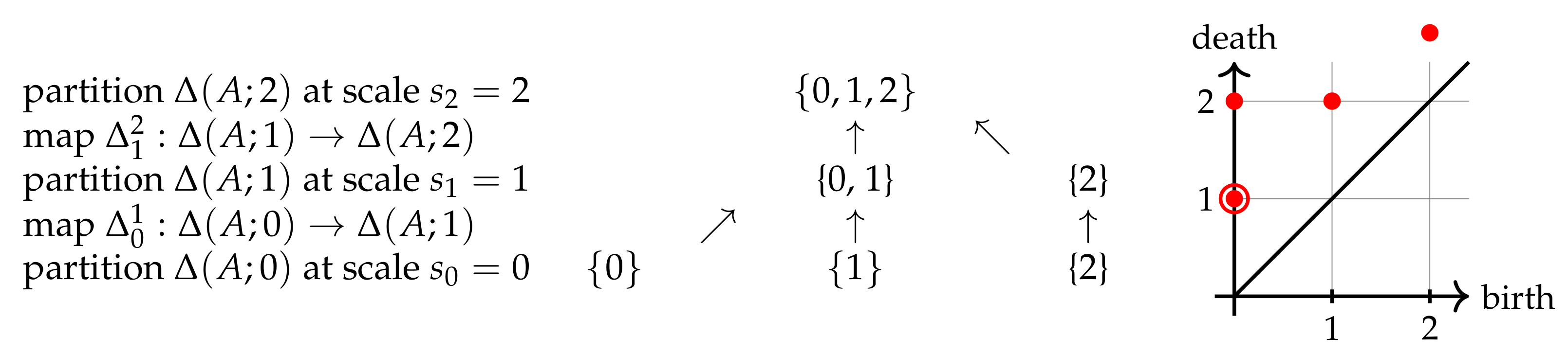
Dendrograms are often drawn as trees whose nodes represent all sets from the partitions $\Delta (A;s_i)$ at merge scales. Edges of such a tree connect any set $B\in \Delta (A;s_i)$ with its preimages under $\Delta (A;s_i)\to \Delta (A;s_{i+1})$. Figure 3 shows $\Delta$ for $A=\{0,1,2\}$.

In Figure 3, the partition $\Delta (A;1)$ consists of $\{0,1\}$ and $\left\{2\right\}$. The maps ${\Delta }_s^t$ induced by inclusions respect the compositions in the sense that ${\Delta }_s^t\circ {\Delta }_r^s={\Delta }_r^t$ for any $r\le s\le t$. For example, ${\Delta }_0^1\left(\left\{0\right\}\right)=\{0,1\}={\Delta }_0^1\left(\left\{1\right\}\right)$ and ${\Delta }_0^1\left(\left\{2\right\}\right)=\left\{2\right\}$, so ${\Delta }_0^1$ is a well-defined map from the partition $\Delta (A;0)$ of 3 singleton sets to $\Delta (A;1)$ but is not an identity.

At the scale $s_0=0$ the merge sets $\left\{0\right\},\left\{1\right\}$ have $\mathrm{life}=[0,1)$, the merge set $\left\{2\right\}$ has $\mathrm{life}=[0,2)$. At the scale $s_1=1$ the single merge set $\{0,1\}$ has $\mathrm{life}=[1,2)$. At the scale $s_2=2$ the single merge set $\{0,1,2\}$ has $\mathrm{life}=[2,+\infty )$. The first (Greek) letter in the word ‘dendrogram’ and a $\Delta$-shape of a typical tree motivate the notation $\Delta$.

Condition (Definition 3 (a)) says that a partition of a set X is trivial for all large scales. Condition (Definition 3 (b)) means that, if the scale s is increasing, any sets from a partition $\Delta \left(s\right)$ can merge but cannot split into smaller sets. Condition (Definition 3 (c)) implies that there are only finitely many mergers, when two or more subsets of X merge into a larger merge set.

Lemma 1

([7], Lemma 3.3). Given a metric space $(X,d)$ and a finite set $A\subset X$, the single-linkage dendrogram ${\Delta }_{SL}\left(X\right)$ from Definition 1 satisfies Definition 3.

A mergegram represents life spans of merge sets by pairs $(\mathrm{birth},\mathrm{death})\in {\mathbb{R}}^2$.

Definition 4

(mergegram $\mathrm{MG}(\Delta )$). The mergegram of a dendrogram Δ has the pair $(\mathrm{birth},\mathrm{death})\in {\mathbb{R}}^2$ for each merge set B of Δ with $\mathrm{life}\left(B\right)=[\mathrm{birth},\mathrm{death})$. If any life interval appears k times, the pair (birth,death) has the multiplicity k in $\mathrm{MG}(\Delta )$.

If our input is a point cloud A in a metric space, then the mergegram $\mathrm{MG}\left({\Delta }_{SL}\left(A\right)\right)$ is an isometry invariant of A because ${\Delta }_{SL}\left(A\right)$ depends only on inter-point distances. Though ${\Delta }_{SL}\left(A\right)$ as any dendrogram is unstable under perturbations of points, the key advantage of $\mathrm{MG}\left({\Delta }_{SL}\left(A\right)\right)$ is its stability, which will be proved in Theorem 4.

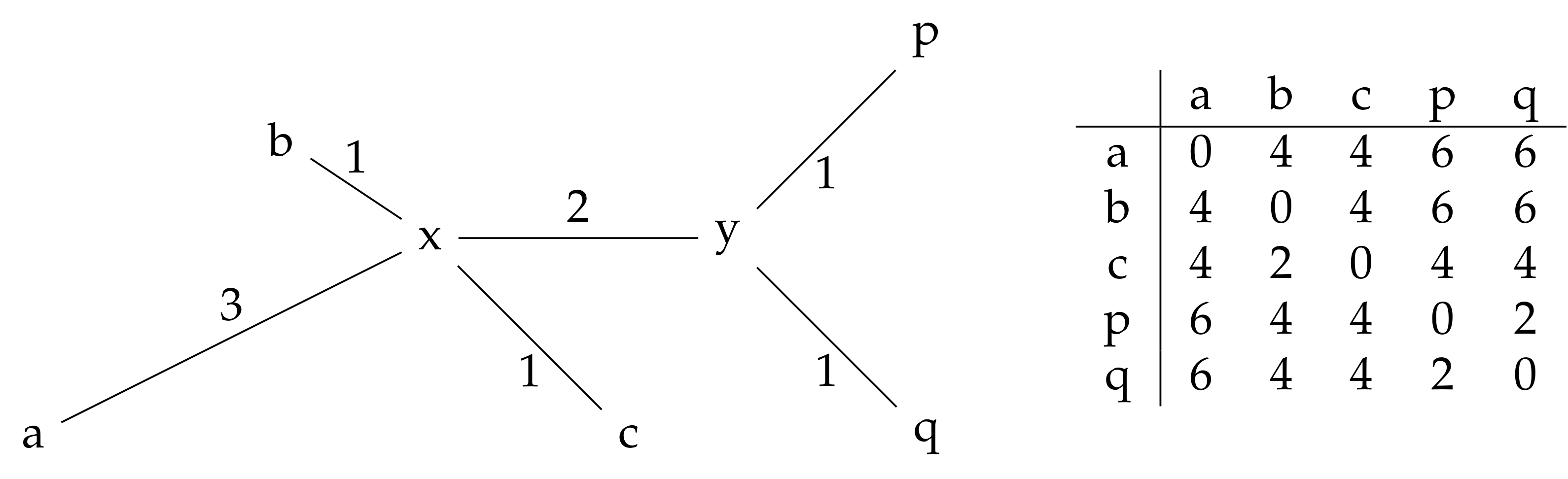
Figure 4 shows the metric space $X=\{a,b,c,p,q\}$ with distances defined by the shortest path metric induced by the specified edge-lengths; see the distance matrix.

The dendrogram $\Delta$ in the first picture of Figure 5 leads to the mergegram as follows:

• each of the 1-point sets $\left\{b\right\}$, $\left\{c\right\}$, $\left\{p\right\}$, $\left\{q\right\}$ has pair (0, 1), so its multiplicity is 4;
• each of the merge sets $\{b,c\}$ and $\{p,q\}$ has the pair (1,2), so its multiplicity is 2;
• the singleton set $\left\{a\right\}$ has the pair $(0,3)$; the merge set $\{b,c,p,q\}$ has the pair (2, 3);
• the full set $\{a,b,c,p,q\}$ continues to leave up to $s=3$, hence having the pair $(3,+\infty )$.

4. Explicit Relations between 0-Dimensional Persistence and Mergegram

This section recalls the concept of persistence and then shows how any 0D persistence and dendrogram in general position can be reconstructed from a mergegram.

Definition 5

(persistence module $\mathbb{V}$). A persistence module $\mathbb{V}$ over the real numbers $\mathbb{R}$ is a collection of vector spaces $V_t$, $t\in \mathbb{R}$ with linear maps $v_s^t:V_s\to V_t$, $s\le t$ such that $v_t^t$ is the identity on $V_t$, and the composition is respected: $v_s^t\circ v_r^s=v_r^t$ for any $r\le s\le t$.

The set of real numbers can be considered as a category $\mathbb{R}$ in the following sense. The objects of $\mathbb{R}$ are all real numbers. Any real numbers $a\le b$ define a single morphism $a\to b$. The composition of morphisms $a\to b$ and $b\to c$ is the morphism $a\le c$. In the language of category theory, a persistence module is a functor from $\mathbb{R}$ to the category of vector spaces. A basic example of a persistence module $\mathbb{V}$ is an interval module. An interval J between points $p<q$ in $\mathbb{R}$ can be one of the following types: closed $[p,q]$, open $(p,q)$, half-open or half-closed $[p,q)$ and $(p,q]$, all encoded as follows:

$$[p^{-},q^{+}]:=[p,q],[p^{+},q^{-}]:=(p,q),[p^{+},q^{+}]:=(p,q],[p^{-},q^{-}]:=[p,q).$$

The endpoints $p,q$ can have the infinite values $\pm \infty$, but without superscripts.

Example 2

(interval module $\mathbb{I}\left(J\right)$). Let $J\subset \mathbb{R}$ be an interval. The interval module $\mathbb{I}\left(J\right)$ is the persistence module defined by the following vector spaces $I_s$ and linear maps $i_s^t:I_s\to I_t$

$$I_s=\left\{\begin{array}{cc}{\mathbb{Z}}_2,\hfill & fors\in J,\hfill \\ 0,\hfill & otherwise;\hfill \end{array}\right.i_s^t=\left\{\begin{array}{cc}\mathrm{id},\hfill & fors,t\in J,\hfill \\ 0,\hfill & otherwise\hfill \end{array}\right.foranys\le t.$$

The direct sum $\mathbb{W}=\mathbb{U}\oplus \mathbb{V}$ of persistence modules $\mathbb{U},\mathbb{V}$ is defined as the persistence module with the vector spaces $W_s=U_s\oplus V_s$ and linear maps $w_s^t=u_s^t\oplus v_s^t$.

We illustrate the abstract concepts above by geometric constructions. Let $f:X\to \mathbb{R}$ be a continuous function on a topological space. The sublevel sets $X_s^f=f^{-1}\left((-\infty ,s]\right)$ form nested subspaces $X_s^f\subset X_t^f$ for any $s\le t$. The inclusions of the sublevel sets respect compositions similarly to a dendrogram $\Delta$ in Definition 3. On a metric space X with a metric $d:X\times X\to [0,+\infty )$, a typical example of a function $f:X\to \mathbb{R}$ is the distance $d_A$ to a finite subset $A\subset X$. For any point $p\in X$, let $d_A\left(p\right)$ be the distance from p to a closest point of A. For any $r\ge 0$, the preimage $X_r^{d_A}=d_A^{-1}\left((-\infty ,r]\right)=\{p\in X\mid d_A\left(p\right)\le r\}$ is the union of closed balls with radius r and centers at all points $q\in A$. For example, $X_0^{d_A}={d_A}^{-1}\left((-\infty ,0]\right)=A$ and $X_{+\infty }^{d_A}={d_A}^{-1}\left(\mathbb{R}\right)=X$.

Any continuous function $f:X\to \mathbb{R}$ induces the inclusion $X_s^f\subset X_r^f$ for any parameters $s\le r$. Then, all sublevel sets $X_s^f$ form a nested sequence of subspaces within X. The above construction of a filtration $\left\{X_s^f\right\}$ can be considered as a functor from $\mathbb{R}$ to the category of topological spaces. Below, we discuss the simplest case of dimension 0.

Example 3

(persistent homology). For any topological space X, the 0-dimensional homology $H_0\left(X\right)$ is the vector space (with coefficients ${\mathbb{Z}}_2$) generated by all connected components of X. Let $\left\{X_s\right\}$ be any filtration of nested spaces, e.g., sublevel sets $X_s^f$ based on a continuous function $f:X\to \mathbb{R}$. The inclusions $X_s\subset X_r$ for $s\le r$ induce the linear maps between homology groups $H_0\left(X_s\right)\to H_0\left(X_r\right)$ and define thepersistent homology$\left\{H_0\left(X_s\right)\right\}$, which satisfies the conditions of a persistence module from Definition 5.

If X is a finite set of m points, then $H_0\left(X\right)$ is the direct sum ${\mathbb{Z}}_2^m$ of m copies of ${\mathbb{Z}}_2$.

The persistence modules that are decomposable as direct sums of interval modules can be described in a simple combinatorial way by persistence diagrams in ${\mathbb{R}}^2$.

Definition 6

(persistence diagram $\mathrm{PD}\left(\mathbb{V}\right)$). Let a persistence module $\mathbb{V}$ be decomposed as a direct sum of interval modules : $\mathbb{V}\cong \underset{l\in L}{⨁}\mathbb{I}(p_l^{*},q_l^{*})$, where * is + or −. The persistence diagram $\mathrm{PD}\left(\mathbb{V}\right)$ is the multiset $\mathrm{PD}\left(\mathbb{V}\right)=\{(p_l,q_l)\mid l\in L\}\setminus \{p=q\}\subset {\mathbb{R}}^2$.

The 0-dimensional persistence diagram of a topological space X with a continuous function $f:X\to \mathbb{R}$ is denoted by $\mathrm{PD}\left\{H_0\left(X_s^f\right)\right\}$. Lemma 2 will prove that the merge module $M(\Delta )$ of any dendrogram $\Delta$ is decomposable into interval modules. The mergegram $\mathrm{MG}(\Delta )$ will be interpreted as the persistence diagram of $M(\Delta )$.

The following result describes how the persistence diagram $\mathrm{PD}$ of the distance-based filtration of any point cloud A can be obtained from the mergegram $\mathrm{MG}\left({\Delta }_{\mathrm{SL}}\left(S\right)\right)$.

Theorem 1

([7], Theorem 5.3). For any finite set A in a metric space $(X,d)$, let $d_A:X\to \mathbb{R}$ be the distance to A. Let the mergegram $\mathrm{MG}\left({\Delta }_{SL}\left(A\right)\right)$ be a multiset ${\left\{(b_i,d_i)\right\}}_{i=1}^k$, where some pairs can be repeated. Then, the persistence diagram $\mathrm{PD}\left\{H_0\left(X_s^{d_A}\right)\right\}$ is the difference of the multisets ${\left\{(0,d_i)\right\}}_{i=1}^k-{\left\{(0,b_i)\right\}}_{i=1}^k$ containing each pair $(0,s)$ exactly $\#b-\#d$ times, where $\#b$ is the number of births $b_i=s$, and $\#d$ is the number of deaths $d_i=s$. All trivial pairs $(0,0)$ are ignored, and, alternatively, we take ${\left\{(0,d_i)\right\}}_{i=1}^k$ only with $d_i>0$.

Theorem 1 is illustrated by Example 1, where $A=\{0,1,3,7,10\}$ has the diagram $\mathrm{PD}\left(A\right)=\left\{\right(0,0.5),(0,1),(0,1.5),(0,2),(0,+\infty \left)\right\}$ obtained from the mergegram

$$\mathrm{MG}\left({\Delta }_{\mathrm{SL}}\left(A\right)\right)=\{(0,0.5),(0,0.5),(0,1),(0,1.5),(0,1.5),(0.5,1),(1,2),(1.5,2),(2,+\infty )\}$$

as follows: one pair $(0,0.5)\in \mathrm{PD}\left(A\right)$ comes from two deaths and one birth $s=0.5$ in $\mathrm{MG}\left({\Delta }_{\mathrm{SL}}\left(A\right)\right)$. Similarly, each of the pairs $(0,1),(0,1.5),(0,2)\in \mathrm{PD}\left(A\right)$ comes from two deaths and one birth equal to the same scale s. The cloud $B=\{0,4,6,9,10\}\subset \mathbb{R}$ in Reference [7] (Example 1.1) has exactly the same $\mathrm{PD}\left(B\right)=\mathrm{PD}\left(A\right)$ but different $\mathrm{MG}\left({\Delta }_{\mathrm{SL}}\left(B\right)\right)\ne \mathrm{MG}\left({\Delta }_{\mathrm{SL}}\left(A\right)\right)$. This example jointly with Theorem 1 justify that the mergegram is strictly stronger than 0D persistence as an isometry invariant of a point cloud.

The New Reconstruction Theorem 2 below can be contrasted with the weakness of 0D persistence $\mathrm{PD}\left\{H_0\left(X_s^{d_A}\right)\right\}$ consisting of only pairs $(0,s)$ whose finite deaths are half-lengths of edges in a Minimum Spanning Tree $\mathrm{MST}\left(A\right)$. In Example 1, these scales $s=0.5,1,1.5,2$ are insufficient to reconstruct the SL dendrogram in Figure 2. Such a unique reconstruction is possible by using the richer invariant mergegram as follows.

Theorem 2

(from a mergegram to a dendrogram). Let A be a finite point cloud in general position in the sense that all merge scales of A in a dendrogram Δ from Definition 3 are different. Then, the dendrogram Δ can be reconstructed from its mergegram $\mathrm{MG}(\Delta )$, uniquely up to a permutation of nodes in Δ at scale $s=0$.

Proof. 

Consider all merge scales one by one in the increasing order starting from the smallest. The general position implies that only two clusters merge at any merge scale. For any current scale s, the mergegram contains exactly two pairs $(b_1,s)$ and $(b_2,s)$.

For a smallest merge scale $s>0$, the births should be $b_1=b_2=0$. We start drawing a dendrogram $\Delta$ by merging any two points of A at this smallest scale s. To realize a merger at any larger s, we should select two clusters representing $(b_1,s)$ and $(b_2,s)$.

If $b_i=0$, then we take any of the unmerged points of A. If $b_i>0$, then the already constructed dendrogram should contain a unique non-singleton cluster determined by the scale $b_i\in (0,s)$. Hence, at any merge scale s, we know how to select two clusters to merge. The only choice comes from choosing points of A or permuting notes of $\Delta$. □

Following the above proof of Theorem 2 for the cloud $A=\{0,1,3,7,10\}$ in Example 1, the first two pairs $(0,0.5)\in \mathrm{MG}\left({\Delta }_{\mathrm{SL}}\left(A\right)\right)$ indicate that we should merge two points of A at $s=0.5$. The scale $s=0.5$ uniquely determines this 2-point cluster.

The next two pairs $(0,1),(0.5,1)$ mean that the above cluster born at $s=0.5$ should merge at $s=1$ with a singleton cluster (any free point of A). The resulting 3-point cluster is uniquely determined by its merge scale $s=1$. The further two pairs $(0,1.5),(0,1.5)$ say that a new 2-point cluster is formed at $s=1.5$ by the two remaining points of A.

The final pairs $(1,2),(1.5,2)$ tell us to merge at $s=2$ the two clusters formed earlier at $s=1$ and $s=1.5$. The resulting dendrogram $\Delta$ has the expected combinatorial structure as in Figure 2, though we can draw $\Delta$ in another way by permuting points of A.

5. Stability of the Mergegram for Any Single-Linkage Dendrogram

This section fully proves the stability of a mergegram, which was stated in Reference [7] (Theorem 7.4), without proving key Lemmas 2 and 3. For simplicity, we consider vector spaces with coefficients only in ${\mathbb{Z}}_2=\{0,1\}$, which can be replaced by any field.

Definition 7 introduces homomorphisms between persistence modules, which are needed to state the stability of persistence diagrams $\mathrm{PD}\left\{H_0\left(X_s^f\right)\right\}$ under perturbations of a function $f:X\to \mathbb{R}$. This result will imply a stability for the mergegram $\mathrm{MG}\left({\Delta }_{SL}\left(A\right)\right)$ for the dendrogram ${\Delta }_{SL}\left(A\right)$ of the single-linkage clustering of a set $A\subset X$.

Definition 7

(a homomorphism between persistence modules). Let $\mathbb{U}$ and $\mathbb{V}$ be persistent modules over $\mathbb{R}$. A homomorphism $\mathbb{U}\to \mathbb{V}$ of a degree $\delta \in \mathbb{R}$ consists of linear maps ${\varphi }_t:U_t\to V_{t+\delta }$, $t\in \mathbb{R}$, such that the diagram below commutes for all $s\le t$.

Let ${\mathrm{Hom}}^{\delta }(\mathbb{U},\mathbb{V})$ be all homomorphisms $\mathbb{U}\to \mathbb{V}$ of degree δ. Persistence modules $\mathbb{U},\mathbb{V}$ areisomorphicif there are inverse homomorphisms $\mathbb{U}\to \mathbb{V}\to \mathbb{U}$ of degree 0.

For a persistence module $\mathbb{V}$ with maps $v_s^t:V_s\to V_t$, the simplest example of a homomorphism of a degree $\delta \ge 0$ is $1_{\mathbb{V}}^{\delta }:\mathbb{V}\to \mathbb{V}$ defined by the maps $v_s^{s+\delta }$, $t\in \mathbb{R}$. So, $v_s^t$ defining the structure of $\mathbb{V}$ shift all vector spaces $V_s$ by the difference $\delta =t-s$.

Interleaved modules defined below algebraically generalize a geometric perturbation of a set X in terms of (the homology of) its sublevel sets $X_s$.

Definition 8

(interleaving distance ID). Persistence modules $\mathbb{U}$ and $\mathbb{V}$ are called δ-interleaved if there are homomorphisms $\varphi \in {\mathrm{Hom}}^{\delta }(\mathbb{U},\mathbb{V})$ and $\psi \in {\mathrm{Hom}}^{\delta }(\mathbb{V},\mathbb{U})$ such that $\varphi \circ \psi =1_{\mathbb{V}}^{2\delta }\mathrm{and}\psi \circ \varphi =1_{\mathbb{U}}^{2\delta }$. The interleaving distance between the persistence modules $\mathbb{U}$ and $\mathbb{V}$ is $\mathrm{ID}(\mathbb{U},\mathbb{V})=inf\{\delta \ge 0\mid \mathbb{U}\mathrm{and}\mathbb{V}\mathrm{are}\delta -\mathrm{interleaved}\}.$

If $f,g:X\to \mathbb{R}$ are continuous functions such that $\left|\right|f-{g\left|\right|}_{\infty }\le \delta$ in the $L_{\infty }$-distance, the modules $H_k\left\{f^{-1}(-\infty ,s]\right\}$, $H_k\left\{g^{-1}(-\infty ,s]\right\}$ are $\delta$-interleaved for any k [15]. The last conclusion extends to persistence diagrams for the bottleneck distance below.

Definition 9

(bottleneck distance BD). Let $C,D$ be multisets of finitely many points $(p,q)\in {\mathbb{R}}^2$, $p<q$, of finite multiplicity and all diagonal points $(p,p)\in {\mathbb{R}}^2$ of infinite multiplicity. For $\delta \ge 0$, a δ-matching is a bijection $h:C\to D$ such that ${|h\left(a\right)-a|}_{\infty }\le \delta$ in the $L_{\infty }$-distance for any point $a\in C$. Thebottleneckdistance between modules $\mathbb{U},\mathbb{V}$ is defined as $\mathrm{BD}(\mathbb{U},\mathbb{V})=\inf \{\delta \mid \mathrm{there}\mathrm{is}\mathrm{a}\delta -\mathrm{matching}\mathrm{between}\mathrm{PD}(\mathbb{U}),\mathrm{PD}(\mathbb{V}\left)\right\}$.

Historically, stability of persistence for sequences of sublevel sets was extended as Theorem 3 to q-tame persistence modules. A persistence module $\mathbb{V}$ is q-tame if any non-diagonal square in the persistence diagram $\mathrm{PD}\left(\mathbb{V}\right)$ contains only finitely many of points; see Reference [16] (Section 2.8). Any finitely decomposable persistence module is q-tame.

Theorem 3

(stability of persistence modules [16], isometry Theorem 4.11). Let $\mathbb{U}$ and $\mathbb{V}$ be q-tame persistence modules. Then, $\mathrm{ID}(\mathbb{U},\mathbb{V})=\mathrm{BD}\left(\mathrm{PD}\right(\mathbb{U}),\mathrm{PD}(\mathbb{V}\left)\right)$, where $\mathrm{ID}$ is the interleaving distance, and $\mathrm{BD}$ is the bottleneck distance between persistence modules.

Definition 10

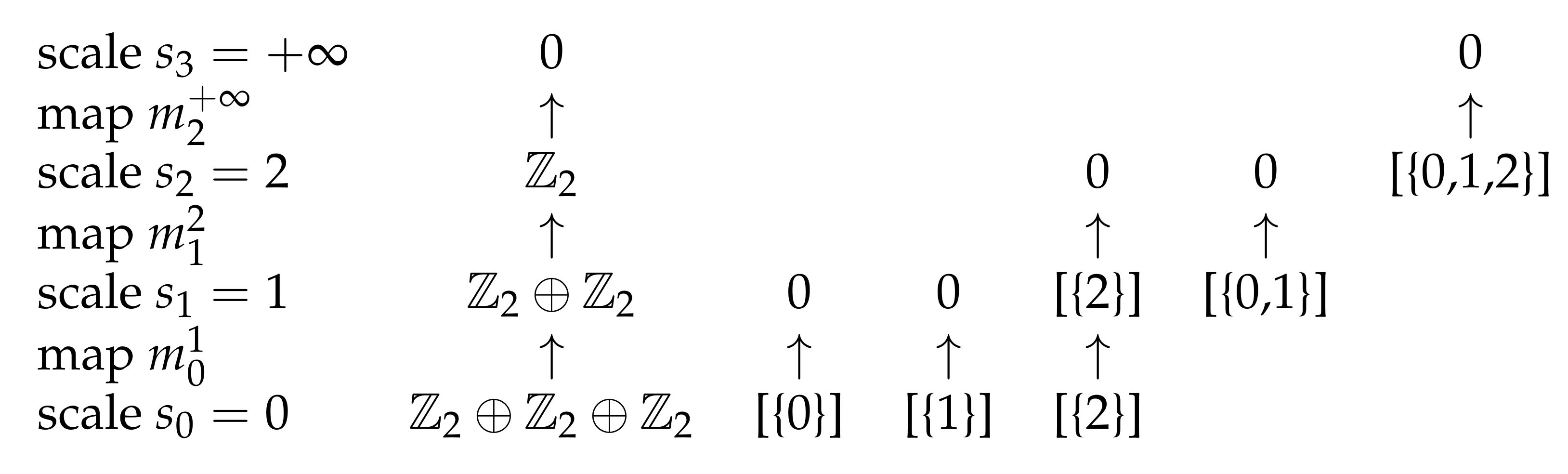
(merge module $M(\Delta )$). For any dendrogam Δ on a finite set X, the merge module $M(\Delta )$ consists of the vector spaces $M_s(\Delta )$, $s\in \mathbb{R}$, and linear maps $m_s^t:M_s(\Delta )\to M_t(\Delta )$, $s\le t$. For any $s\in \mathbb{R}$ and $A\in \Delta \left(s\right)$, the space $M_s(\Delta )$ has the generator or a basis vector $\left[A\right]\in M_s(\Delta )$. For $s<t$ and any set $A\in \Delta \left(s\right)$, if the image of A under ${\Delta }_s^t$ coincides with $A\subset X$, so ${\Delta }_s^t\left(A\right)=A$, then $m_s^t\left(\left[A\right]\right)=\left[A\right]$, else $m_s^t\left(\left[A\right]\right)=0$, see Figure 6.

In a dendrogram $\Delta$ from Definition 3, any merge set A of $\Delta$ has $\mathrm{life}\left(A\right)=[b,d)$ from its birth scale b to its death scale d. Lemmas 2 and 3 are proved for the first time.

Lemma 2

(merge module decomposition). For any dendrogram Δ from Definition 3, the merge module $M(\Delta )\cong \underset{A}{⨁}\mathbb{I}\left(\mathrm{life}\left(A\right)\right)$ decomposes over all merge sets A.

Proof 

(Proof of Lemma 2). The goal is to prove that $M(▵)\cong {⨁}_A\mathbb{I}\left(\mathrm{life}\left(A\right)\right)$. Recall that the interval module $\mathbb{I}\left(\mathrm{life}\right(A\left)\right)$ consists of only vector spaces 0 and ${\mathbb{Z}}_2$. For a scale r, let ${\mathbb{I}}_r\left(\mathrm{life}\left(A\right)\right)$ be its vector space, whose generator is denoted by $\left[{\mathbb{I}}_r\left(\mathrm{life}\left(A\right)\right)\right]$. Define

$${\psi }_r:M_r(▵)\to \underset{A}{⨁}{\mathbb{I}}_r\left(\mathrm{life}\left(A\right)\right)\mathrm{such}\mathrm{that}\left[A\right]\to \left[{\mathbb{I}}_r\left(\mathrm{life}\left(A\right)\right)\right]\mathrm{for}\mathrm{all}A\in ▵\left(r\right),$$

$${\varphi }_r:\underset{A}{⨁}{\mathbb{I}}_r\left(\mathrm{life}\left(A\right)\right)\to M_r(\Delta )\mathrm{such}\mathrm{that}\left[{\mathbb{I}}_r\left(\mathrm{life}\left(A\right)\right)\right]\to \left[A\right]\mathrm{for}\mathrm{all}\mathrm{life}\left(A\right)\mathrm{containing}r.$$

We will first prove that ${\varphi }_r$ is well-defined. If $r\in \mathrm{life}\left(A\right)$ then $A\in M_r(▵)$. We know that $M_r(▵)$ is generated by elements $A\in ▵\left(r\right)$ for which $r\in \mathrm{life}\left(A\right)$. Thus, the compositions satisfy ${\varphi }_r\circ {\psi }_r={\mathrm{id}}_r$ and ${\psi }_r\circ {\varphi }_r={\mathrm{id}}_r$. It remains to prove that morphisms correctly behave under the functors $\psi ,\varphi$. The proofs for both cases are essentially the same; thus, we will prove it only for $\psi$. The goal is to prove that the following diagram commutes:

Here, $i_s^t$ is the direct sum of the corresponding maps of interval modules ${⨁}_A{\left(i_s^t\right)}^A$ . Let $\left[A\right]$ be an arbitrary generator of $M_r(▵)$. There are two possibilities how $m_s^t$ can map $\left[A\right]$. If $t\in \mathrm{life}\left(A\right)$, then $m_s^t\left(\left[A\right]\right)=\left[A\right]\in M_t(▵)$ and by definition

$${\varphi }_t\circ m_s^t\left(\left[A\right]\right)=\left[{\mathbb{I}}_t\left(\mathrm{life}\left(A\right)\right)\right].$$

Since both $s,t\in \mathrm{life}\left(A\right)$, we also have that

$$m_s^t\circ {\varphi }_t\left(\left[A\right]\right)=\left[{\mathbb{I}}_t\left(\mathrm{life}\left(A\right)\right)\right]={\varphi }_t\circ m_s^t\left(\left[A\right]\right).$$

Assume now that $t\notin \mathrm{life}\left(A\right)$. Then, $m_s^t\left(\left[A\right]\right)=0$; thus, ${\varphi }_t\left(m_s^t\left(\left[A\right]\right)\right)=0$. On the other hand, $i_s^t\circ {\varphi }_s\left(\left[A\right]\right)=\left[{\mathbb{I}}_t\left(\mathrm{life}\left(A\right)\right)\right]={\mathbb{Z}}_2$. Since $t\notin \mathrm{life}\left(A\right)$, we get $i_s^t\circ {\varphi }_s\left(\left[A\right]\right)=0$. □

Lemma 3

(interleaving of merge modules). If subsets $A,B$ of a metric space $(X,d)$ have $\mathrm{HD}(A,B)=\delta$, then the merge modules $M\left({\Delta }_{SL}\left(A\right)\right)$, $M\left({\Delta }_{SL}\left(B\right)\right)$ are δ-interleaved.

Proof 

(Proof of Lemma 3). The equality $\mathrm{HD}(A,B)=\delta$ means that A is covered by the union of closed balls that have the radius $\delta$ and centers at all points $b\in B$. This union is the preimage is $d_B^{-1}\left([0,\delta ]\right)$, i.e., $A\subset d_B^{-1}\left([0,\delta ]\right)$. Extending the distance values by $s\ge 0$, we get $d_A^{-1}\left([0,s]\right)\subset d_B^{-1}\left([0,s+\delta ]\right)$ and similarly $d_B^{-1}\left([0,s]\right)\subset d_A^{-1}\left([0,s+\delta ]\right)$.

Let U be an arbitrary set in ${\Delta }_{SL}\left(A\right)$. Define map ${\varphi }_r:M(A;r)\to M(B;r+\delta )$

$${\varphi }_r\left(\left[U\right]\right)=\left\{\begin{array}{cc}\left[U\right],\hfill & \mathrm{if}r+\delta \in \mathrm{life}({\Delta }_{SL}\left(B\right),U),\hfill \\ 0,\hfill & \mathrm{otherwise}.\hfill \end{array}\right.$$

Symmetrically, for any $V\in {\Delta }_{SL}\left(B\right)$, we define ${\psi }_r:M(B;r)\to M(A;r+\delta )$

$${\psi }_r\left(\left[V\right]\right)=\left\{\begin{array}{cc}\left[V\right],\hfill & \mathrm{if}r+\delta \in \mathrm{life}({\Delta }_{SL}\left(A\right),V),\hfill \\ 0,\hfill & \mathrm{otherwise}.\hfill \end{array}\right.$$

In the notation above, $\mathrm{life}({\Delta }_{SL}\left(B\right),U)$ is the $\mathrm{life}\left(U\right)$ in the dendrogram ${\Delta }_{SL}\left(B\right)$. If $U\notin {\Delta }_{SL}\left(B\right)\left(t\right)$ for all values t, then $\mathrm{life}\left(U\right)=\varnothing$. By symmetry, it is enough to prove that the following diagrams commute:

We note first that, if $[a,b)=\mathrm{life}({\Delta }_{SL}\left(A\right),U)$, then $\mathrm{life}({\Delta }_{SL}\left(B\right),U)\subseteq [a-ϵ,b+ϵ)$.

We begin by proving commutativity of the first diagram. Let U be arbitrary element of ${\Delta }_{SL}\left(A\right)\left(s\right)$. If $t\notin \mathrm{life}({\Delta }_{SL}\left(A\right),U)$ then ${\varphi }_t\circ m_s^t=0$. If $s+\delta \notin \mathrm{life}({\Delta }_{SL}\left(B\right),U)$ or $t+\delta \notin \mathrm{life}({\Delta }_{SL}\left(B\right),U)$ then we are done. Since $t\notin \mathrm{life}({\Delta }_{SL}\left(A\right),U)$, it follows that $t+\delta \notin \mathrm{life}({\Delta }_{SL}\left(B\right),U)$. Thus, , with given assumptions, the diagram commutes.

Assume now that $t+\delta \notin \mathrm{life}({\Delta }_{SL}\left(A\right),U)$. Then, both ${\varphi }_t\left(m_s^t\left(U\right)\right)=0=m_{s+\delta }^{t+\delta }\left({\varphi }_s\left(U\right)\right)$. In the last case, we assume that $t\in \mathrm{life}({\Delta }_{SL}\left(A\right),U)$ and $t+\delta \in \mathrm{life}({\Delta }_{SL}\left(B\right),U)$. In this case, obviously, $s+\delta \in \mathrm{life}({\Delta }_{SL}\left(B\right),U)$; thus, ${\varphi }_t\left(m_s^t\left(\left[U\right]\right)\right)=\left[U\right]=m_{s+\delta }^{t+\delta }\left({\varphi }_s\left(\left[U\right]\right)\right)$.

For the second diagram, assume now that $U\in M\left({\Delta }_{SL}\left(A\right)\right)(s-\delta )$. Assume first that $s\notin \mathrm{life}({\Delta }_{SL}\left(B\right),U)$, then $s+\delta \notin \mathrm{life}({\Delta }_{SL}\left(B\right),U)$ and $m_{s-\delta }^{s+\delta }\left(\left[U\right]\right)=0={\psi }_s\left({\varphi }_{s-\delta }\left[U\right]\right)$.

Assume then that $s\in \mathrm{life}({\Delta }_{SL}\left(B\right),U)$. Now, the outcome of both maps ${\psi }_s$ and $m_{s-\delta }^{s+\delta }$ depends on whether $s+\delta \in \mathrm{life}({\Delta }_{SL}\left(A\right),U)$; thus, $m_{s-\delta }^{s+\delta }\left(\left[U\right]\right)={\psi }_s\left({\varphi }_{s-\delta }\left[U\right]\right)$. Since all the diagrams commute, the required conclusion follows. □

Theorem 4

(stability of a mergegram). The mergegrams of any finite point clouds $A,B$ in a metric space $(X,d)$ satisfy $\mathrm{BD}(\mathrm{MG}\left({\Delta }_{SL}\left(A\right)\right),\mathrm{MG}\left({\Delta }_{SL}\left(B\right)\right)\le \mathrm{HD}(A,B)$. Hence, any small perturbation of a cloud A in the Hausdorff distance leads to a similarly small perturbation in the bottleneck distance for its mergegram $\mathrm{MG}\left({\Delta }_{SL}\left(A\right)\right)$.

Proof. 

The given clouds $A,B\subset X$ with $\mathrm{HD}(A,B)=\delta$ have $\delta$-interleaved merge modules by Lemma 3, so $\mathrm{ID}(\mathrm{MG}\left({\Delta }_{SL}\left(A\right)\right),\mathrm{MG}\left({\Delta }_{SL}\left(B\right)\right)\le \delta$. Since any merge module $M(\Delta )$ is finitely decomposable, hence, it is q-tame by Lemma 2. The corresponding mergegram $\mathrm{MG}\left(M\right(\Delta \left)\right)$ satisfies Theorem 3, so $\mathrm{BD}(\mathrm{MG}\left({\Delta }_{SL}\left(A\right)\right),\mathrm{MG}\left({\Delta }_{SL}\left(B\right)\right)\le \delta$. □

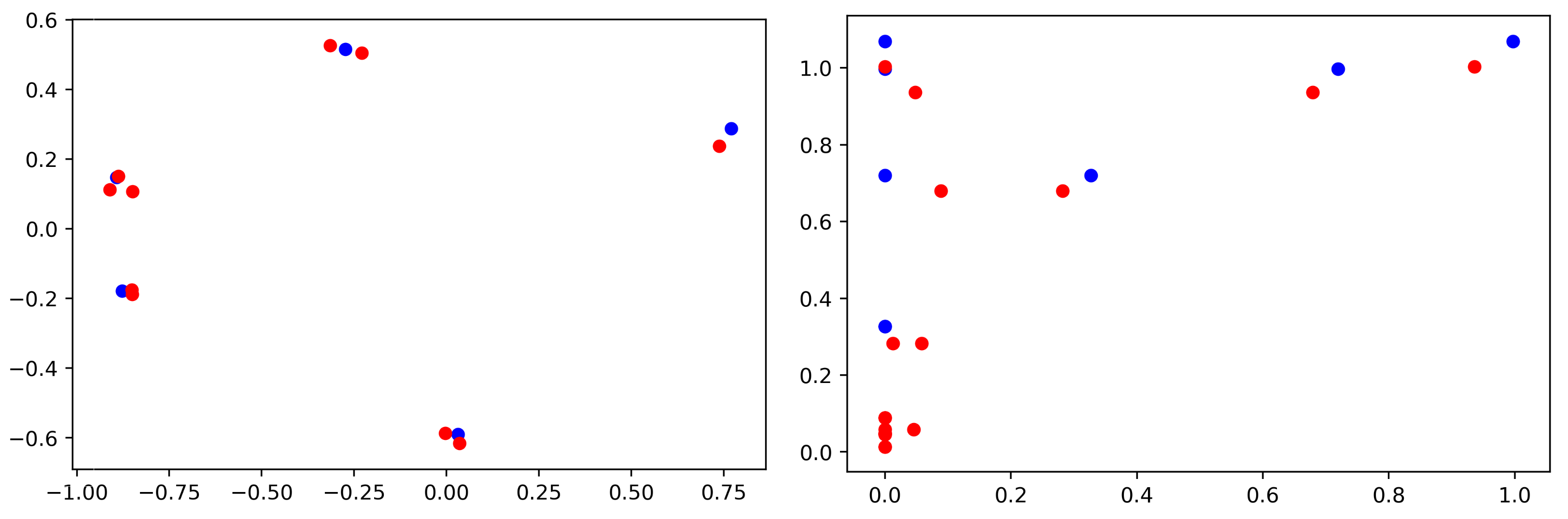
Figure 7 illustrates Theorem 4 on a cloud and its perturbation by showing their close mergegrams. The more extensive experiment on 100 clouds in Reference [7] (Figure 8) similarly confirms that the mergegram is perturbed within expected bounds. The computational complexity of the mergegram $\mathrm{MG}\left({\Delta }_{SL}\left(A\right)\right)$ was proved to be near linear in the number n of points in a cloud $A\subset {\mathbb{R}}^m$; see Reference [7] (Theorem 8.2). The results above justify that the invariant mergegram satisfies conditions (a,b,c) of Isometry Recognition Problem 1.

6. New Experiments on Isometry Recognition of Substantially Distorted Real Shapes

This section fulfills final condition (d) of Problem 1 by experimentally comparing the mergegram with 0D persistence and distributions of distances to neighbors on 15,000 clouds. The earlier paper by Reference [7] did experiments only on randomly generated clouds.

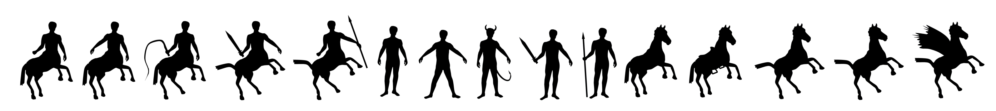
We considered 15 classes of shapes represented by black and white images of mythical creatures [9]; see Figure 1. These shapes were chosen to make the shape recognition problem really challenging. Indeed, similar creatures from this dataset are represented by slightly different shapes, which can be hard to isometrically distinguish from each other. For example, several images of a horse include only minor differentiating features, such as a saddle or a different tails, which makes horses nearly identical.

Shape generation. For each image, we generated 1000 perturbed images by affine and projective transformations to get 15,000 distorted shapes split into 15 classes.

First, we rotated each image around its central point by an angle generated uniformly in the interval $[0,2\pi )$ using the function cv::rotate from the OpenCV library. If needed, we extended the resulting image to fit all black pixels of the rotated shape into a bounding box. Then, both affine and projective transformations distort each image by using a noise parameter $\delta$ such that the value $\delta =0$ represents the identity transformation.

Figure 8 illustrates how an original image is randomly rotated, and then randomly distorted by affine or projective transformations, depending on the noise parameter $\delta$.

Affine transformations are implemented as compositions of the already applied rotations above and the function cv::resize() from the OpenCV library. This function scales an image of size $w\times h$ by horizontal and vertical factors $a,b$ sampled as follows.

• Uniform noise: $a\in [1-\delta w,1+\delta w]$, $b\in [1-\delta h,1+\delta h]$ have uniform distributions.
• Gaussian noise: $a\in \mathcal{N}(1,\delta h)\cap {\mathbb{R}}_{+}$ and $b\in \mathcal{N}(1,\delta w)\cap {\mathbb{R}}_{+}$ have Gaussian distributions with mean 1 and standard variance $\delta h,\delta v$, truncated to positive numbers.

Projective transformation are implemented as compositions of the already applied rotations above and the OpenCV function cv::getPerspectiveTransform() function, which is parametrized by 4-dimensional array $v=(a_0,a_1,a_2,a_3)$ consisting of points $a_i\in {\mathbb{Z}}^2$, $i=0,1,2,3$. This function maps the corners of the image as follows:

$$(0,0)\mapsto a_0,(0,h)\mapsto a_1,(w,0)\mapsto a_2\mathrm{and}(w,h)\mapsto a_3.$$

The projective transformation of the rectangle $w\times h$ is uniquely determined by the above corners. The above points $a_i$ are randomly sampled by using a noise parameter $\delta$.

• Uniform noise: each coordinate has a uniform distribution with a noise parameter $\delta$

  $$a_0\in [0,\delta w]\times [0,\delta h],a_1\in [0,\delta w]\times [h-\delta h,h],$$

  $$a_2\in [w-\delta w,w]\times [0,\delta h],a_3\in [w-\delta w,w]\times [h-\delta h,h].$$
• Gaussian noise: each coordinate has a Gaussian distribution truncated to the image

  $$a_0\in (\mathcal{N}(0,\delta w)\cap [0,w])\times (\mathcal{N}(0,\delta h)\cap [0,h]),$$

  $$a_1\in (\mathcal{N}(0,\delta w)\cap [0,w])\times (\mathcal{N}(h,\delta h)\cap [0,h]),$$

  $$a_2\in (\mathcal{N}(w,\delta w)\cap [0,w])\times (\mathcal{N}(0,\delta h)\cap [0,h]),$$

  $$a_3\in (\mathcal{N}(w,\delta w)\cap [0,w])\times (\mathcal{N}(h,\delta h)\cap [0,h]).$$

Point cloud extraction. For each distorted image, we extract classical Harris point corners [28] due to their simplicity; see the red points in Figure 8. For detecting corner points, the OpenCV function cv::cornerHarris was used with the parameters blockSize = 3, apertureSize = 5, k = 0.04, thresh = 120. However, one can use any reliable algorithms, such as FAST [29] or scale-invariant feature transform (SIFT) [30].

After describing the available point cloud data above, we specify condition (d) of Isometry Recognition Problem 1 in the context of supervised machine learning.

Problem 2

(experimental recognition). Given a labeled dataset split into classes of similar but projectively distorted shapes, develop a learning tool to recognize a class of distorted shapes with a highrecognition rate(percentage of correctly recognized classes).

Since all isometry invariants are independent of point ordering, the most suitable neural network is PersLay [20], whose output is invariant under permutations by design. Each layer is a combination of a coefficient layer $\omega \left(p\right):{\mathbb{R}}^m\to \mathbb{R}$, a transformation $\varphi \left(p\right):{\mathbb{R}}^m\to {\mathbb{R}}^q$ and a permutation invariant layer op combined as follows

$$\mathrm{PersLay}\left(D\right)=\mathrm{op}\left({\left\{w\left(p\right)\varphi \left(p\right)\right\}}_{p\in D}\right),\mathrm{where}D\mathrm{is}\mathrm{a}\mathrm{diagram}\mathrm{or}\mathrm{multiset}\mathrm{of}\mathrm{points}\mathrm{in}{\mathbb{R}}^m.$$

Coordinates of all input points are linearly normalized to $[0,1]$. We have used the following parameters of the PersLay network for all experiments below.

The max layer$\mathrm{MAX}\left(q\right)$ consists of the following functions.

• The coefficient layer $w:{\mathbb{R}}^m\to \mathbb{R}$ is the weight $w(x_1,\cdots ,x_m)=k|x_1-x_2|$, where k is a trainable scalar, and the dimension is typically $m=2$.
• The transformation layer $\varphi :\left\{\mathrm{diagrams}\mathrm{of}\mathrm{points}\mathrm{in}{\mathbb{R}}^m\right\}\to {\mathbb{R}}^q$ is the function $\varphi \left(D\right)={\sum }_{p\in D}\lambda p+\gamma \mathrm{maxpool}\left(D\right)+\beta$, where $\lambda$,$\gamma$ are ${\mathbb{R}}^{m\times q}$ trainable matrices, $\beta$ is a ${\mathbb{R}}^q$ trainable vector, and maxpool returns a maximum value for every $i=1,\cdots ,m$.
• The operational layer $\mathrm{op}:{\mathbb{R}}^q\to {\mathbb{R}}^t$ puts all coordinates in increasing order and composes the result with standard densely connected layer [31]$\mathrm{Dense}:{\mathbb{R}}^q\to {\mathbb{R}}^t$.

An output is a vector in ${\mathbb{R}}^t$ for $t=15$ of image classes. A final prediction is obtained by choosing a class with a largest coordinate in the output vector.

The image layer$\mathrm{Im}[x,y]$ for integer parameters $x,y$ and a multiset of points in the unit square ${[0,1]}^2$ consists of the following functions.

• The coefficient layer $w:{\mathbb{R}}^2\to \mathbb{R}$ is a piecewise constant function trained on $x·y$ parameters, defined on the unit square partition

  $$\mathcal{P}(x,y)=\left\{\left[\frac{i}{x},\frac{i+1}{x}\right]\times \left[\frac{j}{y},\frac{j+1}{y}\right]\mid i=0,\cdots ,x-1\mathrm{and}j=0,\cdots ,y-1\right\}.$$
• Let ${\varphi }_p:{\mathbb{R}}^2\to \mathbb{R}$ be the Gaussian distribution centered at $p\in D$ with a trainable standard deviation $\sigma$. The transformation layer $\varphi :\mathbb{R}\to {\mathbb{R}}^{xy}$ consists of $xy$ functions ${\varphi }_p$, where p runs over all centroids of the partition $\mathcal{P}(x,y)$.
• The operation layer op takes the sum over the given point cloud. A final prediction is made by composing the operation layer with the Dense layer.

Finally, the PersLay network used the optimizer tf.keras.adam with the standard learning rate 0.01 and 150 epochs, the loss function SparseCategoricalCrossEntropy, the 80:20 of training and testing, a 5-fold Monte Carlo cross validation for each run.

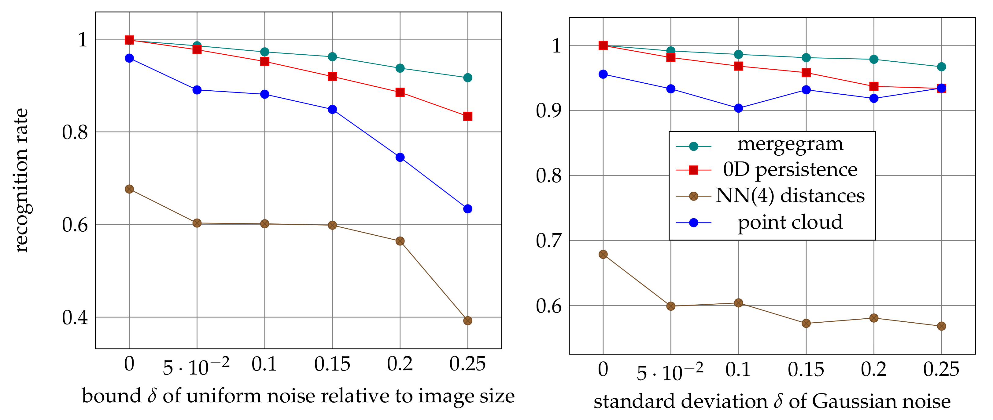
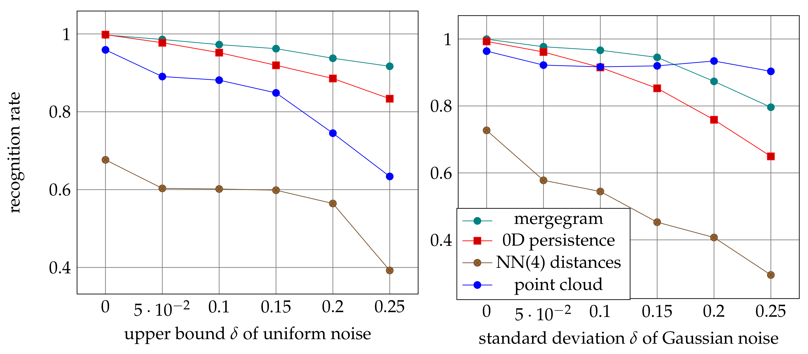
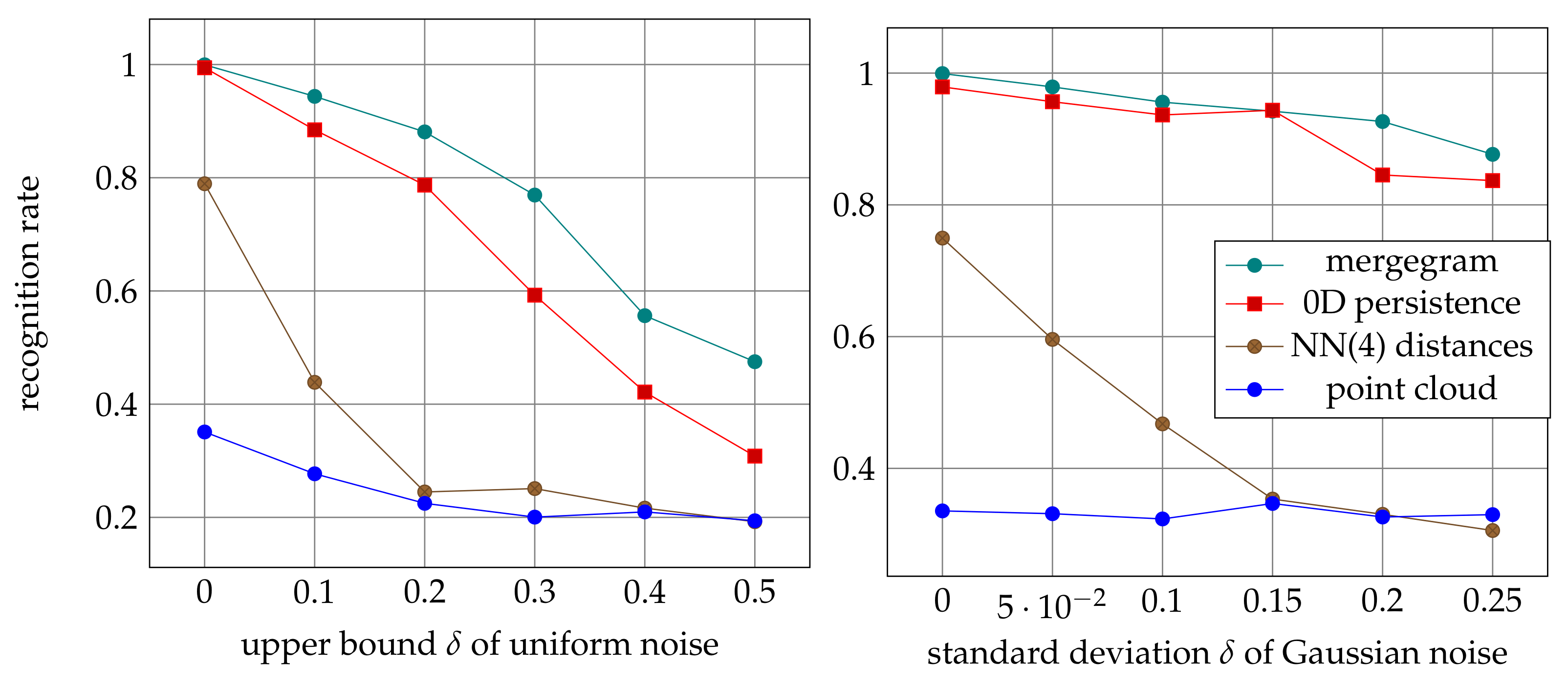
Figure 9, Figure 10 and Figure 11 show that the mergegram $\mathrm{MG}$ consistently outperforms two other isometry invariants: 0D persistence and the multiset $NN\left(4\right)$ consisting of 4-tuple distances to neighbors per given point. The simpler multiset $NN\left(2\right)$ performed worse. A given cloud $C\subset {\mathbb{R}}^2$ was considered as a baseline input. The noise factors $\delta$ reached 25%, which means that original images were distorted up to a quarter of image sizes.

7. A Discussion of Novel Contributions and Further Open Problems

This paper has further demonstrated that the provably stable-under-noise invariant mergegram of a dendrogram is a fast and efficient tool in the challenging problem of isometry shape recognition, especially for substantially distorted images.

In comparison with the conference version [7], Section 4 proved new Theorem 2 describing how to reconstruct a single-linkage dendrogram in general position from its much simpler mergegram. It is hard to define a continuous metric between dendrograms, especially because they can be unstable under perturbations. Theorem 2 allows us to measure a continuous similarity between dendrograms in general position as the bottleneck distance between their unique mergegrams. This distance can be computed in time $O(n^{1.5}logn)$[32] for diagrams consisting of at most n points.

Section 5 provided a full proof of stability of the mergegram under perturbations of points, while the earlier paper by Reference [7] only announced this result without proving highly non-trivial Lemmas 2 and 3, which required a heavy algebraic machinery.

In addition to Example 1 and Theorem 1 showing that the mergegram is stronger than 0D persistence, its strength is confirmed by the new experiments on 15,000 point samples from substantially distorted real shapes. In Figure 9, Figure 10 and Figure 11, the mergegram outperformed other isometry invariants. Since the distribution $NN\left(2\right)$ of distances to two closest neighbors per point performed badly, we have tried distances to four nearest neighbors, but this $NN\left(4\right)$ performed worse than the original cloud because of noise.

For very high levels of 20% and 25% distortions in projective transformations, the PersLay network trained on a point cloud achieved high recognition rates because we have extensively tried many parameters in the layers MAX(75) and Im[20,20] for a best trade-off between accuracy and speed. The C++ code for the mergegram is at Reference [7].

The recent stronger invariants are Pointwise Distance Distributions [33]. Their generic completeness under isometry holds in a more challenging setting of periodic point sets [34,35,36,37,38].

References

- Pauly, M.; Gross, M.; Kobbelt, L.P. Efficient simplification of point-sampled surfaces. In Proceedings of the IEEE Visualization, Boston, MA, USA, 27 October–1 November 2002; pp. 163–170. [Google Scholar]
- Zwicker, M.; Pauly, M.; Knoll, O.; Gross, M. Pointshop 3D: An interactive system for point-based surface editing. ACM Trans. Graph. (TOG) 2002, 21, 322–329. [Google Scholar] [CrossRef] [Green Version]
- Boutin, M.; Kemper, G. On reconstructing n-point configurations from the distribution of distances or areas. Adv. Appl. Math. 2004, 32, 709–735. [Google Scholar] [CrossRef] [Green Version]
- Huttenlocher, D.P.; Klanderman, G.A.; Rucklidge, W.J. Comparing images using the Hausdorff distance. Trans. Pattern Anal. Mach. Intell. 1993, 15, 850–863. [Google Scholar] [CrossRef] [Green Version]
- Chew, P.; Goodrich, M.; Huttenlocher, D.; Kedem, K.; Kleinberg, J.; Kravets, D. Geometric pattern matching under Euclidean motion. Comput. Geom. 1997, 7, 113–124. [Google Scholar] [CrossRef] [Green Version]
- Goodrich, M.T.; Mitchell, J.S.; Orletsky, M.W. Approximate geometric pattern matching under rigid motions. Trans. Pattern Anal. Mach. Intell. 1999, 21, 371–379. [Google Scholar] [CrossRef] [Green Version]
- Elkin, Y.; Kurlin, V. The mergegram of a dendrogram and its stability. In Proceedings of the MFCS 2020, Prague, Czech Republic, 24–28 August 2020. [Google Scholar]
- Bronstein, A.M.; Bronstein, M.M.; Kimmel, R. Numerical Geometry of Non-Rigid Shapes; Springer: Berlin/Heidelberg, Germany, 2008. [Google Scholar]
- Bronstein, A.M.; Bronstein, M.M.; Bruckstein, A.M.; Kimmel, R. Analysis of two-dimensional non-rigid shapes. Int. J. Comput. Vis. 2008, 78, 67–88. [Google Scholar] [CrossRef] [Green Version]
- Elad, A.; Kimmel, R. Bending invariant representations for surfaces. In Proceedings of the Computer Vision and Pattern Recognition, Kauai, HI, USA, 8–14 December 2001. [Google Scholar]
- Ovsjanikov, M.; Mérigot, Q.; Mémoli, F.; Guibas, L. One point isometric matching with the heat kernel. In Computer Graphics Forum; Blackwell Publishing: Oxford, UK, 2010; Volume 29, pp. 1555–1564. [Google Scholar]
- Ovsjanikov, M.; Bronstein, A.M.; Bronstein, M.M.; Guibas, L.J. Shape google: A computer vision approach to isometry invariant shape retrieval. In Proceedings of the ICCV Workshops, Kyoto, Japan, 27 September–4 October 2009; pp. 320–327. [Google Scholar]
- Mémoli, F.; Sapiro, G. A theoretical and computational framework for isometry invariant recognition of point cloud data. Found. Comput. Math. 2005, 5, 313–347. [Google Scholar] [CrossRef] [Green Version]
- Verri, A.; Uras, C.; Frosini, P.; Ferri, M. On the use of size functions for shape analysis. Biol. Cybern. 1993, 70, 99–107. [Google Scholar] [CrossRef]
- Cohen-Steiner, D.; Edelsbrunner, H.; Harer, J. Stability of persistence diagrams. Discret. Comput. Geom. 2007, 37, 103–120. [Google Scholar] [CrossRef] [Green Version]
- Chazal, F.; De Silva, V.; Glisse, M.; Oudot, S. The Structure and Stability of Persistence Modules; Springer: Berlin/Heidelberg, Germany, 2016. [Google Scholar]
- Parsa, S. A Deterministic O(m log m) Time Algorithm for the Reeb Graph. Discret. Comput. Geom. 2013, 49, 864–878. [Google Scholar] [CrossRef]
- Morozov, D.; Beketayev, K.; Weber, G. Interleaving distance between merge trees. Discret. Comput. Geom. 2013, 49, 52. [Google Scholar]
- Smith, P.; Kurlin, V. Skeletonisation algorithms with theoretical guarantees for unorganised point clouds with high levels of noise. Pattern Recognit. 2021, 115, 107902. [Google Scholar] [CrossRef]
- Carriere, M.; Chazal, F.; Ike, Y.; Lacombe, T.; Royer, M.; Umeda, Y. PersLay: A Neural Network Layer for Persistence Diagrams and Graph Topological Signatures. In Proceedings of the 23rd International Conference on Artificial Intelligence and Statistics (AISTATS), Palermo, Italy, 26–28 August 2020. [Google Scholar]
- Zaheer, M.; Kottur, S.; Ravanbakhsh, S.; Poczos, B.; Salakhutdinov, R.R.; Smola, A.J. Deep sets. In Proceedings of the Advances in Neural Information Processing Systems, Long Beach, CA, USA, 4–9 December 2017; pp. 3391–3401. [Google Scholar]
- Fu, G.; Hou, C.; Yao, X. Learning topological representation for networks via hierarchical sampling. In Proceedings of the International Joint Conference on Neural Networks (IJCNN), Budapest, Hungary, 14–19 July 2019; pp. 1–8. [Google Scholar]
- Cirrincione, G.; Ciravegna, G.; Barbiero, P.; Randazzo, V.; Pasero, E. The GH-EXIN neural network for hierarchical clustering. Neural Netw. 2020, 121, 57–73. [Google Scholar] [CrossRef] [PubMed]
- Karim, M.R.; Beyan, O.; Zappa, A.; Costa, I.G.; Rebholz-Schuhmann, D.; Cochez, M.; Decker, S. Deep learning-based clustering approaches for bioinformatics. Briefings Bioinform. 2021, 22, 393–415. [Google Scholar] [CrossRef] [PubMed] [Green Version]
- Clough, J.; Byrne, N.; Oksuz, I.; Zimmer, V.A.; Schnabel, J.A.; King, A. A topological loss function for deep-learning based image segmentation. Trans. PAMI 2020. [Google Scholar] [CrossRef]
- Gabrielsson, R.B.; Nelson, B.J.; Dwaraknath, A.; Skraba, P. A topology layer for machine learning. In Proceedings of the International Conference Artificial Intelligence and Statistics, Virtually, 26–28 August 2020; pp. 1553–1563. [Google Scholar]
- Carlsson, G.; Memoli, F. Characterization, stability and convergence of hierarchical clustering methods. J. Mach. Learn. Res. 2010, 11, 1425–1470. [Google Scholar]
- Sánchez, J.; Monzón, N.; Salgado De La Nuez, A. An analysis and implementation of the harris corner detector. Image Process. Line 2018, 8, 305–328. [Google Scholar] [CrossRef]
- Rosten, E.; Porter, R.; Drummond, T. Faster and better: A machine learning approach to corner detection. IEEE Trans. Pattern Anal. Mach. Intell. 2008, 32, 105–119. [Google Scholar] [CrossRef] [PubMed] [Green Version]
- Lowe, D.G. Object recognition from local scale-invariant features. In Proceedings of the Seventh IEEE International Conference on Computer Vision, Kerkyra, Greece, 20–27 September 1999; Volume 2, pp. 1150–1157. [Google Scholar]
- Abadi, M.; Agarwal, A.; Barham, P.; Brevdo, E.; Chen, Z.; Citro, C.; Corrado, G.S.; Davis, A.; Dean, J.; Devin, M.; et al. Tensorflow: Large-scale machine learning on heterogeneous distributed systems. arXiv 2016, arXiv:1603.04467. [Google Scholar]
- Kerber, M.; Morozov, D.; Nigmetov, A. Geometry Helps to Compare Persistence Diagrams. In Proceedings of the ALENEX, Arlington, VA, USA, 10–13 January 2016; pp. 103–112. [Google Scholar]
- Widdowson, D.; Kurlin, V. Pointwise distance distributions of periodic sets. arXiv 2021, arXiv:2108.04798. [Google Scholar]
- Mosca, M.; Kurlin, V. Voronoi-Based Similarity Distances between Arbitrary Crystal Lattices. Cryst. Res. Technol. 2020, 55, 1900197. [Google Scholar] [CrossRef]
- Anosova, O.; Kurlin, V. Introduction to Periodic Geometry and Topology. arXiv 2021, arXiv:2103.02749. [Google Scholar]
- Anosova, O.; Kurlin, V. An isometry classification of periodic point sets. In Proceedings of the Discrete Geometry and Mathematical Morphology, Uppsala, Sweden, 24–27 May 2021. [Google Scholar]
- Edelsbrunner, H.; Heiss, T.; Kurlin, V.; Smith, P.; Wintraecken, M. The Density Fingerprint of a Periodic Point Set. In Proceedings of the SoCG, Virtually, 7–10 June 2021. [Google Scholar]
- Widdowson, D.; Mosca, M.; Pulido, A.; Kurlin, V.; Cooper, A. Average Minimum Distances of Periodic Point Sets. MATCH Communications in Mathematical and in Computer Chemistry. Available online: https://match.pmf.kg.ac.rs (accessed on 6 July 2021).
Figure 1.
Images from the dataset of mythical creatures at http://tosca.cs.technion.ac.il (accessed on 25 August 2021) [8,9].
Figure 2.
Top: the 5-point cloud . Bottom: from left to right: single-linkage dendrogram from Definition 1, the 0D persistence diagram in Definition 6, the novel mergegram from Definition 4, where double circles show pairs of multiplicity 2.
Figure 3.
The dendrogram on and its mergegram from Definition 4.
Figure 4.
The set has the distance matrix obtained by the shortest path metric.
Figure 5.
Left: the dendrogram for the single linkage clustering of the set 5-point set in Figure 4. Right: the mergegram with one pair (0,1) of multiplicity 4.
Figure 6.
The merge module of the dendrogram on the set in Figure 3.
Figure 7.
Left: the cloud C of 5 blue points is close to the cloud of 10 red points in the Hausdorff distance. Right: the mergegrams are close in the bottleneck distance as predicted by Theorem 4.
Figure 8.
Generating distorted shapes by applying random rotations, affine and projective transformations, which substantially affect the extracted clouds of Harris corner points [28] in red.
Figure 9.
Recognition rates are obtained by training the max layer MAX(75) of PersLay on three isometry invariants and a cloud of corner points extracted from 15,000 affinely distorted images.
Figure 10.
Recognition rates are obtained by training the max layer MAX(75) of PersLay on isometry invariants and corner points extracted from 15,000 projectively distorted images.
Figure 11.
Recognition rates are obtained by training the image layer IM[20,20] of PersLay on isometry invariants and a cloud of corner points extracted from 15,000 affinely distorted images.
Publisher’s Note: MDPI stays neutral with regard to jurisdictional claims in published maps and institutional affiliations. |
© 2021 by the authors. Licensee MDPI, Basel, Switzerland. This article is an open access article distributed under the terms and conditions of the Creative Commons Attribution (CC BY) license (https://creativecommons.org/licenses/by/4.0/).
Share and Cite
MDPI and ACS Style
Elkin, Y.; Kurlin, V. Isometry Invariant Shape Recognition of Projectively Perturbed Point Clouds by the Mergegram Extending 0D Persistence. Mathematics 2021, 9, 2121. https://doi.org/10.3390/math9172121
AMA Style
Elkin Y, Kurlin V. Isometry Invariant Shape Recognition of Projectively Perturbed Point Clouds by the Mergegram Extending 0D Persistence. Mathematics. 2021; 9(17):2121. https://doi.org/10.3390/math9172121
Chicago/Turabian StyleElkin, Yury, and Vitaliy Kurlin. 2021. "Isometry Invariant Shape Recognition of Projectively Perturbed Point Clouds by the Mergegram Extending 0D Persistence" Mathematics 9, no. 17: 2121. https://doi.org/10.3390/math9172121
Note that from the first issue of 2016, this journal uses article numbers instead of page numbers. See further details here.