1. Introduction
Network analysis is becoming a powerful tool for describing the complex systems that arise in physical, biomedical, epidemiological, and social sciences, see in [
1,
2]. In particular, estimating network structure and its complexity from high-dimensional data has been one of the most relevant statistical challenges of the last decade [
3]. The mathematical framework to use depends on the type of relationship among the variables that the network should incorporate. For example, in the context of gene regulatory networks (GRN), traditional co-expression methods are useful to capture marginal correlation among genes without distinguishing between direct or mediated gene interactions. Instead, graphical models (GM) constitute a well-known framework for describing conditional dependency relationships between random variables in a complex system. Therefore, they are more suited to describe direct relations among genes, not mediated by the remaining genes.
In the GMs’ framework, an undirected graph describes the joint distribution of the random vector , the individual variables being the graph’s nodes and the edges reflecting the presence/absence of conditional dependency relation among them. When the system of random variables has a multivariate Gaussian distribution , we refer to Gaussian Graphical Models (GGMs). In such a case, the graph estimation is equivalent to estimating the precision matrix’s support, namely, the inverse of the covariance matrix associated with the multivariate Gaussian distribution.
There is extensive literature on learning a GGM, and we refer to the works in [
4,
5,
6,
7] for an overview. In brief, under high-dimensional setting and sparsity assumptions on the precision matrix, we can broadly classify the available methods into two categories: methods that estimate the entire precision matrix
and those that estimate only its support (i.e., the edge set
E). Methods in the first category usually impose a Lasso type penalty on the inverse covariance matrix entries when maximizing the log-likelihood, as the GLasso approach proposed in [
8,
9]. Methods in the second category date back to the seminal paper of Meinshausen and Bühlmann [
10] and use the variable selection properties of Lasso regression.
In recent years, the focus shifted from the inference of a single graph given a dataset to the inference of multiple graphs given different datasets, assuming that the graphs share some common structure. This setting encompasses cases where datasets measure similar entities (variables) under different conditions or setups. It is useful for describing various situations encountered in real applications, such as meta-analyses and heterogeneous data integration. For example, in GNR, a single dataset might represent the gene expression levels of
n patients affected by a particular type of cancer, and the inference aims to understand the specific regulatory mechanisms. International projects, such as The Cancer Genome Atlas (TGCA), or large repositories, such as Gene Expression Omnibus (GEO), make available tens of thousands of gene expression samples. Therefore, it is easy to find several datasets (i.e., different studies collected using different high-throughput assays or performed in different laboratories) on the experimental condition of interest. Assuming that, despite the difference in the technologies and preprocessing, the hidden regulatory mechanisms investigated in the different studies are similar if not the same, it is worth integrating them to improve the inference. A similar type of challenge is also present in the integrative multi-omics analysis. For instance, one can measure gene expression, single nucleotide polymorphisms (SNPs), methylation levels, etc. on the same set of individuals and want to combine the information across the different omics. In both cases, it is possible to develop multitasking or joint learning approaches to gain power in the inference (see [
11,
12] to cite few examples).
More specifically, in multiple GGMs inference, we have different datasets , each drawn from a Gaussian distribution . Each dataset measures (almost) the same sets of variables in a specific class (or condition) k. The aim is to estimate the underlying GGMs under the assumption that they share some common structure across the classes.
Several methods are already available in the literature to deal with such a problem. They differ on the assumptions on how the conditional dependency structure is shared across the various distributions. The majority of these methods extend maximum likelihood (MLE) approaches to the multiple data framework. Among the most important contributions, we cite the work in [
13] that penalizes the MLE by a hierarchical penalty enforcing similar sparsity patterns across classes, allowing some class-specific difference. However, as the penalty is not convex, convergence is not guaranteed. JGL [
14] is another important method that proposes two alternatives. The first penalizes the MLE by a fused Lasso penalty, and the second penalizes the MLE by combining two group Lasso penalties. In this last alternative, the two penalties enforce a similar sparsity structure and some differences, respectively. Two other approaches are [
15], which penalizes the MLE by an adaptive Lasso penalty whose weights are updated iteratively, and the work in [
16], which penalizes the MLE by a group Lasso penalty. On the other hand, the work in [
17,
18] extends the regression-based approach in [
10] to the multiple data setting. In particular, in [
17], the authors constructed a two-step procedure. In the first step, they infer the graphical structure using a regression-based approach with a group Lasso penalty for exploiting the common structure across the classes. In the second step, they penalize the MLE subject to the first step edges’ set. The authors of [
18] proposed regression-based minimization problem with cooperative group Lasso penalty. The first term is the standard group Lasso penalty which enforces the same structure across classes by penalizing elements of precision matrices. The second one penalizes negative elements of those matrices to promote differences between classes. By authors’ hypothesis, swap in the sign can occur only for class-specific connections, justifying such penalty.
In this paper, we propose
jewel, a new technique for jointly estimate a GGM in the multiple dataset framework. We assume that the underlying graph structure is the same across the
K classes. However, each class preserves its specific precision matrix. We extend the regression-based method proposed in [
10] to the case of multiple datasets, in the same spirit as in [
18] and the first step of the procedure in [
17], which mainly differ in the definition of variables’ groups. More specifically, in [
17,
18] the groups are determined by the
positions across the
K precision matrices and in our approach, the groups are determined by both
and
positions across the
K precision matrices. Consequently, both [
17,
18] do not provide symmetric estimates of precision matrices’ supports and require postprocessing. Instead,
jewel grouping strategy exploits both the common structure across the datasets and the symmetry of the precision matrices support. We consider this a valuable improvement compared to the competitors as such an approach allows to avoid the need for postprocessing.
The rest of the paper is organized as follows. In
Section 2, we derive the
jewel method and present the numerical algorithm for its solution, as well as establish the theoretical properties of the estimator in
Section 2.4 and discuss the choice of the tuning parameter in
Section 2.5. Code is provided in
Section 2.6. Finally, in
Section 3, we illustrate our method’s performance in a simulation study comparing it with some other available alternatives and describe a real data application from gene expression datasets.
2. Jewel: Joint Node-Wise Estimation of Multiple Gaussian Graphical Models
This section describes the mathematical setup, the proposed method for the joint estimation of GGMs (jewel), the numerical algorithm adopted, the theoretical property of the proposed estimator and approaches of estimating the regularization parameter.
2.1. Problem Setup
Let be datasets of dimension , respectively, that represent similar entities measured under K different conditions or collected in distinct classes. Each dataset represents observations , where each is a -dimensional row vector. Without loss of generality, assume that each data matrix is standardized to have columns with zero mean and variance equal to one.
The proposed model assumes that represent independent samples from a , with . Moreover, we also assume that most of the variables are in common in all the K datasets. For example, this assumption includes datasets that measure the same set of p variables under K different conditions; however, few variables might not be observed in some datasets due to some technical failure. Under this setup, the model assumes that the variables share the same conditional independence structure across the K datasets.
Precisely, let be the undirected graph that describes the conditional independence structure of the k-th distribution , i.e., and where . Note that we use notation to denote the undirected edge incident to vertices i and j, or equivalently j and i (if such edge exists). We use notation to denote the pair of vertices or variables . We assume that there exists a common undirected graph with and such that with . In other words, two variables of V are conditionally independent in all the distributions of which they are part or they are never conditionally independent in any. However, when they are not conditionally independent, the conditional correlation might be different in the different datasets to model relations that can be differently tuned depending on specific experimental condition or set-up.
Let us denote the true precision matrix for k-th distribution. As inferring a GGM is equivalent to estimating the support of the precision matrix, estimating a GGM from multiple datasets translates into simultaneously inferring the support of all precision matrices , with the constraint for all k such that . We emphasize here that the aim is to estimate only the structure of the common network, not the entries of precision matrices.
2.2. Jewel
jewel is inspired by the node-wise regression-based procedure proposed in [
10] for inferring a GGM from a single dataset. Let us first revise this method. Let fix a single dataset, say
k, and define
, the
zero diagonal matrix with extra-diagonal entries
. As
for the positiveness of
, the support of
coincides with the support of
. In [
10], the authors proposed to learn matrix
instead of
. To this aim, they solved the following multivariate regression problem with the Lasso penalty
where
is a tuning regularization parameter and
is the Frobenius norm. Note that problem in Equation (
1) is separable into
independent univariate regression problems where each column of matrix
is obtained independently from the others. Although computationally efficient, such an approach does not exploit either guarantee the symmetry of the solution. Therefore, the authors proposed to post-process the solution to restore the symmetry, for example by the “AND” or “OR” rules. More recently, the authors of [
19] proposed a modified approach where
is obtained by solving the following minimization problem:
that corresponds to a multivariate regression problem with a group Lasso penalty. In Equation (
2), the number of unknown parameters, i.e., the extra-diagonal terms of
, are
and are arranged into
groups of dimension 2, each group including
and
. As a consequence, the minimization problem in Equation (
2) results in a group sparse estimate of
which exploits and hence guarantees the symmetry of the estimated support.
In this work, we further extend the approach in [
19] to simultaneously learn the
K zero-diagonal matrices
, each with
unknowns parameters. Let
be the cardinality of
V and divide its elements into
groups. Each group consists of pairs of variables
and
across all the datasets that contain them. More precisely, for all
, we group together variables
and denote
the group’s cardinality. Based on our hypothesis, we have that the vector of each group of variables coincides with the zero vector when the variables
and
are conditionally independent in all the datasets that contain them (i.e., when
), or it is different from zero when the variables
and
are conditionally dependent in all the data sets that contain them (i.e., when
). In the latter case, each data set can modulate the strength of the dependency in a specific way because, when not equal to zero, the group elements are not forced to be equal. This is another advantage of our proposal to treat groups as symmetric pairs across all the datasets.
Therefore, in this paper we propose
jewel, which estimates simultaneously
by solving the following minimization problem:
The estimated edge set
is obtained as
, that are equal by construction. Indeed, the problem in Equation (
3) corresponds to a multivariate regression problem with a group Lasso penalty that enforces the same support for the estimates
naturally exploiting and guaranteeing the symmetry of the solution.
Note that, although the minimization problem in Equation (
3) can be written and solved for a number of variables
that is different in each dataset, the notations and the formulas simplify a lot when we assume that all variables coincide in the
K datasets. Under this assumption, for all
k we have
and
, then each group
has cardinality
, and
is the GGM associated to each and all the datasets. Consequently, while the general formulation of Equation (
3) can be useful for some applications where the variables of the different datasets may partly not coincide due to missing values or other reasons, for the sake of clarity from now on, we will use the simplified formulation, referring to remarks notes about the general formulation.
We use the following notations through the rest of the paper:
- -
With bold capital letters we represent matrices, with bold lower case letters—vectors, which are intended as columns if not stated otherwise;
- -
, , is the vector of the unknown coefficients;
- -
denotes the restriction of vector to the variables belonging to the group ; specifically , thus it has length ;
- -
stands for ,
- -
corresponds to the i-th column of matrix and corresponds to the submatrix of without the i-th column;
- -
, , , denotes the vector concatenating the columns of all data matrices;
- -
denotes the block-diagonal matrix made up by the block-diagonal matrices
,
,
,
;
- -
, ;
- -
for any vector ;
- -
, for all .
With these notations,
and
reparametrized as
, the penalty in Equation (
3) can be easily rewritten using vector
as
Moreover, the goodness-of-fit term becomes
Combining Equations (
4) and (
5), we rewrite the minimization problem in Equation (
3) as follows:
This alternative formulation will be useful to present the algorithm and to study theoretical properties of jewel.
2.3. Numerical Algorithm
Function
in Equation (
6) is convex and separable in terms of the groups. Moreover, we note that matrix
, used in the formulation of Equation (
6), satisfies the
orthogonal group hypothesis that requires the restriction of
to the columns of each group to be orthogonal—indeed,
is orthogonal by construction. Therefore, given
, we can solve the minimization problem by applying the iterative group descent algorithm proposed in [
20] which consists of updating one group of variables
at a time freezing the other groups at their current value, cycling until convergence.
More precisely, given a starting value for vector
, the
jewel algorithm updates the group of variables
minimizing function
for that group, considering the rest of the variables fixed to their current value. Consider the group
and compute the subgradient of
with respect to the variables
. We have that the subgradient is a vector of
components defined as follows:
where
u is the relative entry of a vector
with
.
Now define vector
with entries
Vector depends on the observed data , , and the current values of not involving the pairs of variables we are seeking.
From the work in [
20], we have that the minimizer of function
with respect to the variables
is the following multivariate soft-thresholding operator
The soft-thresholding operator acts on vector by shortening it towards 0 by an amount if its norm is greater or equal to and by putting it equal to zero if its norm is less than .
For a fixed value of
, Equations (
8) and (
9) represent the updating step for each group
. The update is cyclically repeated for all groups. The entire cycle represents the generic update step of the iterative procedure. Thus, it is repeated until convergence. Precisely, we stop the procedure when the relative difference between two successive approximations of vector
is less than a given tolerance
, or when the algorithm reaches a maximum number of iterations.
Remark 1. The numerical algorithm can be easily extended to minimize the general model of Equation (3). When the data matrices include different number of variables , then vector has dimension that can be different for each pair . Indeed, and incorporate only those k datasets for which the pairs of variables were observed. Equation (9) is still valid with in place of λ as each update step is done independently for each pair and is a constant that does not influence the convergence of the algorithm. Although
jewel’s formal description involves large matrices and several matrix-vector products at each step, its implementation remains computationally feasible even for large datasets. Indeed, vectors
,
and matrix
used in Equation (
6) do not need to be explicitly built and the scalar products in Equation (
8) can be obtained by modifying previously computed values.
Moreover, in our implementation of the group descend algorithm, we adopted the active shooting approach, as proposed in [
9,
21]. In this strategy, one exploits the problem’s sparse nature efficiently, providing an increase in computational speed. The idea is to divide all pairs of variables into “active”—those which are not equal to zero at the current step—and “non-active”—those which are equal to zero at the current step—and update only the first ones. From a computational point of view, we define the upper triangular matrix
Active of dimension
, which takes trace of the current support of
,
.
can be initialized by setting all up extra-diagonal elements equal to 1, meaning that at the beginning of the procedure, all the groups
are “active”. Then, if the soft-thresholding operator zeroes group
during the iterations, the corresponding matrix element is set to zero,
, indicating that the group
is no longer active and its status will be no more updated. At the end of the algorithm, matrix
contains the estimate of the edge set
E, as
.
We provide the pseudocode for the algorithm we implemented for a fixed parameter . We also show how vector can be efficiently updated using the residuals of the linear regressions.
Note that at the end of each iteration, we evaluate the difference between two successive approximations with
. In the simulation study we discover that
has small influence on the final estimate of
, thus we use
to speed-up the calculations. However, as it might influence the evaluation of the residual error used to apply the BIC criterion, in
Section 2.5 we set
.
Remark 2. Due to separability of the function in Equation (6), if the graph structure is block-diagonal (i.e., the adjacency matrix encoding the graph is block-diagonal), then the minimization problem in Equation (6) can be solved independently for each block. In the case of ultrahigh-dimensional data, this strategy turns to be very computationally efficient since each block could be, in principle, solved in parallel. The work in [22] provides the conditions to split the original problem into independent subproblems. 2.4. Theoretical Property
In this subsection, we establish the consistency property for the
jewel estimator. Our findings are largely based on [
23], where a GGM is inferred for temporal panel data. We start with formulation of the minimization problem given in Equation (
6) in term of vector
. Before presenting the main result in Theorem 1, let us introduce some auxiliary notations and Lemma 1, which will be useful in the proof of the theorem.
Let us denote
the true parameter vector of dimension
.
is our unknown, and its non-zero components describe the true edge set
E of the graph.
is naturally divided into
groups, each consisting of the true parameters
whose row/column index refer to the same pair
. Let
s denote the true number of edges in
E and define the sets of “active” and “non-active” groups as
respectively, with
and
. Therefore,
S contains all pairs of nodes for which there is an edge in
E and
contains all pairs of nodes for which there is an absence of edge.
Now, referring to the linear regression problem formulation of
jewel given in Equation (
6), we define the additive Gaussian noise vector
by the following:
with matrices
Given these definitions, the data model can be rewritten as and the following lemma holds:
Lemma 1 (Group Lasso estimate characterization, cfr. Lemma A.1 in [
23])
. A vector is a solution to convex optimization problem in Equation (6) if and only if there exists such that andwhere is the directional vector of any non-zero vector . We can now state the main result, which has been inspired by Theorem 4.1 of [
23]. In the following, the analog of empirical covariance matrix
and some auxiliary stochastic matrices and vectors which will be part of the main theorem:
where
and
denote the restriction of vector
and matrix
to the rows and columns in the set
A.
Theorem 1. Let be the solution of problem in Equation (6), with . Suppose that there exists such that, with probability at least , one has - 1.
is invertible.
- 2.
(Irrepresentable condition):
- (a)
- (b)
- 3.
(Signal strength): it holds
then, , where
is the true edge set and
is the estimated edge set.
Proof. To prove set equality , we verify separately the two inclusions, and . Let us first prove inclusion .
Define
be the solution of the following restricted problem:
By Lemma 1,
such that
and
Define
such that its restriction to the set of active groups coincides with
, while its restriction to the set of non-active groups is zero, i.e.,
To get the first inclusion, we need to prove that
is a solution of the full problem in Equation (
6). By Lemma 1 it is sufficient to prove that
and
When
, the conditions in Equation (
10) are satisfied by construction of
. When
, the conditions in Equation (
10) need to be verified. To this aim, substitute
into
and get
After properly permuting the indexes of
,
and
, i.e., placing all the variables belonging to the active groups at the beginning and the non-active ones at the end, Equation (
11) becomes
Solving the first equation for
, and substituting into the second, we obtain
and then
By using hypothesis 2, we get
The second inclusion requires
. We observe that it is implied by
which is a stronger requirement called
direction consistency in the original paper [
23]. Starting from Equation (
12), we get
Then, by hypothesis 3, we have that
□
Remark 3. We stress that the hypotheses of Theorem 1 are weaker than the hypotheses of Theorem 4.1 in [23]. In fact, in our setting, the stochastic matrix and vector ζ do not inherit the Gaussian distribution from data. Therefore, our results are based on a probabilistic assumption on these stochastic objects and not on the underlying families of Gaussian distributions, i.e., on their covariance matrices , . However, if, on one hand, this could be a limitation, on the other hand, our result gives explicit conditions on the data that, in principle, could be verified given an estimate of vector θ. The same would not be possible when the assumptions involve the population matrices instead of the population vector , because we do not estimate covariance matrices. Remark 4. In machine learning language, hypothesis 2 implies that λ must be chosen small enough to control the Type I error (i.e., the first inclusion) to avoid killing real edges. Hypothesis 3 implies that λ must be chosen large enough to control the Type II error (the second inclusion) to avoid including in the model false edges. Unfortunately, as it always happens in literature, from theoretical results we have no explicit expression for λ, thus we will select it through data-driven criteria, as exposed in the next section.
2.5. Selection of Regularization Parameter
Like any other penalty-based method, jewel requires selecting the regularization parameter , which controls the resulting estimator’s sparsity. A high value of results in a more sparse and interpretable estimator, but it may have many false-negative edges. By contrast, a small value of results in a less sparse estimator with many false-positive edges.
Some authors have proposed using
or suggested empirical application-driven choices so that the resulting model is sufficiently complex to provide novel information and, at the same time, sufficiently sparse to be interpretable. However, the best choice remains to select
by Bayesian Information Criterion (BIC), Cross-Validation (CV), or other data-driven criteria (e.g., quantile universal threshold (QUT) [
24]). In this work, we propose the use of BIC and CV approaches.
Bayesian Information Criterion (BIC): Following the idea in [
21], we can define the BIC for the
K classes as the weighted sum of the BICs of the individual classes. For each class, the BIC comprises two terms: the logarithm of the residual sum of squares (RSS) and the degree of freedom. For any value of
, Algorithm 1 provides not only the solution
, but also the RSS stored in the matrices
and the degree of freedom as the number of non-zero pairs in the
Active matrix. Therefore, the expression for BIC is given by
| Algorithm 1 The jewel algorithm |
INPUT: , , and
INITIALIZE:
,
REPEAT UNTIL CONVERGENCE
for do
for do
if
evaluate by
evaluate
if then
and
else
end if
update residuals
update coefficients
end for
end for
Stop if or
OUTPUT: Active |
Given a grid of parameters , we choose .
Cross-Validation (CV): The idea of cross-validation (CV) is to split the data into
F folds and consequentially use one fold as a testing set and all the others as training set. In our
jewel procedure, we divide each data set
into
F folds of dimension
and the
f-th fold is the union of the
f-th folds of each class. As in standard CV procedure, for each parameter
of the grid
and for each fold
we estimate
and then evaluate its error as
Errors are then averaged over folds and the optimal parameter is chosen as .
As part of our numerical procedure, for both criteria, we start from the same grid of values , and we adopt the warm start initialization procedure combined with the active shooting approach. Warm start initialization procedure means that we first apply Algorithm 1 with the smaller value of , obtaining solution and . Then, when moving to the next value , we initialize Algorithm 1 with and . Starting with a sparse matrix instead of a full one, allows the algorithm to cycle over a smaller number of groups, accelerating the iteration step. Note that with warm start initialization not only we reduce the computational cost but also get nested solutions.
3. Results
3.1. Simulation Studies
This section presents simulation results to demonstrate the empirical performance of
jewel from different perspectives. Specifically, we conducted three types of experiments. In the first, we show the performance of
jewel as a function of the number of classes
K, assessing the advantages of using more than one dataset. In the second, given the same
K datasets, we show that the joint approach is better than performing
K independent analyses with a voting strategy or fitting a single concatenated dataset. Finally, in the third experiment, we compare the performance of
jewel with two existing methods, the joint graphical lasso (JGL) [
14] and the proposal of Guo et al. [
13]. We used
JGL package for the first and the code, kindly provided by the authors of [
13], for the second.
Before presenting the results, we briefly describe the data generation and the metrics we use to measure performance.
Data generation: Given
K,
p, and
, we generated a “true” scale-free network
with
p nodes according to the Barabasi–Albert algorithm with the help of
igraph package [
25]. If not stated otherwise, the number of edges added at each step of the algorithm,
m, and the power of the preferential attachment,
, were both set to 1. The resulting graph
G was sparse and had
edges. Then, we generated
K precision matrices
. To this purpose, for each
k, we created a
matrix with 0 s on the elements not corresponding to the network edges and symmetric values sampled from the uniform distribution with support on
for the elements corresponding to the existing edges. To ensure positive definiteness of
, we set its diagonal elements equal to
, with
being the minimum eigenvalue of matrix
. We invert
and set
with elements
Finally, for each k, we sampled independent, identically distributed observations from .
Performance measures: We evaluated the estimate of the graph structure
using the
true positive rate and the
false positive rate, defined, respectively, as
with
where
is the complement of set
A.
shows the proportion of edges correctly identified, and
shows the proportion of edges incorrectly identified. As usually done in the literature, to judge the method’s performance without being influenced by
, we used the ROC-curve (receiver operating characteristic), i.e.,
against the
for different values of
. Our experiments used a grid of
equispaced in log scale, consisting of 50 values ranging from 0.01 to 1. We averaged both performance metrics and running time over 20 independent realizations of the above data generation procedure. Running time was measured on the 4-core 3.6 GHz processor and 16 GB RAM computer.
3.1.1. More Datasets Provide Better Performance
This first experiment aims to quantify the gain in estimating E when the number of datasets K increases. The simulation settings for this first experiment are as follows. We simulated 10 datasets as described above for two different dimensional cases: with () and with (). We repeated the datasets generation 20 times. For each case, we first applied jewel to the datasets and each of the 20 runs. We computed the average and . Then, we sampled matrices (in each run) and repeated the procedure. We subsampled matrices out of the previous 5, then out of 3 and out of 2. In other words, for each value of we applied jewel to 20 realizations and evaluated the average and .
The average ROC curve in
Figure 1 illustrates the performances as a function of
K. Results in
Figure 1 show the trend of improvement as
K grows (which we expect, given the increasing amount of available data) and demonstrate that a limited increase in the number of datasets can provide a significant gain in performance. Indeed, we observed a remarkable improvement going from
to
or
. Of course, this improvement comes at a price on an increasing computational time. However, this price is not excessive because it increases from ≈40 min for
to ≈1.5 h for
considering the whole grid of 50
parameters. The grid of
is uniform in log-scale and starts from 0.01. Therefore, half of the values are between 0.01 and 0.1. Starting from a bigger
or using fewer values would decrease running time to minutes and make the price in terms of computational cost not excessive. Note also that these running times refers to the case where we use
jewel over the entire grid of
without the warm start procedure.
3.1.2. The Joint Approach Is Better That Voting and Concatenation
In the same spirit of [
26], this second experiment shows the importance of considering a joint approach when analyzing multiple datasets instead of other naive alternatives.
More precisely, given
K datasets sharing the same network structure
E, we want to show that the joint analysis performed by
jewel has important advantages with respect to the two following alternatives. The first is the
concatenation approach, where all data sets are combined into one extended matrix of size
and
jewel is applied with
. The second is the
voting approach, where each dataset is processed independently by
jewel with
obtaining
K estimates of the adjacency matrices. Then, we build a consensus matrix by setting an edge if it is present in at least
of the estimated matrices.
Figure 2 illustrates a schematic representation of these approaches.
The simulation setting for this second experiment is the following. We generated 20 independent runs, each with
data sets. We considered two dimensional scenario,
with
and
with
. For the concatenation approach, as a first step, we constructed the long
matrix and then applied
jewel. For the voting approach, we applied the method separately to each data matrix
,
, and then put an edge in the resulting adjacency matrix only if it was present in 2 out of 3 estimated adjacency matrices. The ROC curves represent each approach’s performance in the left and right panel of
Figure 3 for the two-dimensional scenario, respectively.
First, we note that performance in the first scenario (left panel) is superior to the second scenario (right panel) due to the high-dimensional regime that is more severe in the second case. Second, we observe a significant advantage in processing the datasets jointly with respect to the other two approaches. Indeed, with the same amount of data, jewel correctly exploits the commonalities and the differences in K distributions and provides a more accurate estimate of E. Instead, the concatenation approach ignores the distributional differences creating a single data matrix (from not identically distributed datasets), and the voting approach exploits the common structure of the network only during the post-processing (voting) of the estimator. As a consequence, both concatenation and voting approaches result in a loss of performance.
3.1.3. Comparison of Jewel with Other Joint Estimation Methods
In this third experiment, we compare the performance and runtime of
jewel with two other methods for joint estimation: joint graphical lasso (JGL) with group penalty [
14] and the proposal of Guo et al. [
13]. JGL requires two tuning parameters
and
where the first one is responsible for differences in the supports of
,
. Thus, according to our hypothesis, as the patterns of non-zero elements are identical across classes, we set
and vary only
. For the proposal of Guo et al., we consider the union of the supports of
as the final adjacency matrix estimation (OR rule).
For sake of brevity, in this section we discuss only the dimensional setting
,
,
(
). The other settings show analogous results and do not add value to our exposition. Instead, as an added value to this study, we explored the influence of the type of “true” graph on methods’ performance. Specifically, we compared results obtained for different scale-free graphs obtained changing parameters
m and
. The first one,
m, controls the graph’s sparsity as the number of edges in the resulting graph is equal to
. The
parameter controls graph’s hub structure—bigger
, bigger hubs. We considered six different
scenarios, with parameter
(resulting in 499 edges with 0.4% sparsity and 997 edges with 0.8% sparsity, respectively) and parameter
. In each of these scenarios, we generated the “true” underlying graph for 20 independent realizations, see
Figure 4 for a random realization in each scenario. We then proceeded with the same scheme described before, generating the data, to which we applied
jewel, JGL, and Guo et al. methods, finally evaluating the average performance and running time.
In
Figure 5, we show results of this third experiment and observe that on average
jewel and JGL are comparable in performance, both being superior to the proposal of Guo et al. This observation remains true even in the worst-case scenario, i.e.,
. Overall,
Figure 5 illustrates the good performance of this class of methods in the sparse regime, although increasing
m, the performance decreases (in the worst case, it becomes similar to a random guess for all methods). More specifically, we note that increasing
, i.e., hubs size, leads to a significant loss in performance for all the methods. This observation agrees with the recent paper [
27] for the case of one dataset that explores classical methods, like the one treated in this paper, for inferring a network with big hubs and comes to the same discovery. This observation is quite important since, in many real-world networks, the
is often estimated between 2 and 3. We could introduce degree-induced weights into the penalty to overcome this limitation, but this possibility is not explored in this paper.
In
Table 1, we report the running time results for some specific values of
and for the entire grid of
in the case
,
(we omit other cases as these parameters do not influence the running time). As the tolerance influences the running time, we report that for each method we used its default stopping criteria threshold value which is
for both
jewel and Guo et al. method and
for JGL. As we can see, without using the warm start,
jewel is approximately two times faster than JGL and several times faster than Guo et al. for small values of
. This does not hold for the higher values of
where
jewel has to pay the price for the full initialization of the
matrix. However, in real data applications, it is unlikely to use such large values of
since it implies setting most of the connections to zero and, hence, many false negatives. In practical applications, interesting values for
lay in the range for which
jewel is faster than both its competitors.
To summarize, we can assert that jewel demonstrated performance comparable to JGL and superior to Guo et al.’s proposal while showing a significant advantage in terms of running time in respect to both methods.
3.1.4. Tuning Parameter Estimation
Here, we show results obtained using BIC and CV criteria described in
Section 2.5.
jewel package has both criteria built-in. By default, we fixed 5-folds for the CV and implemented parallelization on a 4-core machine. Warm start procedure was implemented for both criteria.
The simulation setting is the following: for , , we generated 20 independent runs as described before with default values and . We used a grid of 50 s uniformly spaced in log-scale from 0.1 to 1. We set the stopping criterion threshold instead of default value to achieve higher accuracy for the estimation of regression coefficients and residuals , , which are required by both criteria BIC and CV.
In
Figure 6, we plot values of BIC and CV error for each
value for one realization of data randomly chosen out of twenty independent runs. In
Table 2, instead, we report results averaged over all 20 runs. For each run, we first estimated
and
by the two criteria, then ran
jewel with these values and evaluated performance in terms of accuracy, precision, recall (
,
,
) and running time.
As we can see from
Figure 6, both curves show a clear and well-defined minimum and provide
estimation. From
Table 2 we also observe that runtime is around ≈3.5 min, while the estimation without warm start would take around
h. Thus, we suggest using warm start initialization for both criteria.
On average both estimates and are quite close to ,which some authors adopt as regularization parameter (without applying data-driven selection criteria). However, this choice seems too large because it eliminates too many correct edges reaching high accuracy but relatively low precision and recall. This fact indicates that the choice of regularization parameter is still an open problem and a crucial one, and thus we conclude that, although BIC and CV are fundamental for choosing in the absence of any other information, their performance is not yet optimal.
3.2. Real Data Analysis
This section shows the application of
jewel to gene expression datasets of patients with glioblastoma, which is the most common type of malignant brain tumor. We used three microarray datasets from Gene Expression Omnibus (GEO) database [
28]: GSE22866 [
29] (Agilent Microarray), GSE4290 [
30], and GSE7696 [
31,
32] (both Affymetrix Array). We annotated the probes using the
biomaRt R package. In case of multiple matches between probes and Ensembl gene ids, we gave preference to genes in common among all datasets or, in case of further uncertainty, to those present in selected pathways (see below). Then, we converted Ensembl gene ids to gene symbols, and we averaged gene expression over the probes, obtaining
matrices with dimensions
20,861,
16,801,
16,804, respectively. For the sake of simplicity, we considered only the
genes in common to all three datasets.
For this illustrative analysis, we limited the attention to the genes belonging to seven pathways from the Kyoto Encyclopedia of Genes and Genomes database [
33] which were associated with cancer: p53 signaling pathway (hsa04115), glutamatergic synapse (hsa04724), chemokine signaling pathway (hsa04062), PI3K-Akt signaling pathway (hsa04151), glioma pathway (hsa05214), mTOR signaling pathway (hsa04150), and cytokine–cytokine receptor interaction (hsa04060). These pathways involve 920 genes in total; out of them,
were present in our datasets. Therefore, we applied
jewel on this subset of genes. As described in the previous section, we selected the regularization parameter
with both BIC and CV procedures. Finally, we compared the two estimated networks with a network obtained from the STRING database. In the following are the details.
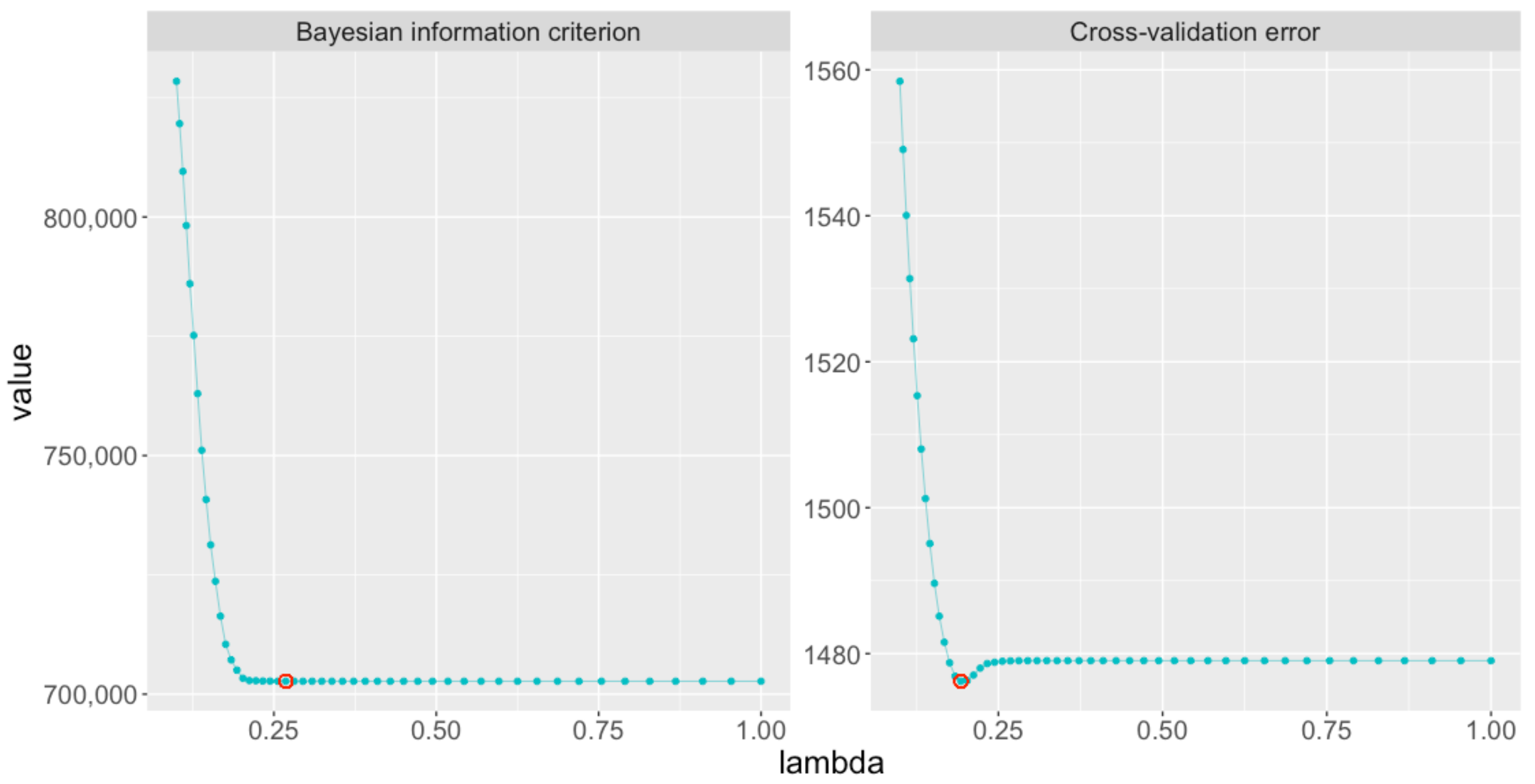
First, when we used BIC (with the warm start) to estimate the optimal value of
, we obtained
(see
Figure 7). Therefore, the estimated graph
is the solution of
jewel corresponding to this parameter. It has 3113 edges (about 2.7% of all possible edges), and all 483 vertices have a degree of at least 1.
When we used CV (with the warm start) to estimate the optimal value of
, we obtained
(see
Figure 7). We ran
jewel with this value of the regularization parameter. Resulting graph
has 7272 edges (about 6.2% of all possible edges) and all 483 vertices have a degree of at least 1. As, in this example
,
has more connections than
.
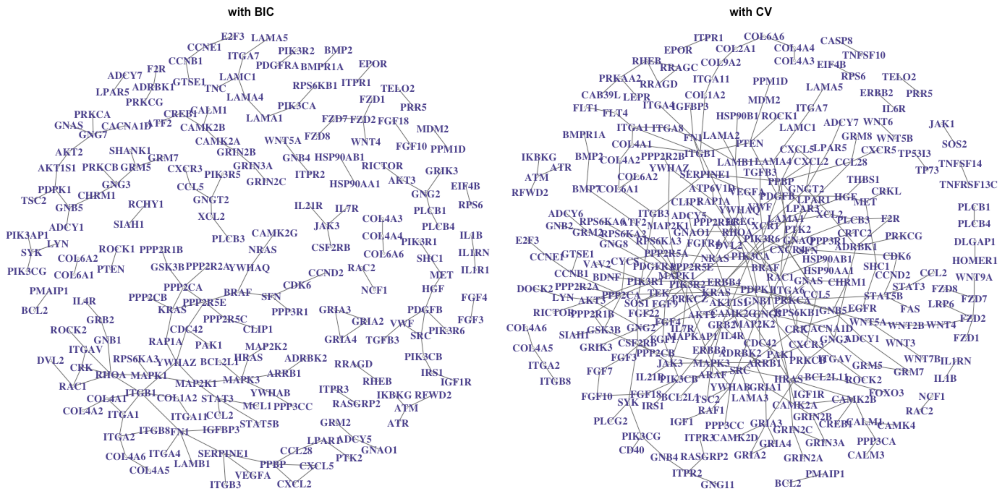
Then, to better understand the identified connections, we analyzed the
genes in the STRING database [
34]. STRING is a database of known and predicted protein–protein interactions that can be physical and functional and derived from lab experiments, known co-expression, and genomic context predictions and knowledge in the databases text mining. We limited the query to connections from “experiments” and “databases” as active interaction sources setting the minimum required interaction score to the highest value of 0.9. The resulting STRING network had 415 out of 483 vertices connected to any other node and 4134 edges.
We measured the number of connections common to our estimated network and the network from the STRING database. For each case,
Figure 8 shows the connections identified by
jewel that were present also in the STRING database. For
, we observed 170 edges in common, while for
, we had 297 common edges (see all the results summarized in
Table 3).
Although the number of edges in the intersection can be considered low at first sight, it is significant according to the hypergeometric test. Nevertheless, we should note two things: First, jewel seeks to identify conditional correlation among variables or equivalently linear relationships between two genes not mediated by other factors (i.e., other genes). Meanwhile, connections from the STRING database are not necessarily of such nature. Second, STRING contains general protein–protein interactions, i.e., interactions that are not necessarily present in the tissue/condition studied in used datasets. Therefore, we do not expect to identify mechanisms that might occur in other biological conditions (our gene expressions are glioblastoma).
However, we notice many groups of genes identified consistently, such as collagen alpha chains, ionotropic glutamate receptors, frizzled class receptors, interleukin 1 receptors, and fibroblast growth factors, collagen, and others. The biggest hubs in include PPP3CC (frequently underexpressed in gliomas), RCHY1 (vice versa, typically highly expressed in this condition), and IL4R (is associated with better survival rates). In , the biggest hubs are TNN (that is considered a therapeutic target since an increase in expression can suppress brain tumor growth), CALML6, and BCL-2 (that can block apoptosis, i.e., cell death, and therefore may influence tumor prognosis).
To conclude, jewel demonstrated its ability to identify connections from the gene expression microarray data. However, it is possible that the choice of the regularization parameter still deserves improvements to achieve better results.
4. Discussion
The proposed method jewel is a methodological contribution to the GGM inference in the context of multiple datasets. It provides a valid alternative if the user is interested only in the structure of the GGM and not in covariance estimation. The proposed method is easy to use with the R package jewel.
There are still some aspects that can be improved and constitute directions for future work. As the performance of any regularization method depends on the choice of the tuning parameter,
jewel could be improved with the better choice of
. For example, in [
24] the authors suggest quantile universal threshold,
, which is the upper
-quantile of the introduced zero-thresholding function under the null model. When not only the response vector but also the design matrix is random (as in
), bootstrapping within the Monte Carlo simulation can be used to evaluate
.
Moving to more methodological improvements, we can incorporate degree-induced weights into the minimization problem to account for the underlying graph’s hub structure. In this way, we could overcome the decrease in performance demonstrated by all analyzed methods. Furthermore, we can consider other grouping approaches as the neighbor-dependent synergy described in [
35]. Another possible improvement, when the underlying graphs are not the same across all the
K datasets, is to decompose
as a sum of two factors, one describing the common part and another the differences between the
K graphs, then add a second group Lasso penalty term to capture differences between the networks. Other intriguing improvements regard the incorporation of specific prior knowledge, which would lead to different initialization of the
matrix. For example, using variable screening procedures, i.e., a preliminary analysis of the input data that identifies connections that are not “important” with high probability, we can reduce the problem’s dimensionality. Other aspects concern implementing the block-diagonalization approach, i.e., identifying blocks in the underlying graph and perform independent execution of
jewel to each block. Such a choice does not influence performance but can significantly decrease the running time, especially if we parallelize the execution of
jewel to different blocks.
Finally, another point that might greatly impact the applications of
jewel to the analysis of gene expression has to do with the Gaussian assumption. Nowadays, RNA-seq data have become popular and are replacing the old microarray technology. However, RNA-seq are counts data. Therefore the Gaussian assumption does not hold. Methods such as
voom [
36] can be used to transform the RNA-seq data and stabilize the variance.
voom estimates the mean-variance relationship of the log-counts, generates a precision weight for each observation and enters these into the
limma [
37] empirical Bayes analysis pipeline. With this transformation, the RNA-seq can be analyzed using similar tools as for microarrays,
jewel included. As a more appealing alternative, one could develop a joint graphical approach in the context of count data, such as in [
38,
39,
40].


