Article

Logistic Biplot by Conjugate Gradient Algorithms and Iterated SVD

by
Jose Giovany Babativa-Márquez
1,2,* and
José Luis Vicente-Villardón
1
1
Department of Statistics, University of Salamanca, 37008 Salamanca, Spain
2
Facultad de Ciencias de la Salud y del Deporte, Fundación Universitaria del Área Andina, Bogotá 1321, Colombia
*
Author to whom correspondence should be addressed.
Mathematics 2021, 9(16), 2015; https://doi.org/10.3390/math9162015
Submission received: 24 June 2021 / Revised: 19 August 2021 / Accepted: 19 August 2021 / Published: 23 August 2021
(This article belongs to the Special Issue Multivariate Statistics: Theory and Its Applications)

Abstract

:
Multivariate binary data are increasingly frequent in practice. Although some adaptations of principal component analysis are used to reduce dimensionality for this kind of data, none of them provide a simultaneous representation of rows and columns (biplot). Recently, a technique named logistic biplot (LB) has been developed to represent the rows and columns of a binary data matrix simultaneously, even though the algorithm used to fit the parameters is too computationally demanding to be useful in the presence of sparsity or when the matrix is large. We propose the fitting of an LB model using nonlinear conjugate gradient (CG) or majorization–minimization (MM) algorithms, and a cross-validation procedure is introduced to select the hyperparameter that represents the number of dimensions in the model. A Monte Carlo study that considers scenarios with several sparsity levels and different dimensions of the binary data set shows that the procedure based on cross-validation is successful in the selection of the model for all algorithms studied. The comparison of the running times shows that the CG algorithm is more efficient in the presence of sparsity and when the matrix is not very large, while the performance of the MM algorithm is better when the binary matrix is balanced or large. As a complement to the proposed methods and to give practical support, a package has been written in the R language called BiplotML. To complete the study, real binary data on gene expression methylation are used to illustrate the proposed methods.

1. Introduction

In many studies, researchers have a binary multivariate data matrix and aim to reduce dimensions to investigate the structure of the data. For example, in the measurement of brand equity, a set of consumers evaluates the perceptions of quality, perceptions of value, or other brand attributes that can be represented in a binary matrix [1]; in the evaluation of the impact of public policies, the answers used to identify whether the beneficiaries have some characteristics or to identify if some economic or social conditions have changed from a baseline are usually binary [2,3,4]. Likewise, in biological research—and in particular in the analysis of genetic and epigenetic alterations—the amount of binary data has been increasing over time [5]. In these cases, classical methods to reduce dimensionality, such as principal component analysis (PCA), are not appropriate.
This problem has received considerable attention in the literature; consequently, different extensions of PCA have been proposed. From a probabilistic perspective, Collins et al. [6] provide a generalization of PCA to exponential family data using the generalized linear model framework. This approach suggests the possibility of having proper likelihood loss functions depending on the type of data.
Logistic PCA is the extension of the classic PCA method for binary data and was studied by Schein et al. [7] using the Bernoulli likelihood, where an alternating least squares method is used to estimate the parameters. De Leeuw [8] proposed the calculation of the maximum likelihood estimates of a PCA on the logit or probit scale, using a MM algorithm that iterates a sequence of weighted or unweighted singular value decompositions. Subsequently, Lee et al. [9] introduced sparsity to the loading vectors defined on the logit transform of the success probabilities of the binary observations and estimated the parameters using an iterative weighted least squares algorithm, but the algorithm is computationally too demanding to be useful when the data dimension is high. To solve this problem, a different method was proposed by Lee and Huang [10] using a combined algorithm with coordinate descent and MM to reduce the computational effort. More recently, Landgraf and Lee [11] proposed a formulation that does not require matrix factorization, and they use an MM algorithm to estimate the parameters of the logistic PCA model. Song et al. [12] proposed the fitting of a logistic PCA model using an MM algorithm across a non-convex singular value threshold to alleviate the overfitting issues. However, neither of these approaches provides a simultaneous representation of rows and columns to visualize the binary data set, similar to what is called a biplot for continuous data [13].
The biplot methods allow the simultaneous representation of the individuals and variables of a data matrix [14]. Biplots have proven to be very useful for analyzing multivariate continuous data [15,16,17,18,19] and have also been implemented to visualize the results of other multivariate techniques such as multidimensional scaling, MANOVA, canonical analysis, correspondence analysis, generalized bilinear models, and the HJ-Biplot, among many others [14,20,21,22,23,24].
In cases where the variables of the data matrix are not continuous, a classical linear biplot representation is not suitable. Gabriel [25] proposed the “bilinear regression” to fit a biplot for data with distributions from the exponential family, but the algorithm was not clearly established and was never used in practice. For multivariate binary data, Vicente-Villardon et al. [26] proposed a biplot called Logistic Biplot (LB), which is a dimension reduction technique that generalizes PCA to cope with binary variables and has the advantage of simultaneously representing individuals and variables. In the LB, each individual is represented by a point and each variable as directed vectors, and the orthogonal projection of each point onto these vectors predicts the expected probability that the characteristic occurs. The method is related to logistic regression in the same way that classical biplot analysis is related to linear regression. In the same way, as linear biplots are related to PCA, LB is related to Latent Trait Analysis (LTA) or Item Response Theory (IRT).
The authors estimate the parameters of the LB model by a Newton–Raphson algorithm, but this presents some problems in the presence of separation or sparsity. In [27], the method is extended using a combination of principal coordinates and standard logistic regression to approximate the LB model parameters in the genotype classification context and is called an external logistic biplot, but the procedure of estimation is quite inefficient for big data matrices. More recently, in [28], the external logistic biplot method was extended for mixed data types, but the estimation algorithm still has problems with big data matrices or in the presence of sparsity. Therefore, there is a clear need to extend the previous algorithms for the LB model because they are not very efficient and none of them present a procedure for choosing the number of dimensions of the final solution of the model.
In the context of supervised learning, some optimization methods have been successfully implemented for logistic regression. For example, Komarek and Moore [29] develops Truncated-Regularized Iteratively-Reweighted Least Squares (TR-IRLS) technique that implements a linear Conjugate Gradient (CG) to approximate the Newton direction. The algorithm is especially useful for large, sparse data sets because it is fast, accurate, robust to linear dependencies, and no data preprocessing is necessary. Furthermore, another of the advantages of the CG method is that it guarantees convergence in a maximum number of steps [30]. On the other hand, when the imbalance is extreme, this problem is known as the rare events problem or the imbalanced data problem, which presents several problems and challenges to existing classification algorithms [31]. Maalouf and Siddiqi [32] developed a method of Rare Event Weighted Logistic Regression (RE-WLR) for the classification of imbalanced data on large-scale data.
In this paper, we propose the estimation of the parameters of the LB model in two different ways: one of these is to use CG methods, and the other way is to use a coordinate descendent MM algorithm. In addition, we incorporate a cross-validation procedure to estimate the generalization error and thus choose the number of dimensions in the LB model.
Taking into account the latent variables and model specification that defines a LB, a simulation process is carried out that allows for the evaluation of the performance of the algorithms and their ability to identify the correct number of dimensions to represent the multivariate binary data matrix adequately. Besides the proposed methods, the BiplotML package [33] was written in R language [34] to give practical support to the new algorithms.
The paper is organized into the following sections. Section 2.1 presents the classical biplot for continuous data. Next, Section 2.2 presents the formulation of the LB model. Section 2.3 introduces the proposed adaptation of the CG algorithm and the coordinate descendent MM algorithm to fit the LB model. Section 2.4 describes the model selection procedure (number of dimensions) and introduces our formulation via simulated data. Section 3 presents the performance of the proposed models and an application using real data. Finally, Section 4 presents a discussion of the main results.

2. Materials and Methods

2.1. Biplot for Continuous Data

Classical biplot methods allow the combined visualization of the rows and columns of a data matrix X = x 1 , , x n T , with x i R p , i = 1 , , n being a vector of the observations of an individual i on p variables in low-dimensional space [13,14].
More generally, if r a n k ( X ) = r and the data are centered, given a positive integer k r , a biplot is an approximation
X = AB T + E ,
where A and B are matrices of rank k, and E is the matrix that contains the approximation errors. In this way, the matrix X can be graphically represented using markers (points or vectors) a 1 , , a n for its rows and b 1 , , b p for its columns, in such a way that the i j -th element of the matrix, x i j , is approximated by the inner product a i T b j , and the natural space of parameters is determined by Θ = A B T .
It is well known that we can reproduce exactly the matrix in dimension r using its singular value decomposition (SVD),
X = U Λ V T ,
where U = u 1 , , u r and V = v 1 , , v r are the matrices of left and right singular vectors and Λ is the r-dimensional diagonal matrix containing the singular values in decreasing order λ 1 λ r > 0 . It is also known that the low (k)-rank approximation for X is obtained from
Θ = U ( k ) Λ ( k ) V ( k ) T = AB T ,
where the subscript ( k ) stands for the first k columns of the matrix. We can define a biplot in the form of Equation (1) taking A = U ( k ) Λ ( k ) γ and B = V Λ ( k ) ( 1 γ ) , 0 γ 1 . Then, Θ = AB T minimizes the Frobenius norm
X Θ F 2 = i = 1 n x i a i 1 b 1 + + a i k b k 2 ,
for any value of γ . Note that, for example, if γ = 1 , A contains the coordinates of individuals on the principal components and B is the projection of the initial coordinate axis onto them. There are algorithms other than SVD used to calculate the markers as alternated regressions [13] or NIPALS [35].

2.2. Logistic Biplot

Let X = x 1 , , x n T be a binary matrix, with x i { 0 , 1 } p , i = 1 , , n and x i j B e r ( π ( θ i j ) ) , where π ( · ) is the inverse link function. In this paper, the logit link is used, π ( θ i j ) = 1 + e x p ( θ i j ) 1 , which represents the expected probability that the character j is present in individual i, the log-odds π ( θ i j ) is θ i j with θ i j = l o g π ( θ i j ) / ( 1 π ( θ i j ) ) , which corresponds to the natural parameter of the Bernoulli distribution expressed in an exponential family form. Using the probability distribution, we have P ( X i j = x i j ) = π ( θ i j ) x i j 1 π ( θ i j ) 1 x i j , and the loss function is obtained as the negative log likelihood
L Θ = i = 1 n j = 1 p x i j l o g ( π ( θ i j ) ) + ( 1 x i j ) l o g ( 1 π ( θ i j ) ) .
In this case, it is not appropriate to center the columns because the centered matrix will no longer be made up of elements equal to zero or one. Therefore, we extend the specification of the natural parameter space by introducing variable main effects or the column offset term μ for a model-based centering. The canonical parameter matrix Θ = θ 1 , , θ n T can be represented by a low-dimensional structure for some integer k r that satisfies θ i = μ + s = 1 k a i s b s , i = 1 , , n , which expressed in matrix form is written as
Θ = l o g i t Π = 1 n μ T + AB T ,
where 1 n is an n-dimensional vector of ones; μ = μ 1 , , μ p T ; A = a 1 , , a n T with a i R k , i = 1 , , n ; B = b 1 , , b k with b j R p , j = 1 , , k ; and Π = π Θ is the predicted matrix whose i j th element equals π ( θ i j ) . Now, Θ = l o g i t ( Π ) is a biplot in the logit scale and log-odds θ i j = μ j + a i T b j .
In addition to the canonical parameter matrix Θ , the hyperparameter k must also be estimated to select the LB model. In general, in dimensionality reduction methods, the choice of k is problematic and presents a risk of overfitting [36]. We propose the use of a completely unsupervised procedure based on cross-validation for LB model selection to counteract such overfitting. Cross-validation is operationally simple and allows the selection of the number of dimensions at the point where a numerical criterion is minimized, which will indicate that choosing more dimensions would lead to the overfitting of the model.
Once the parameters have been estimated, the geometry of the biplot regression allows us to obtain the direction vector g j that projects a row marker of A to predict the values in column j [21,26]. For example, to find the coordinates for a fixed probability π when k = 2 , we look for the point ( g j 1 , g j 2 ) that predicts π and that is on the biplot axis, i.e., on the line joining the points ( 0 , 0 ) and ( b j 1 , b j 2 ) , which is calculated as
g j 1 = ( l o g i t ( π ) μ j ) b j 1 s = 1 2 b j s 2 , g j 2 = ( l o g i t ( π ) μ j ) b j 2 s = 1 2 b j s 2 .
In the logistics biplot, as in the classic PCA biplot, all directions pass through the origin. In a PCA biplot for centered data, the origin represents the mean of each variable and the arrow shows the direction of increasing values. As the binary data cannot be centered (we keep the column offset term in the model), the origin does not represent any particular value of the probability. In the LB model, we represent the variables with arrows (segments) starting at the point that predicts 0.5 and ending at the point that predicts 0.75.

2.3. Parameter Estimation

Expressing the loss function given in (5) as L Θ = i = 1 n j = 1 p f ( θ i j ) and considering that the logit link function is used, π ( θ i j ) = ( 1 exp ( θ i j ) ) 1 , the gradient is
f ( θ i j ) = x i j 1 π ( θ i j ) π ( θ i j ) θ i j + ( 1 x i j ) 1 1 π ( θ i j ) ( 1 π ( θ i j ) ) θ i j = x i j ( 1 π ( θ i j ) ) ( 1 x i j ) π ( θ i j ) = π ( θ i j ) x i j .
The second derivative, 2 f ( θ i j ) = π ( θ i j ) ( 1 π ( θ i j ) ) is a quadratic function satisfying 0 2 f ( θ i j ) 1 / 4 as x i j has a Bernoulli distribution.

2.3.1. Estimation Using Nonlinear Conjugate Gradient Algorithms

Let L Θ be a matrix whose i j th element equals π ( θ i j ) x i j , which will be expressed in matrix form as
L Θ = Π X .
As the θ i j = μ j + a i T b j , then the L Θ function involves the matrices A and B through π ( θ i j ) = π ( μ j + a i T b j ) . In this way, it is also possible to calculate the partial derivatives with respect to μ , A , and B (see Appendix A):
L μ = Π X T 1 n
L A = Π X B
L B = Π X T A
For the model to be identifiable and to avoid the elements of B becoming too small due to changes in the scale of A and not due to changes in the log-likelihood, it is usually required that A T A = I k [9]. However, the maximum likelihood estimation of the model with this constraint tends to overfit the data [12]. In this paper, we use an approach that allows us to control the scale from the simultaneous updating of the parameters.
The initialization of the algorithm starts at point Θ 0 = 1 n μ 0 T + A 0 B 0 T , which can be configured by the user or by using a random initialization. For a random initialization, all elements of A 0 = a 1 0 , , a n 0 T , B 0 = b 1 0 , , b k 0 , and μ 0 can be sampled from the uniform distribution. We choose the first search direction d l T to be the steepest descent direction at the initial point Θ 0 ; then, a line search method is used to calculate the step-length parameter α l , and using a scalar β l , we define the rule for updating the direction based on the gradient at every iteration and thus simultaneously update μ , A , and B , thus updating the natural space of parameters Θ . The pseudocode is written formally in Algorithm 1.
Algorithm 1 CG Algorithm for fitting a LB model
Input  X
Output  μ , A , B
 1: Initialize μ 0 , A 0 , B 0
 2: Θ 0 = 1 n μ 0 T + A 0 B 0 T
 3: L 0 = L Θ 0
 4: d 0 = L 0
 5: l = 0
 6: repeat
 7:   Π l = π Θ l
 8:   α l = arg min α > 0 L Θ l + α d l
 9:   A l + 1 = A l + α l Π l X B l
10:   B l + 1 = B l + α l Π l X T A l
11:   μ l + 1 = μ l + α l Π l X T 1 n
12:   Θ l + 1 = 1 n μ l + 1 T + A l + 1 B l + 1 T
13:   L l + 1 = π Θ l + 1 X
14:  Compute β l + 1 according to one of the formulas given in (13)
15:   d l + 1 = L l + 1 + β l + 1 d l
16: until  L Θ l L Θ l + 1 / L Θ l < ϵ
This is a method that is considered to have low computational cost because each iteration only requires the evaluation of the gradient and the loss function, so it can become efficient in large data sets [37,38]. In this paper, we use four well-known formulas for the update direction: Fletcher–Reeves (FR), Polak–Ribiere–Polyak (PRP), Hestenes–Stiefel (HS), and Dai–Yuan (DY) [39,40,41,42], which can be written as
β l + 1 F R = L l + 1 2 L l 2 ; β l + 1 P R P = L l + 1 T Δ l L l 2 ; β l + 1 H S = L l + 1 T Δ l d l T Δ l ; β l + 1 D Y = L l + 1 2 d l T Δ l ,
where Δ l = L l + 1 L l , and · is the Euclidean norm. These methods have had modifications that combine the formulas [43,44,45,46,47,48,49] and that could be adapted to fit a LB model.
To achieve convergence in the implementation of the CG algorithm, one often requires the step-length obtained with a line search to be exact or satisfy the strong Wolfe conditions,
L Θ l L Θ l + α l d l c 1 α l L l T d l ,     L Θ l + α l d l T d l c 2 L l T d l ,
with 0 < c 1 < c 2 < 1 . As the FR method has been shown to be globally convergent under strong Wolfe line searches with c 2 < 1 / 2 [50,51], this condition ensures that all d l directions are descending directions from L .

2.3.2. Estimation Using Coordinate Descendent MM Algorithm

As the optimization problem is non-convex, we also use a MM algorithm to generate solutions that decrease with each iteration. The negative log-likelihood can be majorized by a quadratic function, and the majorized function can then be minimized iteratively.
According to Taylor’s theorem, and taking into account the fact that 2 f ( θ i j ) 1 / 4 , the loss functions of a single estimated natural parameter given in (5) are quadratically approximated at θ i j ( l ) by
f ( θ i j ) = x i j l o g ( π ( θ i j ) ) + ( 1 x i j ) l o g ( 1 π ( θ i j ) ) f ( θ i j ( l ) ) + ( π ( θ i j ( l ) ) x i j ) ( θ i j θ i j ( l ) ) + 1 2 π ( θ i j ( l ) ) ( 1 π ( θ i j ( l ) ) ) ( θ i j θ i j ( l ) ) 2 f ( θ i j ( l ) ) + ( π ( θ i j ( l ) ) x i j ) ( θ i j θ i j ( l ) ) + 1 8 ( θ i j θ i j ( l ) ) 2 = f ( θ i j ( l ) ) + 1 8 θ i j θ i j ( l ) + 4 ( π ( θ i j ( l ) ) x i j ) 2 2 ( π ( θ i j ( l ) ) x i j ) 2
= 1 8 θ i j θ i j ( l ) + 4 ( π ( θ i j ( l ) ) x i j ) 2 + C .       
Consequently, the loss function for the whole canonical matrix of parameters is majorized by
L Θ 1 8 i = 1 n j = 1 p θ i j z i j ( l ) 2 + C ,
where C is a constant that does not depend on Θ , and z i j ( l ) = θ i j ( l ) + 4 x i j π ( θ i j ( l ) ) .
Let Z l be the matrix whose i j th element equals z i j ( l ) . According to [52], the iteratively weighted least squares algorithm can be used as an upper bound for a quadratic function, which allows for the minimization of the majorization function as
L Θ 1 8 Θ Z l F 2 + C ,
and thus the majorized function to be minimized is written as
min μ , A , B 1 n μ T + AB T Z l F 2 .
In this case, the parameters are estimated sequentially. The algorithm is based on the coordinate descent optimization of the majorized function. When fixing AB T in Equation (19), μ can be estimated by the vector of mean scores of each column of matrix Z l , μ = 1 n Z l 1 n . In this way, the optimization problem becomes min A , B AB T P Z l F 2 where P = I 1 n 1 n 1 n T . To initialize Θ 0 = 1 n μ 0 T + A 0 B 0 T , we use A 0 = a 1 0 , , a n 0 T ; B 0 = b 1 0 , , b k 0 . μ 0 can be sampled from the uniform distribution. Algorithm 2 presents the pseudocode of this process.
Algorithm 2 Coordinate descendent MM algorithm for fitting a LB model
Input  X
Output  μ , A , B
 1: Initialize μ 0 , A 0 , B 0
 2: Θ 0 = 1 n μ 0 T + A 0 B 0 T
 3: l = 0
 4: repeat
 5:    Π l = π Θ l
 6:    Z l = Θ l + 4 X Π l
 7:    μ ( l + 1 ) = 1 n Z l 1 n
 8:    Z l + 1 c = P Z l , with P = I 1 n 1 n 1 n T
 9:    Z l + 1 c = U Λ V T
10:     A l + 1 = U Λ
11:   B l + 1 = V
12:   Θ l + 1 = 1 n μ l + 1 T + A l + 1 B l + 1 T
13: until  L Θ l L Θ l + 1 / L Θ l < ϵ

2.4. Simulated and Real Data

2.4.1. Real Data

We used data from the Genomic Determinants of Sensitivity in Cancer 1000 (GDSC1000) [5]. The database contains 926 tumor cell lines with comprehensive measurements of point mutation, CNA, methylation, and gene expression. For the purpose of illustrating the methods, the methylation data were used, and to facilitate the interpretation of the results, three types of cancer were included: breast invasive carcinoma (BRCA), lung adenocarcinoma (LUAD), and skin cutaneous melanoma (SKCM).

2.4.2. Simulation Process

The data sets were simulated from a latent variables model with different levels of sparsity and with a low-dimensional structure according to the model presented in Equation (6). To generate the binary matrix X , we used the procedure presented in Algorithm 3.
Algorithm 3 Algorithm to simulate a binary data matrix
Input  n , p , k , D .
Output  X , Θ , μ , A , B
1: B =   b 1 , , b k with b j N ( 0 , 1 ) , j = 1 , , k .
2: procedure Gram–Schmidt algorithm
3:   B T B = I k
4: end procedure
5: μ = μ 1 , , μ p T with μ i = l n D 1 D
6: A N ( 0 , I k )
7: Θ = 1 n μ T + AB T
8: X = x 1 , , x n T , with x i j B e r ( π ( θ i j ) ) , π ( θ i j ) = 1 + e x p ( θ i j ) 1 .
The offset term μ was used to control the sparsity, while the log-odds Θ was defined to have a low-dimensional structure.

2.5. Model Performance Assessment

To evaluate the performance of the CG algorithm and the MM algorithm, we used the training error, which is defined as the average misclassification rate when using the low-dimensional structure generated by the LB model with the training set. Each algorithm provided an estimate of μ , A , and B . We used the predicted probability matrix Π = π 1 n μ T + A B T to select p thresholds, 0 < δ j < 1 ,   j = 1 , , p —one for each column of X —and then perform the binary classification. As the data matrices could be imbalanced, we used the training error defined as Balanced Accuracy (BACC), which is most appropriate in these cases [53,54]
B A C C = 1 2 T P T P + F N + T N T N + F P ,
where T P is the number of true positives, T N is the number of true negatives, F P is the number of false positives, and F N is the number of false negatives.
To decide the classification rule from the predicted value, a threshold must be selected for each variable. This threshold value can be selected by minimizing the BACC rate for each variable in the training set and then applying the rule to a test set.
As the training error can be an optimistic measure of the misclassification rate, we also used a cross-validation procedure that allowed for the testing of the models; thus, we used a test data set that was independent of the training data set. As in the supervised models, cross-validation was used to keep track of the overfitting of the model. In our case, the LB model is a non-supervised method to reduce the dimensionality, and cross-validation helps to find the number of dimensions to maintain [36,55,56,57]. The procedure allowed us to estimate the value of the hyperparameter k to avoid overfitting and evaluate the capacity of the different estimation algorithms to identify the low-dimensional space.
As in PCA, we expect that a few dimensions would reproduce the original data (binary) as well as possible; then, we excluded some observed values, fit the model without those values, and calculated the expected probabilities for the missing data. Using the rule of classifying a missing value as being present if the fitted probability is higher than a threshold δ j , we imputed the selected missing data and calculated the classification. We performed this procedure M times for different values of k, and select the value that minimizes the generalization error.
More formally, we used the exclusion pattern proposed by Wold [55], which consists of a selected sequence of elements x i j being left out using a diagonal pattern and treated as missing values; in this way, we avoided the problems of excluding a complete row or column as described in [36,57]. Let W be a binary matrix, where w i j = 0 if the value is excluded (belongs to the validation set) and w i j = 1 is not (belongs to the training set). The minimization problem thus became
min μ , A , B l o g ( p ( X ; Θ , W ) ) = l o g i = 1 n j = 1 p p ( x i j ; θ i j ) w i j = i = 1 n j = 1 p w i j x i j l o g ( π ( θ i j ) ) + ( 1 x i j ) l o g ( 1 π ( θ i j ) ) .
The loss function now depends only on the training set. Solving the problem with one of the proposed algorithms, we created a matrix of expected probabilities Π = π ( Θ ) . Then, x ^ i j = 1 when π ( Θ ) > δ j , and x ^ i j = 0 otherwise, where 0 < δ j < 1 is the threshold for minimizing the BACC rate for variable j in the training set. We used the elements of X ^ when w i j = 0 to calculate the BACC. This procedure was performed M times, and the generalization error given by the cross-validation was calculated using the mean of the BACC; we considered M = 7 folds as in [57].
We also measured the models’ ability based on each algorithm to recover the log-odds Θ ; for this, we used the relative mean squared error (RMSE), defined as
R M S E ( Θ ) = Θ Θ ^ F 2 Θ F 2 .
where Θ is the true parameter and Θ ^ is estimated by the LB model using one of the proposed algorithms.

3. Results

3.1. Monte Carlo Study

Binary matrices were simulated with n = 100 ,   300 ,   500 ; p = 50 ,   100 ; k = 3 ; and D = 0.5 ,   0.3 ,   0.2 ,   0.1 , where the parameter D represents the proportion of ones in matrix X . The different sparsity levels were simulated to check if the performance with the algorithms to find the low-dimensional structure was affected for this reason. The combinations of n, p, k, and D generated the different scenarios; in each scenario, R matrices were simulated independently, and the measures were calculated to evaluate the performance of the algorithms. Finally, the mean of the cross-validation error (cv error) was calculated, as well as the mean of the training error (BACC) and the mean of the relative mean squared error (RMSE) with their respective standard errors. We used a value of R = 30 that generated standard errors less than 1 % in the estimation of the BACC and cv error.
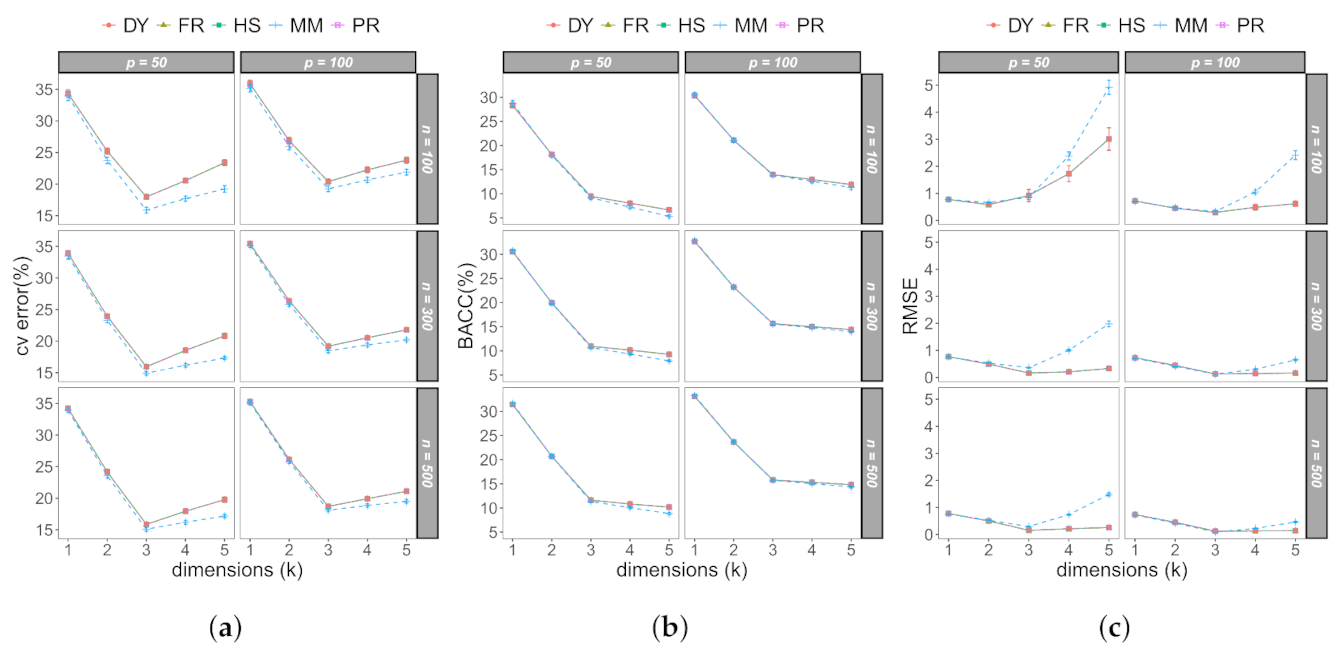
Figure 1a presents the cross-validation error of the algorithms based on the conjugate gradient and the MM algorithm when the matrix X is balanced. From the cv error, we can see that all models began to overfit when k > 3 , so the five estimation methods identified the three underlying dimensions for all balanced scenarios that were simulated. Figure 1b shows the Balanced Accuracy (BACC); it is highlighted that the slope decelerated when the three underlying dimensions were reached in the matrix, and thus an elbow criterion could be used as a signal of the number of dimensions to choose. Finally, Figure 1c shows the estimation of the relative mean squared error (RMSE) for the matrix Θ ; we see that the algorithms based on the conjugate gradient and the MM algorithm showed similar results when the number of dimensions was less than or equal to 3. Whereas, when the model had more than the three predefined dimensions in the simulation, the algorithms based on the conjugate gradient presented a lower RMSE than the MM algorithm, although, for a fixed value of p, these gaps closed as n increased.
Figure 2a–c show the cross-validation errors when the data are imbalanced with D = 0.3 ,   0.2 , and 0.1 , respectively. In all the scenarios studied, it is observed that the error was minimized when the number of underlying dimensions in the space of the variables was reached, so our method identified that a value of k = 3 in the LB model was appropriate to avoid overfitting. As this occurred with all imbalanced data sets, then we see that the level of dispersion does not affect the performance of the algorithms in terms of correctly finding the low-dimensional space.
The training error for imbalanced data sets with different levels of sparsity is shown in Figure 3a–c. In all the studied scenarios, it is observed that the percentage of loss in the training error stabilized from the third dimension. In this way, the different algorithms allowed the low-dimensional space to be appropriately selected using the elbow method.
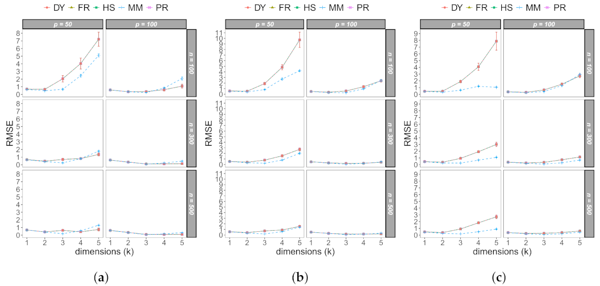
The RMSE of the estimation of the log-odds Θ for the different levels of sparsity is shown in Figure 4a–c; we can see that the algorithms presented similar performances. In the scenarios of n = 100 and p = 50 , it is observed that the RMSE increased notably when the number of dimensions was greater than 3, so there were some important gaps between the two approaches, although these differences decreased as the value of p or the value of n increased.
On the other hand, the computational performance of the algorithms was measured on a computer with an Intel Core i7-3517U processor with 6 GB of RAM. Table 1 shows the the running time in seconds with 100 replications for k = 3 and a stopping criterion of ϵ = 10 4 . We see that the performances of the different algorithms were competitive, and they converged relatively quickly when the maximum of the absolute changes of the estimated parameters in two subsequent iterations was less than 10 4 . In general, it is observed that the CPU times of the CG algorithms were similar and presented a better performance than the MM algorithm when p = 50 and the sparsity level began to be high ( D 0.2 ), or when n = 100 , p = 100 , and D = 0.1 . In the other cases, the MM algorithm performed better, especially when n and p increased, resulting in up to six times faster performance than CG algorithms in balanced scenarios when n = 500 and p = 100 .

3.2. Application

To apply the proposed methodology, we used data from the Genomic Determinants of Sensitivity in Cancer 1000 (GDSC1000) [5]. The database contains 926 tumor cell lines with comprehensive measurements of point mutation, CNA, methylation, and gene expression. To illustrate the methods, the methylation data were used, and to facilitate the interpretation of the results, three types of cancer were included: breast invasive carcinoma (BRCA), lung adenocarcinoma (LUAD), and skin cutaneous melanoma (SKCM).
We performed preprocessing to sort the data sets and separate the methylation information into one data set. After preprocessing, the methylation dataset has 160 rows and 38 variables, each variable is a CpG island located in the gene promoter area. In this case, code 1 indicates a high level of methylation, and 0 indicates a low level; approximately 27 % of the binary data matrix are ones.
Figure 5 shows the cross-validation error and training error using the conjugate gradient algorithms and the coordinate descendent MM algorithm. If k = 0 , the model (6) only considered the term μ , meaning that Θ = 1 n μ T , where μ j is the proportion of ones in column j and was used as a reference to observe the performance of the algorithms when more dimensions were included by incorporating the row and column markers, Θ = 1 n μ T + AB T .
The cross-validation error was minimized in three dimensions for the four formulas (FR, HS, PR, and DY) based on the CG algorithm, so k = 3 was the appropriate value to avoid overfitting when using these methods of estimation. When using the MM algorithm, it was found that the LB model generated overfitting for k > 2 , so using two dimensions in the LB model is suitable when using this estimation method.
An advantage of using a biplot approach is that it allows for a simultaneous representation of rows and columns, which are plotted with points and directed vectors, respectively. Figure 6 shows the biplot obtained for the methylation data using the Fletcher–Reeves conjugate gradient algorithm; the vectors of the variables are represented by arrows (segments) that start at the point that predicts 0.5 and end at the point that predicts 0.75 . Therefore, short vectors indicate a rapid increase in probability and the orthogonal projection of the row markers on the vector approximates the probability of finding high levels of methylation in the cell line.
The position of the segment, which corresponds to the point that predicts a probability of 0.5, can start any side around the origin. For example, in Figure 6, the variable DUSP22 points to the origin, when doing the orthogonal projection of the points in the direction of the vector, most of them will be projected after the reference point where the segment starts; this means that almost all cell lines of the three groups have high fitted probabilities of having high levels of methylation in that variable.
The cell lines are separated into three clearly identified clusters. In the BRCA type of cancer, variables such as NAPRT1, THY1, or ADCY4 are directed towards the positive part of dimension 1 and therefore have a greater probability of presenting high levels of methylation. The LUAD cell lines are located in the negative part of dimension 2, so these have a high propensity to present high levels of methylation in variables such as HIST1H2BH, ZNF382, and XKR6. Finally, the cell lines for the SKCM cancer type are located in the negative part of dimension 1 and have a greater probability of presenting high levels of methylation in variables such as LOC100130522, CHRFAM7A, or DHRS4L2.
Table 2 shows the rate of correct classifications for each variable using the measures of sensitivity and specificity; these measures allowed us to determine if the model exhibited a good classification for the two types of data in each variable. Sensitivity measured the true positives rate, specificity measured the true negatives rate, and the global measure corresponded to the total rate of correct classifications for each variable.
In general, the model with three dimensions and using the CG algorithm with the FR formula generated high values for sensitivity; only the GSTT1 gene presented a relatively low sensitivity, with 72% true positives. Regarding specificity, the LOC391322 gene obtained the lowest true negatives rate, with 80.9%. Thus, the results of the model are satisfactory.

4. Conclusions and Discussion

The Logistic Biplot (LB) model is a dimensionality reduction technique that generalizes the PCA to deal with binary variables and has the advantage of simultaneously representing individuals and variables (biplot).
In this paper, we propose and develop a methodology to estimate the parameters of the LB model using nonlinear conjugate gradient algorithms or the descending coordinate MM algorithm. For the selection of the LB model, we have incorporated a cross-validation procedure that allows the choice of the number of dimensions of the model in order to counteract overfitting.
As a complement to the proposed methods and to give practical support, a package has been written in the R language called BiplotML package [33], which is available from CRAN; this is a valuable tool that enables the application of the proposed algorithms to data analysis in every scientific field. Our contribution is important because we provide alternatives to solve some problems encountered in the LB model in the presence of sparsity or a big data matrix [23,26,27,28]. Additionally, a procedure is presented that allows the choice of the number of dimensions, which until now had not been investigated for an LB model.
The proposed algorithms are iterative and have the property that the loss function decreases with each iteration. To study the properties of the proposed algorithms to fit a LB model, low rank data sets with k = 3 and different levels of sparsity were generated for n = 100 ,   300 ,   500 rows and p = 50 ,   100 columns. The accuracy of the algorithms was measured using the training error, generalization error (cv-error), and mean square error (RMSE) of the log-odds. According to the Monte Carlo study, we established that the cross-validation criterion is successful in the estimation of the hyperparameter of the number of dimensions. This allows the model to be specified and thus avoid overfitting; in this way, we obtain the best performance of the proposed algorithms in terms of recovering the underlying low rank structure.
The comparison of the running times showed that the algorithms converge quickly. The CG algorithm is more efficient when the matrices are sparse and not very large, while the performance of the MM algorithm is better when the number of rows and columns tends to increase; thus, it is preferable for large matrices.
Finally, we used real data on gene expression methylation to show our approach. The LB model allowed us to carry out a simultaneous projection between rows and columns, where a grouping of three classes was observed, formed by the cell lines of the three types of cancer analyzed. Furthermore, the vectors that represented the variables allowed us to identify those cell lines that were more likely to achieve high levels of methylation in the different genes.

Author Contributions

Conceptualization, J.G.B.-M. and J.L.V.-V.; methodology, J.G.B.-M. and J.L.V.-V.; software, J.G.B.-M.; validation, J.L.V.-V. and J.G.B.-M.; formal analysis, J.G.B.-M. and J.L.V.-V.; investigation, J.G.B.-M.; resources, J.L.V.-V.; data curation, J.G.B.-M.; writing—original draft preparation, writing—review and editing, J.G.B.-M. and J.L.V.-V.; visualization, J.G.B.-M.; supervision, J.L.V.-V.; funding acquisition, J.G.B.-M. All authors have read and agreed to the published version of the manuscript.

Funding

This research received no external funding.

Institutional Review Board Statement

Ethical review and approval were waived for this paper due to GDSC1000 being open data and completely anonymized; thus, the privacy of any patient data is not compromised.

Informed Consent Statement

Any research article describing a study involving humans should contain this statement.

Data Availability Statement

The data analyzed in this paper can be found at https://www.cancerrxgene.org/gdsc1000/GDSC1000_WebResources/Home.html (accessed on 14 May 2021).

Conflicts of Interest

The authors declare no conflict of interest.

Abbreviations

The following abbreviations are used in this manuscript:
LBLogistic Biplot
MMMajorization–Minimization
CGConjugate Gradient
PCAPrincipal Component Analysis
BACCBalanced Accuracy
RMSERelative Mean Squared Error
SVDSingular Value Decomposition
NIPALSNonlinear estimation by Iterative Partial Least Square
LTALatent Trait Analysis
IRTItem Response Theory
RE-WLRRare Event Weighted Logistic Regression
TR-IRLSTruncated Regularized Iteratively Re-weighted Least Squares

Appendix A. Derivatives

The loss function given in (5) can be expressed as L Θ = i = 1 n j = 1 p f ( θ i j ) , where π ( θ i j ) = ( 1 exp ( θ i j ) ) 1 and θ i j = μ j + s = 1 k a i s b j s = μ j + a i T b j , thereby
f ( θ i j ) a i s = x i j 1 π ( θ i j ) π ( θ i j ) a i s + ( 1 x i j ) 1 1 π ( θ i j ) + ( 1 π ( θ i j ) ) a i s
since π ( θ i j ) a i s = b j s π ( θ i j ) ( 1 π ( θ i j ) ) so that ( 1 π ( θ i j ) ) a i s = b j s π ( θ i j ) ( 1 π ( θ i j ) ) then
f ( θ i j ) a i s = b j s ( π ( θ i j ) x i j ) , s = 1 , , k .
Analogously, we obtain
f ( θ i j ) b j s = x i j 1 π ( θ i j ) π ( θ i j ) b j s + ( 1 x i j ) 1 1 π ( θ i j ) ( 1 π ( θ i j ) ) b j s
= a i s ( π ( θ i j ) x i j ) , s = 1 , , k ,
where π ( θ i j ) b j s = a i s π ( θ i j ) ( 1 π ( θ i j ) ) . Finally, the offset term
f ( θ i j ) μ j = x i j 1 π ( θ i j ) π ( θ i j ) μ j + ( 1 x i j ) 1 1 π ( θ i j ) ( 1 π ( θ i j ) μ j
= ( π i j x i j ) .
In matrix terms, we can write it as
L μ = Π X T 1 n ; L A = ( Π X ) B ; L B = ( Π X ) T A .

References

  1. Keller, K. Strategic Brand Management: Building, Measuring, and Managing Brand Equity; Pearson/Prentice Hall: Hoboken, NJ, USA, 2008. [Google Scholar]
  2. Murray, D.; Pals, S.; Blitstein, J. Design and Analysis of Group-Randomized Trials: A Review of Recent Methodological Developments. Am. J. Public Health 2004, 94, 423–432. [Google Scholar] [CrossRef]
  3. Moerbeek, M.; Breukelen, G.; Berger, M. Optimal Experimental Designs for Multilevel Logistic Models. J. R. Stat. Soc. Ser. D Stat. 2001, 50, 17–30. [Google Scholar] [CrossRef]
  4. Moerbeek, M.; Maas, C. Optimal Experimental Designs for Multilevel Logistic Models with Two Binary Predictors. Commun. Stat. Theory Methods 2005, 34. [Google Scholar] [CrossRef]
  5. Iorio, F.; Knijnenburg, T.A.; Vis, D.J.; Bignell, G.R.; Menden, M.P.; Schubert, M.; Aben, N.; Gonçalves, E.; Barthorpe, S.; Lightfoot, H.; et al. A landscape of pharmacogenomic interactions in cancer. Cell 2016, 166, 740–754. [Google Scholar] [CrossRef] [PubMed] [Green Version]
  6. Collins, M.; Dasgupta, S.; Schapire, R.E. A generalization of principal components analysis to the exponential family. In Advances in Neural Information Processing Systems 14; The MIT Press: Cambridge, MA, USA, 2001; pp. 617–624. [Google Scholar]
  7. Schein, A.I.; Saul, L.K.; Ungar, L.H. A Generalized Linear Model for Principal Component Analysis of Binary Data. In Proceedings of the 9th International Workshop on Artificial Intelligence and Statistics, Key West, FL, USA, 3–6 January 2003; Volume 38. [Google Scholar]
  8. De Leeuw, J. Principal component analysis of binary data by iterated singular value decomposition. Comput. Stat. Data Anal. 2006, 50, 21–39. [Google Scholar] [CrossRef]
  9. Lee, S.; Huang, J.Z.; Hu, J. Sparse logistic principal components analysis for binary data. Ann. Appl. Stat. 2010, 4, 1579–1601. [Google Scholar] [CrossRef] [Green Version]
  10. Lee, S.; Huang, J. A coordinate descent MM algorithm for fast computation of sparse logistic PCA. Comput. Stat. Data Anal. 2013, 62, 26–38. [Google Scholar] [CrossRef]
  11. Landgraf, A.J.; Lee, Y. Dimensionality reduction for binary data through the projection of natural parameters. J. Multivar. Anal. 2020, 180, 104668. [Google Scholar] [CrossRef]
  12. Song, Y.; Westerhuis, J.A.; Smilde, A.K. Logistic principal component analysis via non-convex singular value thresholding. Chemom. Intell. Lab. Syst. 2020, 204, 104089. [Google Scholar] [CrossRef]
  13. Gabriel, K.R. The biplot graphic display of matrices with application to principal component analysis 1. Biometrika 1971, 58, 453–467. [Google Scholar] [CrossRef]
  14. Gower, J.C.; Lubbe, S.G.; Le Roux, N.J. Understanding Biplots; John Wiley and Sons: Hoboken, NJ, USA, 2011. [Google Scholar]
  15. Scrucca, L. Graphical tools for model-based mixture discriminant analysis. Adv. Data Anal. Classif. 2014, 8, 147–165. [Google Scholar] [CrossRef] [Green Version]
  16. Groenen, P.J.; Le Roux, N.J.; Gardner-Lubbe, S. Spline-based nonlinear biplots. Adv. Data Anal. Classif. 2015, 9, 219–238. [Google Scholar] [CrossRef]
  17. Kendal, E.; Sayar, M. The stability of some spring triticale genotypes using biplot analysis. J. Anim. Plant Sci. 2016, 26, 754–765. [Google Scholar]
  18. Amor-Esteban, V.; Galindo-Villardón, M.P.; García-Sánchez, I.M. A multivariate proposal for a national corporate social responsibility practices index (NCSRPI) for international settings. Soc. Indic. Res. 2019, 143, 525–560. [Google Scholar] [CrossRef]
  19. González-García, N.; Nieto-Librero, A.B.; Vital, A.L.; Tao, H.J.; González-Tablas, M.; Otero, Á.; Galindo-Villardón, P.; Orfao, A.; Tabernero, M.D. Multivariate analysis reveals differentially expressed genes among distinct subtypes of diffuse astrocytic gliomas: Diagnostic implications. Sci. Rep. 2020, 10, 1–12. [Google Scholar] [CrossRef]
  20. Galindo Villardón, M.P. Una alternativa de representación simultánea: HJ-Biplot. Questiio 1986, 10, 13–23. [Google Scholar]
  21. Gower, J.C.; Hand, D.J. Biplots; CRC Press: Boca Raton, FL, USA, 1995; Volume 54. [Google Scholar]
  22. Greenacre, M.; Blasius, J. Multiple Correspondence Analysis and Related Methods; Chapman and Hall/CRC: London, UK, 2006. [Google Scholar]
  23. Hernández-Sánchez, J.C.; Vicente-Villardón, J.L. Logistic biplot for nominal data. Adv. Data Anal. Classif. 2017, 11, 307–326. [Google Scholar] [CrossRef] [Green Version]
  24. Cubilla-Montilla, M.; Nieto-Librero, A.B.; Galindo-Villardón, M.P.; Torres-Cubilla, C.A. Sparse HJ Biplot: A New Methodology via Elastic Net. Mathematics 2021, 9, 1298. [Google Scholar] [CrossRef]
  25. Gabriel, K.R. Generalised Bilinear Regression. Biometrika 1998, 85, 689–700. [Google Scholar] [CrossRef]
  26. Vicente-Villardon, J.; Galindo-Villardon, M.; Blazquez-Zaballos, A. Logistic Biplots. In Multiple Correspondence Analysis and Related Methods; Chapman-Hall: London, UK, 2006; Chapter 23; pp. 503–521. [Google Scholar]
  27. Demey, J.; Vicente Villardon, J.L.; Galindo Villardón, M.P.; Zambrano, A. Identifying molecular markers associated with classification of genotypes by External Logistic Biplots. Bioinformatics 2008, 24, 2832–2838. [Google Scholar] [CrossRef] [PubMed] [Green Version]
  28. Vicente-Villardón, J.L.; Hernández-Sánchez, J.C. External Logistic Biplots for Mixed Types of Data. In Advanced Studies in Classification and Data Science; Springer: New York, NY, USA, 2020; pp. 169–183. [Google Scholar]
  29. Komarek, P.; Moore, A.W. Fast Robust Logistic Regression for Large Sparse Datasets with Binary Outputs. In Proceedings of the Ninth International Workshop on Artificial Intelligence and Statistics, Key West, FL, USA, 3–6 January 2003; pp. 163–170. [Google Scholar]
  30. Lewis, J.M.; Lakshmivarahan, S.; Dhall, S. Dynamic Data Assimilation: A Least Squares Approach; Cambridge University Press: Cambridge, UK, 2006; Volume 13. [Google Scholar]
  31. King, G.; Zeng, L. Logistic Regression in Rare Events Data. Political Anal. 2001, 9, 137–163. [Google Scholar] [CrossRef] [Green Version]
  32. Maalouf, M.; Siddiqi, M. Weighted logistic regression for large-scale imbalanced and rare events data. Knowl. Based Syst. 2014, 59, 142–148. [Google Scholar] [CrossRef]
  33. Babativa-Marquez, J.G. Package BiplotML: Biplots Estimation with Machine Learning Algorithms. Available online: https://cran.r-project.org/package=BiplotML (accessed on 24 June 2021).
  34. R Core Team. R: A Language and Environment for Statistical Computing; R Foundation for Statistical Computing: Vienna, Austria, 2020. [Google Scholar]
  35. Wold, H. Estimation of principal components and related models by iterative least squares. In Multivariate Analysis; Academic Press: NewYork, NY, USA, 1966; pp. 391–420. [Google Scholar]
  36. Owen, A.B.; Perry, P.O. Bi-cross-validation of the SVD and the nonnegative matrix factorization. Ann. Appl. Stat. 2009, 3, 564–594. [Google Scholar] [CrossRef] [Green Version]
  37. Pytlak, R. Conjugate Gradient Algorithms in Nonconvex Optimization; Springer Science & Business Media: Berlin, Germany, 2008; Volume 89. [Google Scholar]
  38. Nocedal, J.; Wright, S. Numerical Optimization; Springer Science & Business Media: Berlin, Germany, 2006. [Google Scholar]
  39. Fletcher, R.; Powell, M.J. A rapidly convergent descent method for minimization. Comput. J. 1963, 6, 163–168. [Google Scholar] [CrossRef]
  40. Polak, E.; Ribiere, G. Note sur la convergence de méthodes de directions conjuguées. ESAIM Math. Model. Numer. Anal. Model. Math. Anal. Numer. 1969, 3, 35–43. [Google Scholar] [CrossRef]
  41. Polyak, B.T. The conjugate gradient method in extremal problems. USSR Comput. Math. Math. Phys. 1969, 9, 94–112. [Google Scholar] [CrossRef]
  42. Dai, Y.H.; Yuan, Y. A nonlinear conjugate gradient method with a strong global convergence property. SIAM J. Optim. 1999, 10, 177–182. [Google Scholar] [CrossRef] [Green Version]
  43. Dai, Y.H.; Yuan, Y. An efficient hybrid conjugate gradient method for unconstrained optimization. Ann. Oper. Res. 2001, 103, 33–47. [Google Scholar] [CrossRef]
  44. Zhang, L.; Zhou, W.; Li, D.H. A descent modified Polak–Ribière–Polyak conjugate gradient method and its global convergence. IMA J. Numer. Anal. 2006, 26, 629–640. [Google Scholar] [CrossRef]
  45. Andrei, N. A hybrid conjugate gradient algorithm for unconstrained optimization as a convex combination of Hestenes-Stiefel and Dai-Yuan. Stud. Inform. Control 2008, 17, 57. [Google Scholar]
  46. Yuan, G.; Zhang, M. A modified Hestenes-Stiefel conjugate gradient algorithm for large-scale optimization. Numer. Funct. Anal. Optim. 2013, 34, 914–937. [Google Scholar] [CrossRef]
  47. Liu, J.; Li, S. New hybrid conjugate gradient method for unconstrained optimization. Appl. Math. Comput. 2014, 245, 36–43. [Google Scholar] [CrossRef]
  48. Dong, X.L.; Liu, H.W.; He, Y.B.; Yang, X.M. A modified Hestenes–Stiefel conjugate gradient method with sufficient descent condition and conjugacy condition. J. Comput. Appl. Math. 2015, 281, 239–249. [Google Scholar] [CrossRef]
  49. Yuan, G.; Wei, Z.; Yang, Y. The global convergence of the Polak–Ribiere–Polyak conjugate gradient algorithm under inexact line search for nonconvex functions. J. Comput. Appl. Math. 2019, 362, 262–275. [Google Scholar] [CrossRef]
  50. Al-Baali, M. Descent property and global convergence of the Fletcher—Reeves method with inexact line search. IMA J. Numer. Anal. 1985, 5, 121–124. [Google Scholar] [CrossRef]
  51. Dai, Y.; Yuan, Y.X. Convergence properties of the Fletcher-Reeves method. IMA J. Numer. Anal. 1996, 16, 155–164. [Google Scholar] [CrossRef]
  52. Kiers, H.A. Weighted least squares fitting using ordinary least squares algorithms. Psychometrika 1997, 62, 251–266. [Google Scholar] [CrossRef]
  53. Velez, D.R.; White, B.C.; Motsinger, A.A.; Bush, W.S.; Ritchie, M.D.; Williams, S.M.; Moore, J.H. A balanced accuracy function for epistasis modeling in imbalanced datasets using multifactor dimensionality reduction. Genet. Epidemiol. Off. Publ. Int. Genet. Epidemiol. Soc. 2007, 31, 306–315. [Google Scholar] [CrossRef]
  54. Wei, Q.; Dunbrack, R.L., Jr. The role of balanced training and testing data sets for binary classifiers in bioinformatics. PLoS ONE 2013, 8, e67863. [Google Scholar] [CrossRef] [Green Version]
  55. Wold, S. Cross-validatory estimation of the number of components in factor and principal components models. Technometrics 1978, 20, 397–405. [Google Scholar] [CrossRef]
  56. Gabriel, K.R. Le biplot-outil d’exploration de données multidimensionnelles. J. Soc. Fr. Stat. 2002, 143, 5–55. [Google Scholar]
  57. Bro, R.; Kjeldahl, K.; Smilde, A.K.; Kiers, H. Cross-validation of component models: A critical look at current methods. Anal. Bioanal. Chem. 2008, 390, 1241–1251. [Google Scholar] [CrossRef] [PubMed]
Figure 1. Model selection and performance with balanced data. (a) Cross-validation error. (b) Training error. (c) RMSE.
Mathematics 09 02015 g001
Figure 2. Cross-validation error plot for imbalanced data sets with different levels of sparsity. (a) D = 0.3. (b) D = 0.2. (c) D = 0.1.
Mathematics 09 02015 g002
Figure 3. Training error plot for unbalanced data sets with different levels of sparsity. (a) D = 0.3. (b) D = 0.2. (c) D = 0.1.
Mathematics 09 02015 g003
Figure 4. RMSE of estimating Θ for imbalanced data sets with different levels of sparsity. (a) D = 0.3. (b) D = 0.2. (c) D = 0.1.
Mathematics 09 02015 g004
Figure 5. Cross-validation plots for CG algorithms and the coordinate descendent MM algorithm with methylation data. (a) FR. (b) HS. (c) PR. (d) DY. (e) MM.
Mathematics 09 02015 g005
Figure 6. Logistic biplot using a Fletcher–Reeves conjugate gradient algorithm for methylation data.
Mathematics 09 02015 g006
Table 1. Running time in seconds to estimate the LB model with k = 3 and ϵ = 10 4 .
npDDYFRHSPRMM
100500.129.930.129.929.9166.1
300500.184.685.485.085.3276.3
500500.1141.2141.5141.9141.1356.3
1001000.158.257.857.958.6115.1
3001000.1168.6167.4168.9169.4155.3
5001000.1302.4279.6330.8322.3215.5
100500.230.130.130.330.160.8
300500.2102.8103.1102.5100.8133.3
500500.2141.7159.3142.4141.9140.1
1001000.262.458.463.658.635.7
3001000.2169.8169.0168.4168.967.3
5001000.2283.0288.0281.9283.199.5
100500.330.130.630.230.436.6
300500.386.286.686.286.260.1
500500.3143.1143.2143.0143.999.3
1001000.358.759.058.858.826.8
3001000.3170.5170.5170.3169.750.1
5001000.3284.2284.5284.4284.677.3
100500.530.231.132.630.927.6
300500.587.198.787.586.955.8
500500.5145.6144.6145.4144.8103.0
1001000.558.758.959.259.218.8
3001000.5170.8171.2171.0171.130.2
5001000.5286.4327.9290.6341.656.4
Table 2. Sensitivity and specificity for each variable when fitting the LB model with k = 3 and a CG-FR algorithm.
VariableSensitivitySpecificityGlobal
GSTM197.194.896.2
C1orf70100.0100.0100.0
DNM3100.094.996.2
COL9A2100.0100.0100.0
VAR5100.094.395.6
VAR6100.088.691.2
THY1100.095.896.9
VAR8100.093.695.0
DNAH10100.0100.0100.0
VAR10100.090.892.5
DHRS4L2100.088.891.2
ADCY4100.098.398.8
CHRFAM7A100.092.494.4
VAR14100.099.199.4
FAM174B100.094.896.2
VAR16100.099.199.4
VAR17100.086.387.5
ARL17A100.098.699.4
HOXB8100.098.298.8
LOC100130522100.089.391.9
ZNF714100.0100.0100.0
ZNF38297.994.695.6
VAR23100.096.597.5
FRZB100.099.199.4
VAR25100.094.795.0
TBX1100.098.398.8
LOC391322100.080.981.2
GSTT172.087.180.0
VAR29100.096.697.5
FILIP1L97.193.694.4
VAR31100.097.598.1
HIST1H2BH100.089.792.5
DUSP22100.098.499.4
VAR3495.097.596.9
XKR6100.093.295.0
NAPRT196.987.589.4
VAR3795.895.695.6
VAR3897.798.398.1
Publisher’s Note: MDPI stays neutral with regard to jurisdictional claims in published maps and institutional affiliations.

