Dynamical Behavior Analysis of a Time-Delay SIRS-L Model in Rechargeable Wireless Sensor Networks

Abstract

The traditional SIRS virus propagation model is used to analyze the malware propagation behavior of wireless rechargeable sensor networks (WRSNs) by adding a new concept: the low-energy status nodes. The SIRS-L model has been developed in this article. Furthermore, the influence of time delay during the charging behavior of the low-energy status nodes needs to be considered. Hopf bifurcation is studied by discussing the time delay that is chosen as the bifurcation parameter. Finally, the properties of the Hopf bifurcation are explored by applying the normal form theory and the center manifold theorem.

1. Introduction

With the development and application of communication technology and sensor technology, wireless sensor networks (WSNs) have come into being. WSNs are widely used globally, such as in the military industry, agricultural production, ecological monitoring, disaster warning, and infrastructure status monitoring [1]. Due to the self-organized network of WSNs, sensor nodes are vulnerable to various attacks in the process of information transmission [2,3,4,5,6,7,8,9,10]. Thus, it is of practical significance to prevent and deal with malicious attacks in WSNs.

The characteristics of WSNs can be listed as follows: adapting wireless communication, the topology being able to be changed dynamically, the security mechanism being imperfect, and the energy of nodes being limited, etc. Thus, the security of wireless sensor networks is facing great challenges. The attacks against sensor network nodes can be roughly divided into the following types: network worms, bots, and Trojans, among others [11,12,13,14]. Most malware attacks in WSNs mainly aim at paralyzing them or losing their power. In order to overcome the defect of short life cycle of WSNs, wireless rechargeable sensor networks (WRSNs) have been developed and have caught more attention. Consequently, a relatively special attack has appeared to against the nodes’ power, namely, the denial of charge (DOC) [15]. The prevention and control of malware spread in WRSNs have become a hot issue.

The propagation mechanism of malware is similar to that of viruses in biological groups. Many scholars have made great contributions to malware propagation dynamics. In the beginning, the spread of malware mainly focuses on the traditional Internet. For example, Zou et al. put forward the worm propagation models represented by SI (susceptible–infected), SIS (susceptible–infected–susceptible), and SIR (susceptible–infected–recovered) [16,17,18,19]. These studies lay a foundation for the later studies on the propagation behavior of malware in WSNs. However, it is worth noting that there are some differences between WSNs and the traditional Internet: (1) Because of their topological structure, the communication range of WSNs has physical limitations. (2) The limited energy characteristics lead to uneven communication capabilities. (3) The link-layer access conflict and avoidance mechanism of WSNs sharing wireless channel also introduces space-time correlation for the propagation dynamics of WSNs. (4) WSNs have a high degree of self-organization. Therefore, it is of great significance to study the malware propagation model in WSNs, which has been proposed in recent years. For example, Tanachaiwiwat began to study the propagation behavior of network worms in 2009 [20]. Khayam et al. used signal processing technology to study the propagation model of worms in 2006 [21]. Furthermore, the SEIR (susceptible–exposed–infected–recovered) model is adapted to study the spread of malware [22], while the SEIRS-V (susceptible–exposed–infected–recovered–susceptible and vaccinated) model explores the application of Hopf bifurcation during the malware spreading [23,24]. With the development, the research on WRSNs was pushed forward recently [25,26,27,28,29,30,31], considering the new concept of L (low-energy status) nodes. It is worth noting that the transition from the low-energy status nodes to the normal status nodes is called charging. At present, there are many charging methods for WRSNs, such as unmanned aerial vehicle (UAV) charging [32].

The related techniques and modeling basis of this paper mainly refer to the papers in

Table 1. Related research on the modeling and analysis of this paper.

Authors	Model	Characteristics	Reference Content
Zhu et al. [33]	SIRS (susceptible–infected–recovered–susceptible)	The authors put forward the time delay of the immune validity; the SIRS model is applied to WSNs analysis.	SIRS model is taken as the premise of modeling; the SIRS-L model considering the low-energy state nodes is proposed in this paper.
Zhang et al. [23]	SEIRS-V (susceptible–exposed–infected-recovered–susceptible and vaccinated)	Time delay is applied to SEIRS-V model.	It provides the analysis reference of Hopf bifurcation and the corresponding mathematical processing method.
Liu et al. [25]	SIS-L (susceptible–infected–susceptible–low-energy status)	It first proposes the low-energy state nodes and combines them into the research of WSRNs.	It provides a theoretical basis for the low-energy status modeling.
Liu et al. [26]	SIAS-L (susceptible–infected–anti-malware–susceptible–low-energy status)	The status of anti-malware is proposed and the optimal strategy is considered.	It provides a theoretical basis for the low-energy status modeling.
Liu et al. [29]	SIS-L (susceptible–infected–susceptible–low-energy status)	Time delay is considered for the first time in the model with the low-energy state nodes. However, the bifurcation is not discussed.	It provides a theoretical reference for time-delay analysis and the feasibility in modeling.

:

In order to promote the study of virus dynamics in WRSNs, the modeling in this paper is mainly based on the SIRS (susceptible–infected–recovered–susceptible) infectious disease model. Combined with the charging delay in WRSNs, the bifurcation in the process of charging needs to be considered. Therefore, the general contributions of this paper are as follows:

• Establishing the SIRS-L (susceptible–infected–recovered–susceptible–low-energy) model.
• The equilibrium solutions of the SIRS-L model are obtained, and the basic reproductive number R0 is defined through the regeneration matrix [34].
• Revealing of the stability of the SIRS-L model when the charging delay is ignored.
• The variation of the solutions of the characteristic equation are discussed if the charging delay is considered through the theory in [35], and the occurrence conditions of Hopf bifurcation are figured out.
• The properties of the Hopf bifurcation are explored by applying the normal form theory and the center manifold theorem [36].

The content of this paper is organized as follows: In Section 2, we establish the SIRS-L (susceptible–infected–recovered–susceptible–low-energy) model combined with the concept of low-energy nodes and the charging delay; in Section 3, the equilibrium points analysis and the corresponding Hopf bifurcation conditions are presented; the properties of the Hopf bifurcation are given in Section 4; the simulation analysis are revealed in Section 5; the conclusions are given in Section 6.

2. Modeling

On the basis of the classical SIRS model, we obtained the SIRS-L model as follows (1), with the parameters being explained in

Table 2. Interpretation of the model parameters.

S(t)	The Susceptible Nodes
I(t)	The infected nodes
R(t)	The recovered nodes
LS(t)	The low-energy status susceptible nodes
LI(t)	The low-energy status infected nodes
LR(t)	The low-energy status recovered nodes
N(t)	Total number of nodes
∧	Injection rate of new sensor nodes
${\alpha }_1$	Diffusion rate of malware
${\alpha }_2$	Self-healing rate of the infected nodes
${\alpha }_3$	Recovery rate of the infected nodes
${\alpha }_4$	Immune rate of the susceptible nodes
${\alpha }_5$	Immune failure rate of the recovered nodes; the recovered nodes will be re-exposed to the malware and may be infected again
${\beta }_1$	Low-energy node conversion rate, which is to describe the process of the general nodes dropping to the low-energy nodes
${\beta }_2$	Charging success rate
b	Node deactivation rate

:

$$\begin{array}{ll}\frac{dS\left(t\right)}{dt}\hfill & =\wedge -\frac{{\alpha }_{1}S\left(t\right)I\left(t\right)}{N\left(t\right)}-{\alpha }_{4}S\left(t\right)-{\beta }_{1}S\left(t\right)-bS\left(t\right)+{\alpha }_{2}I\left(t\right)+{\alpha }_{5}R\left(t\right)+{\beta }_{2}LS\left(t-\tau \right)\hfill \\ \frac{ dI\left(t\right)}{dt}\hfill & =\frac{{\alpha }_{1}S\left(t\right)I\left(t\right)}{N\left(t\right)}-{\alpha }_{2}I\left(t\right)-bI\left(t\right)-{\beta }_{1}I\left(t\right)-{\alpha }_{3}I\left(t\right)+{\beta }_{2}LI\left(t-\tau \right)\hfill \\ \frac{ dR\left(t\right)}{dt}\hfill & ={\alpha }_{3}I\left(t\right)+{\alpha }_{4}S\left(t\right)-bR\left(t\right)-{\beta }_{1}R\left(t\right)-{\alpha }_{5}R\left(t\right)+{\beta }_{2}LR\left(t-\tau \right)\hfill \\ \frac{dLS\left(t\right)}{dt}\hfill & ={\beta }_{1}S\left(t\right)-bLS\left(t\right)-{\beta }_{2}LS\left(t-\tau \right)\hfill \\ \frac{dLI\left(t\right)}{dt}\hfill & ={\beta }_{1}I\left(t\right)-bLI\left(t\right)-{\beta }_{2}LI\left(t-\tau \right)\hfill \\ \frac{dLR\left(t\right)}{dt}\hfill & ={\beta }_{1}R\left(t\right)-bLR\left(t\right)-{\beta }_{2}LR\left(t-\tau \right)\hfill \end{array}$$

(1)

The following formula is obtained through the injection rate and the deactivation rate: $\frac{dN\left(t\right)}{dt}=\wedge -bN\left(t\right)$. Therefore, we can obtain $N(\infty )=\frac{\wedge }{b}$ if the total number of nodes is stable. In order to make the analysis more clearer, the system (1) is simplified as follows (2) with the meaning $x\left(t\right)=\frac{X\left(t\right)}{N(\infty )}$, where $x\left(t\right)={\left(s\left(t\right), i\left(t\right), r\left(t\right), ls\left(t\right), li\left(t\right), lr\left(t\right)\right)}^T$ and $X\left(t\right)={\left(S\left(t\right), I\left(t\right), R\left(t\right), LS\left(t\right), LI\left(t\right), LR\left(t\right)\right)}^T$. Thus, $x\left(t\right)$ represents the proportion of nodes in the system (1).

$$\begin{array}{l}\frac{ds\left(t\right)}{dt}=b-{\alpha }_{1}s\left(t\right)i\left(t\right)-{\alpha }_{4}s\left(t\right)-{\beta }_{1}s\left(t\right)-bs\left(t\right)+{\alpha }_{2}i\left(t\right)+{\alpha }_{5}r\left(t\right)+{\beta }_{2}ls\left(t-\tau \right)\\ \frac{di\left(t\right)}{dt}={\alpha }_{1}s\left(t\right)i\left(t\right)-{\alpha }_{2}i\left(t\right)-bi\left(t\right)-{\beta }_{1}i\left(t\right)-{\alpha }_{3}i\left(t\right)+{\beta }_{2}li\left(t-\tau \right)\\ \frac{dr\left(t\right)}{dt}={\alpha }_{3}i\left(t\right)+{\alpha }_{4}s\left(t\right)-br\left(t\right)-{\beta }_{1}r\left(t\right)-{\alpha }_{5}r\left(t\right)+{\beta }_{2}lr\left(t-\tau \right)\\ \frac{dls\left(t\right)}{dt}={\beta }_{1}s\left(t\right)-bls\left(t\right)-{\beta }_{2}ls\left(t-\tau \right)\\ \frac{dli\left(t\right)}{dt}={\beta }_{1}i\left(t\right)-bli\left(t\right)-{\beta }_{2}li\left(t-\tau \right)\\ \frac{dlr\left(t\right)}{dt}={\beta }_{1}r\left(t\right)-blr\left(t\right)-{\beta }_{2}lr\left(t-\tau \right)\end{array}$$

(2)

3. Local Stability and Analysis of Hopf Bifurcation

The disease-free solution $e_0$ and endemic solution $e_{+}$ of the system (2) can be obtained as follows:

$$\begin{array}{l}{e}_0\left(s_0,i_0,r_0,l{s}_0,l{i}_0,l{r}_0\right)\\ =(\frac{b}{{\alpha }_4+{\beta }_1+b-{\beta }_2\epsilon -\frac{{\alpha }_4{\alpha }_5}{b+{\beta }_1+{\alpha }_5-{\beta }_2\epsilon }}, 0, \frac{{\alpha }_{4}b}{\left({\alpha }_4+{\beta }_1+b-{\beta }_2\epsilon \right)\left(b+{\beta }_1+{\alpha }_5-{\beta }_2\epsilon \right)-{\alpha }_4{\alpha }_5},\\ \frac{\epsilon b}{{\alpha }_4+{\beta }_1+b-{\beta }_2\epsilon -\frac{{\alpha }_4{\alpha }_5}{b+{\beta }_1+{\alpha }_5-{\beta }_2\epsilon }}, 0, \frac{\epsilon {\alpha }_{4}b}{\left({\alpha }_4+{\beta }_1+b-{\beta }_2\epsilon \right)\left(b+{\beta }_1+{\alpha }_5-{\beta }_2\epsilon \right)-{\alpha }_4{\alpha }_5}),\end{array}$$

(3)

$$\begin{array}{l}{e}_{+}\left(s_{+},i_{+},r_{+},l{s}_{+},l{i}_{+},l{r}_{+}\right)\\ =(\frac{{\alpha }_2+b+{\beta }_1+{\alpha }_3-{\beta }_2\epsilon }{{\alpha }_1} ,\frac{\left(b+{\beta }_1+{\alpha }_5-{\beta }_2\epsilon \right)r_{+}-{\alpha }_4{s}_{+}}{{\alpha }_3} , \frac{({\alpha }_2-{\alpha }_1{s}_{+}){\alpha }_4{s}_{+}+{\alpha }_3\left({\alpha }_4+{\beta }_1+b-{\beta }_2\epsilon \right)s_{+}-{\alpha }_{3}b}{({\alpha }_2-{\alpha }_1{s}_{+})\left(b+{\beta }_1+{\alpha }_5-{\beta }_2\epsilon \right)+{\alpha }_3{\alpha }_5} ,\\ \frac{\epsilon \left({\alpha }_2+b+{\beta }_1+{\alpha }_3-{\beta }_2\epsilon \right)}{{\alpha }_1}, \frac{\epsilon \left[\left(b+{\beta }_1+{\alpha }_5-{\beta }_2\epsilon \right)r_{+}-{\alpha }_4{s}_{+}\right]}{{\alpha }_3}, \frac{\epsilon \left[({\alpha }_2-{\alpha }_1{s}_{+}){\alpha }_4{s}_{+}+{\alpha }_3\left({\alpha }_4+{\beta }_1+b-{\beta }_2\epsilon \right)s_{+}-{\alpha }_{3}b\right]}{({\alpha }_2-{\alpha }_1{s}_{+})\left(b+{\beta }_1+{\alpha }_5-{\beta }_2\epsilon \right)+{\alpha }_3{\alpha }_5}),\end{array}$$

(4)

where $\epsilon =\frac{{\beta }_1}{b+{\beta }_2}$.

The basic reproductive number R0 is obtained through the next generation matrix method [34].

Set:

$$F=\left(\begin{array}{cc}{\alpha }_{1}s\left(t\right)& 0\\ 0& 0\end{array}\right),$$

(5)

and

$$V=\left(\begin{array}{cc}{\alpha }_2+b+{\beta }_1+{\alpha }_3& -{\beta }_2\\ -{\beta }_1& b+{\beta }_2\end{array}\right).$$

(6)

Thus,

$$R0=\rho \left(F{V}^{-1}\right)=\frac{{\alpha }_1{s}_0\left(b+{\beta }_2\right)}{\left({\alpha }_2+b+{\beta }_1+{\alpha }_3\right)\left(b+{\beta }_2\right)-{\beta }_1{\beta }_2}.$$

(7)

It can be found that if $R0>1$, the model (2) has the unique endemic solution $e_{+}$. By linearization technique, the characteristic matrix of system (2) about $e_{+}$ can be obtained as follows.

$$J\left(e_{+}\right)=\left(\begin{array}{cccccc}\lambda -a_{11}& -a_{12}& -b_{13}{e}^{-\lambda \tau }& -b_{14}{e}^{-\lambda \tau }& 0& 0\\ -a_{21}& \lambda -a_{22}& 0& 0& -b_{25}{e}^{-\lambda \tau }& 0\\ -a_{31}& -a_{32}& \lambda -a_{33}-b_{33}{e}^{-\lambda \tau }& 0& 0& -b_{36}{e}^{-\lambda \tau }\\ -a_{41}& 0& 0& \lambda -a_{44}-b_{44}{e}^{-\lambda \tau }& 0& 0\\ 0& -a_{52}& 0& 0& \lambda -a_{55}-b_{55}{e}^{-\lambda \tau }& 0\\ 0& 0& -a_{63}& 0& 0& \lambda -a_{66}-b_{66}{e}^{-\lambda \tau }\end{array}\right).$$

where

$$\begin{gathered} a_{11}=-{\alpha }_1{i}_{+}-{\alpha }_4-{\beta }_1-b,\hspace{1em}{a}_{12}=-{\alpha }_1{s}_{+}+{\alpha }_2,\hspace{1em}{a}_{13}={\alpha }_5, b_{14}={\beta }_2 \\ {a}_{21}={\alpha }_1{i}_{+}, a_{22}={\alpha }_1{s}_{+}-{\alpha }_2-b-{\beta }_1-{\alpha }_3,\hspace{1em}{b}_{25}={\beta }_2 \\ {a}_{31}={\alpha }_4, a_{32}={\alpha }_3, a_{33}=-b-{\beta }_1-{\alpha }_5, b_{36}={\beta }_2 \\ {a}_{41}={\beta }_1, a_{44}=-b, b_{44}=-{\beta }_2 \\ {a}_{52}={\beta }_1, a_{55}=-b, b_{55}=-{\beta }_2 \\ {a}_{63}={\beta }_1, a_{66}=-b, b_{66}=-{\beta }_2. \end{gathered}$$

The characteristic equation of the model (2) at $e_{+}$ is shown as:

$$\begin{array}{l}{\lambda }^6+A_5{\lambda }^5+A_4{\lambda }^4+A_3{\lambda }^3+A_2{\lambda }^2+A_1\lambda +A_0\\ +\left(B_5{\lambda }^5+B_4{\lambda }^4+B_3{\lambda }^3+B_2{\lambda }^2+B_1\lambda +B_0\right)e^{-\lambda \tau }\\ +\left(C_4{\lambda }^4+C_3{\lambda }^3+C_2{\lambda }^2+C_1\lambda +C_0\right)e^{-2\lambda \tau }\\ +\left(D_3{\lambda }^3+D_2{\lambda }^2+D_1\lambda +D_0\right)e^{-3\lambda \tau }=0.\end{array}$$

(8)

The detailed representations of $X_n\left(X=A,B,C,D;n=1,2,3\dots \right)$ are given in Appendix A.

Firstly, we study the local stability of system (2) at $e_{+}$ when $\tau =0$.

If $\tau =0$, Equation (8) can be rebuilt as:

$${\lambda }^6+E_5{\lambda }^5+E_4{\lambda }^4+E_3{\lambda }^3+E_2{\lambda }^2+E_1\lambda +E_0=0,$$

(9)

where

$$\begin{array}{l}{E}_5=A_5+B_5, E_4=A_4+B_4+C_4, E_3=A_3+B_3+C_3+D_3,\\ E_2=A_2+B_2+C_2+D_2, E_1=A_1+B_1+C_1+D_1, E_0=A_0+B_0+C_0+D_0.\end{array}$$

The following formulas can be obtained:

$$\{\begin{array}{l}{△}_1 = E_5,\hfill \\ {△}_2 = \left|\begin{array}{cc}{E}_5& 1\\ E_3& E_4\end{array}\right|,\hfill \\ {△}_3 = \left|\begin{array}{ccc}{E}_5& 1& 0\\ E_3& E_4& E_5\\ E_1& E_2& E_3\end{array}\right|,\hfill \\ {△}_4 = \left|\begin{array}{cccc}{E}_5& 1& 0& 0\\ E_3& E_4& E_5& 1\\ E_1& E_2& E_3& E_4\\ 0& E_0& E_1& E_2\end{array}\right|,\hfill \\ {△}_5 = \left|\begin{array}{ccccc}{E}_5& 1& 0& 0& 0\\ E_3& E_4& E_5& 1& 0\\ E_1& E_2& E_3& E_4& E_5\\ 0& E_0& E_1& E_2& E_3\\ 0& 0& 0& E_0& E_1\end{array}\right|,\hfill \\ {△}_6 = E_0{△}_5.\hfill \end{array}$$

(10)

If hypothesis (H1) $E_5,E_4,E_3,E_2,E_1,E_0>0, {△}_1$, ${△}_2$, ${△}_3$, ${△}_4$, ${△}_5$, ${△}_6>0$ and $\tau =0$, in Equation (10) holds, and all the characteristic solutions of Equation (9) are negative. Thus, $e_{+}$ is locally asymptotically stable under the theory of the Hurwitz criterion.

Then, we begin to consider the change of the characteristic solutions of Equation (9) when the charging time delay $\mathsf{\tau }$ is introduced.

If $\tau >0$, multiplying $e^{\lambda \tau }$ on both sides of Equation (8), we can obtain the following equation:

$$B_5{\lambda }^5+B_4{\lambda }^4+B_3{\lambda }^3+B_2{\lambda }^2+B_1\lambda +B_0$$

(11)

Referring to the processing method of the paper [35], let $\lambda$ = iω (ω > 0) be the root of Equation (11). After separating the imaginary and real parts, we obtain

$$\{\begin{array}{c}{F}_1\cos \tau \omega -F_2\sin \tau \omega +F_3=G_1\sin 2\tau \omega +G_2\cos 2\tau \omega \\ F_4\sin \tau \omega -F_5\cos \tau \omega +F_6=G_1\cos 2\tau \omega -G_2\sin 2\tau \omega \end{array},$$

(12)

where

$$\begin{array}{l}{F}_1=-{\omega }^6+A_4{\omega }^4-A_2{\omega }^2+A_0+C_4{\omega }^4-C_2{\omega }^2+C_0,\\ F_2=A_5{\omega }^5-A_3{\omega }^3+A_1\omega +C_3{\omega }^3-C_1\omega ,\\ F_3=B_4{\omega }^4-B_2{\omega }^2+B_0,\\ F_4=A_5{\omega }^5-A_3{\omega }^3+A_1\omega -C_3{\omega }^3+C_1\omega ,\\ F_5=-{\omega }^6+A_4{\omega }^4-A_2{\omega }^2+A_0-C_4{\omega }^4+C_2{\omega }^2-C_0,\\ F_6=B_5{\omega }^5-B_3{\omega }^3+B_1\omega ,\\ G_1=D_3{\omega }^3-D_1\omega ,\\ G_2=D_2{\omega }^2-D_0.\end{array}$$

Squaring and adding the two Equations in Equation (12), we obtain

$${\left(F_1\cos \tau \omega -F_2\sin \tau \omega +F_3\right)}^2+{\left(F_4\sin \tau \omega -F_5\cos \tau \omega +F_6\right)}^2=G_1{}^2+G_2{}^2$$

(13)

Because of $\sin \tau \omega =\pm \sqrt{1-{\cos }^2\tau \omega }$, the following two cases are discussed:

Case 1: If $\sin \tau \omega =\sqrt{1-{\cos }^2\tau \omega }$, Equation (13) could be represented as follows:

$${\left(F_1\cos \tau \omega -F_2\sqrt{1-{\cos }^2\tau \omega }+F_3\right)}^2+{\left(F_4\sqrt{1-{\cos }^2\tau \omega }-F_5\cos \tau \omega +F_6\right)}^2=G_1{}^2+G_2{}^2$$

(14)

Equation (14) can be calculated as follows:

$$H_4{\cos }^4\tau \omega +H_3{\cos }^3\tau \omega +H_2{\cos }^2\tau \omega +H_1\cos \tau \omega +H_0=0,$$

(15)

where

$$\begin{array}{l}{H}_4={\left(F_1{}^2+F_5{}^2-F_2{}^2-F_4{}^2\right)}^2+4{\left(F_4{F}_5-F_1{F}_2\right)}^2,\\ H_3=(F_1{F}_3+F_5{F}_6)({F_1}^2+{F_5}^2-{F_2}^2-{F_4}^2)+8(F_4{F}_5-F_1{F}_2)(F_4{F}_6-F_2{F}_3),\\ H_2=4{\left(F_1{F}_3+F_5{F}_6\right)}^2-4{\left(F_4{F}_5-F_1{F}_2\right)}^2+4{\left(F_4{F}_6-F_2{F}_3\right)}^2\\ +2\left(F_1{}^2+F_5{}^2-F_2{}^2-F_4{}^2\right)\left(F_2{}^2+F_3{}^2+F_4{}^2+F_6{}^2-G_1{}^2-G_2{}^2\right),\\ H_1=4{\left(F_2{}^2+F_3{}^2+F_4{}^2+F_6{}^2-G_1{}^2-G_2{}^2\right)}^2\left(F_1{F}_3+F_5{F}_6\right)\\ -8\left(F_4{F}_5-F_1{F}_2\right)\left(F_4{F}_6-F_2{F}_3\right),\\ H_0={\left(F_2{}^2+F_3{}^2+F_4{}^2+F_6{}^2-G_1{}^2-G_2{}^2\right)}^2-4{\left(F_4{F}_6-F_2{F}_3\right)}^2.\end{array}$$

Let $\cos \tau \omega =y,$ and the following equation can be obtained:

$$f\left(y\right)=y^4+\frac{H_3}{H_4}{y}^3+\frac{H_2}{H_4}{y}^2+\frac{H_1}{H_4}y+\frac{H_0}{H_4},$$

(16)

and

$$\dot{f}\left(y\right)=4y^3+3\frac{H_3}{H_4}{y}^2+2\frac{H_2}{H_4}{y}^1+\frac{H_1}{H_4}.$$

(17)

Set

$$y^3+I_2{y}^2+I_1{y}^1+I_0=0,$$

(18)

where

$$I_2=\frac{3H_3}{4H_4}, I_1=\frac{H_2}{2H_4}, I_0=\frac{H_1}{4H_4}.$$

The following solutions can be calculated:

$$\begin{array}{l}{y}_1={\sigma }_1-\frac{\frac{I_1}{3}-\frac{I_2{}^2}{9}}{{\sigma }_1}-\frac{I_2}{3},\\ y_2=\frac{\frac{I_1}{3}-\frac{I_2{}^2}{9}}{2{\sigma }_1}-\frac{I_2}{3}-\frac{{\sigma }_1}{2}-\frac{\sqrt{3}\frac{\frac{I_1}{3}-\frac{I_2{}^2}{9}}{{\sigma }_1}+{\sigma }_1}{2}\mathrm{i},\\ y_3=\frac{\frac{I_1}{3}-\frac{I_2{}^2}{9}}{2{\sigma }_1}-\frac{I_2}{3}-\frac{{\sigma }_1}{2}+\frac{\sqrt{3}\left(\frac{\frac{I_1}{3}-\frac{I_2{}^2}{9}}{{\sigma }_1}+{\sigma }_1\right)}{2}\mathrm{i},\end{array}$$

(19)

where

$${\sigma }_1={\left(\sqrt{{\left(\frac{I_2{}^3}{27}-\frac{I_1{I}_2}{6}+\frac{I_0}{2}\right)}^2+{\left(\frac{I_1}{3}-\frac{I_2{}^2}{9}\right)}^3}-\frac{I_0}{2}-\frac{I_2{}^3}{27}+\frac{I_1{I}_2}{6}\right)}^{\frac{1}{3}}.$$

Then, the expression of $\cos \tau \omega$ can be obtained as $f_1\left(\omega \right)=\cos \tau \omega ;$ combined with Equation (13), we can obtain $f_2\left(\omega \right)=\sin \tau \omega .$ A function concerning ω can be obtained by

$$f_1{}^2\left(\omega \right)+f_2{}^2\left(\omega \right)=1.$$

(20)

Thus, (H2) Equation (20) has finite positive roots ${\omega }_{1i}$ ($i=1,2,\dots ,n$). The corresponding time delay can be obtained as follows:

$${\tau }_{1i}^{\left(j\right)}=\frac{1}{{\omega }_{1i}}arccos{f}_1\left({\omega }_{1i}\right)+\frac{2j\pi }{{\omega }_{1i}}, i=1,2,\dots ,n. j=0,1,2\dots$$

(21)

Case 2: If $\sin \tau \omega =-\sqrt{1-{\cos }^2\tau \omega }$, Equation (13) could be represented as follows:

$${\left(F_1\cos \tau \omega -F_2\sqrt{1-{\cos }^2\tau \omega }+F_3\right)}^2+{\left(F_4\sqrt{1-{\cos }^2\tau \omega }-F_5\cos \tau \omega +F_6\right)}^2=G_1{}^2+G_2{}^2.$$

(22)

Similar to Case 1, a function concerning ω can be obtained by

$$f_3{}^2\left(\omega \right)+f_4{}^2\left(\omega \right)=1.$$

(23)

Thus, (H3) Equation (23) has finite positive roots ${\omega }_{2i}$ ($i=1,2,\dots ,n$). The corresponding time delay can be obtained as follows:

$${\tau }_{2i}^{\left(j\right)}=\frac{1}{{\omega }_{2i}}arccos{f}_3\left({\omega }_{2i}\right)+\frac{2j\pi }{{\omega }_{2i}}, i=1,2,\dots ,n. j=0,1,2\dots$$

(24)

Let

$${\tau }_0=min\left\{{\tau }_{1i}^{\left(0\right)},{\tau }_{2i}^{\left(0\right)}\right\},i=1,2,\dots ,n.$$

(25)

Then, if $\tau ={\tau }_0,$ Equation (13) has a pair of purely imaginary roots $\pm i{\omega }_0.$ Next, the conditions for bifurcation are obtained in the following analysis. From Equation (11), we obtain

$${\left[\frac{d\lambda }{d\tau }\right]}^{-1}=\frac{J_1\left(\lambda \right)+J_2\left(\lambda \right)e^{\lambda \tau }+J_3\left(\lambda \right)e^{-\lambda \tau }+J_4\left(\lambda \right)e^{-2\lambda \tau }}{K_1\left(\lambda \right)e^{\lambda \tau }+K_2\left(\lambda \right)e^{-\lambda \tau }+K_3\left(\lambda \right)e^{-2\lambda \tau }}-\frac{\tau }{\lambda },$$

(26)

with

$$\begin{array}{l}{J}_1\left(\lambda \right)=5B_5{\lambda }^4+4B_4{\lambda }^3+3B_3{\lambda }^2+2B_2\lambda +B_1,\\ J_2\left(\lambda \right)=6{\lambda }^5+5A_5{\lambda }^4+4A_4{\lambda }^3+3A_3{\lambda }^2+2A_2{\lambda }^1+A_1,\\ J_3\left(\lambda \right)=4C_4{\lambda }^3+3C_3{\lambda }^2+2C_2\lambda +C_1,\\ J_4\left(\lambda \right)=3D_3{\lambda }^2+2D_2\lambda +D_1,\\ K_1\left(\lambda \right)=-{\lambda }^7-A_5{\lambda }^6-A_4{\lambda }^5-A_3{\lambda }^4-A_2{\lambda }^3-A_1{\lambda }^2-A_0\lambda ,\\ K_2\left(\lambda \right)=C_4{\lambda }^5+C_3{\lambda }^4+C_2{\lambda }^3+C_1{\lambda }^2+C_0\lambda ,\\ K_3\left(\lambda \right)=2\left(D_3{\lambda }^4+D_2{\lambda }^3+D_1{\lambda }^2+D_0\lambda \right).\end{array}$$

Thus,

$${\left[\frac{d\lambda }{d\tau }\right]}_{\begin{array}{c}\lambda =i{\omega }_0\\ \tau ={\tau }_0\end{array}}^{-1}=\frac{M_R+M_{I}i}{N_R+N_{I}i},$$

(27)

where

$$\begin{array}{ll}{M}_R& =5B_5{\omega }_0{}^4-3B_3{\omega }_0{}^2+B_1+\left(5A_5{\omega }_0{}^4-3A_3{\omega }_0{}^2+A_1-3C_3{\omega }_0{}^2+C_1\right)\cos {\tau }_0{\omega }_0\\ & +\left(-6{\omega }_0{}^5+4A_4{\omega }_0{}^3-2A_2{\omega }_0-4C_4{\omega }_0{}^3+2C_2{\omega }_0\right)\sin {\tau }_0{\omega }_0\\ & +\left(-3D_3{\omega }_0{}^2+D_1\right)\cos 2{\tau }_0{\omega }_0\\ & +2D_2{\omega }_0\sin 2{\tau }_0{\omega }_0,\\ M_I& =-4B_4{\omega }_0{}^3+2B_2{\omega }_0+\left(6{\omega }_0{}^5-4A_4{\omega }_0{}^3+2A_2{\omega }_0-4C_4{\omega }_0{}^3+2C_2{\omega }_0\right)\cos {\tau }_0{\omega }_0\\ & +\left(5A_5{\omega }_0{}^4-3A_3{\omega }_0{}^2+A_1+3C_3{\omega }_0{}^2-C_1\right)\sin {\tau }_0{\omega }_0\\ & +2D_2{\omega }_0\cos 2{\tau }_0{\omega }_0\\ & +\left(3D_3{\omega }_0{}^2-D_1\right)\sin 2{\tau }_0{\omega }_0,\\ N_R& =\left(A_5{\omega }_0{}^6-A_3{\omega }_0{}^4+A_1{\omega }_0{}^2+3C_3{\omega }_0{}^4-C_1{\omega }_0{}^2\right)\cos {\tau }_0{\omega }_0\\ & +\left(-{\omega }_0{}^7+A_4{\omega }_0{}^5-A_2{\omega }_0{}^3+A_0{\omega }_0+C_4{\omega }_0{}^5-C_2{\omega }_0{}^3+C_0{\omega }_0\right)\sin {\tau }_0{\omega }_0\\ & +2\left(D_3{\omega }_0{}^4-D_1{\omega }_0{}^2\right)\cos 2{\tau }_0{\omega }_0\\ & +2\left(-D_2{\omega }_0{}^3+D_0{\omega }_0\right)\sin 2{\tau }_0{\omega }_0,\\ N_I& =\left({\omega }_0{}^7-A_4{\omega }_0{}^5+A_2{\omega }_0{}^3-A_0{\omega }_0+C_4{\omega }_0{}^5-C_2{\omega }_0{}^3+C_0{\omega }_0\right)\cos {\tau }_0{\omega }_0\\ & +\left(A_5{\omega }_0{}^6-A_3{\omega }_0{}^4+A_1{\omega }_0{}^2-3C_3{\omega }_0{}^4+C_1{\omega }_0{}^2\right)\sin {\tau }_0{\omega }_0\\ & +2\left(-D_2{\omega }_0{}^3+D_0{\omega }_0\right)\cos 2{\tau }_0{\omega }_0\\ & +2\left(-D_3{\omega }_0{}^4+D_1{\omega }_0{}^2\right)\sin 2{\tau }_0{\omega }_0.\end{array}$$

If the hypothesis (H4) $sign\left(Re{\left[\frac{d\lambda }{d\tau }\right]}_{\lambda =i{\omega }_0}^{-1}\right)=sign\left(M_R{N}_R+M_I{N}_I\right)\ne 0$ holds, the following Theorem 1 can be obtained by the Hopf bifurcation theorem [36].

Theorem 1.

If (H1)–(H4) hold, the endemic solution $e_{+}$of the model (2) is locally asymptotically stable for$\tau ϵ\left[0,{\tau }_0\right)$, and the model (2) undergoes a Hopf bifurcation at the endemic solution$e_{+}$if$\tau ={\tau }_0$.

4. Properties of the Hopf bifurcation

The properties of the Hopf bifurcation are explored in this section by applying the normal form theory and the center manifold theorem [36]. Let $\tau ={\tau }_0+\mu , \mu ϵR$. The transformations are given as $$\begin{gathered} u_1\left(t\right)=s\left(t\right)-s_{+}, u_2\left(t\right)=i\left(t\right)-i_{+}, u_3\left(t\right)=r\left(t\right)-r_{+}, u_4\left(t\right)=ls\left(t\right)-l{s}_{+}, u_5\left(t\right)= \\ li\left(t\right)-l{i}_{+},u_6\left(t\right)=lr\left(t\right)-l{r}_{+} \mathrm{and} t\to \left(\frac{t}{\tau }\right). \end{gathered}$$ Thus, the model (2) can be written as:

$$\dot{u}\left(t\right)=L_{\mu }{u}_t+F\left(\mu ,u_t\right),$$

(28)

where $u_t={\left(u_1\left(t\right)u_2\left(t\right)u_3\left(t\right)u_4\left(t\right)u_5\left(t\right)\right)}^T\in C\left(\left[-1,0\right],R^6\right)$ and

$$\begin{gathered} L_{\mu }\Phi =\left({\tau }_0+\mu \right)\left(A^{+}\Phi \left(0\right)+B^{+}\Phi \left(-1\right)\right), \\ F\left(\mu ,u_t\right)=\left({\tau }_0+\mu \right)\left(\begin{array}{c}-{\alpha }_1{\Phi }_1\left(0\right){\Phi }_2\left(0\right)\\ {\alpha }_1{\Phi }_1\left(0\right){\Phi }_2\left(0\right)\\ \begin{array}{c}0\\ 0\\ \begin{array}{c}0\\ 0\end{array}\end{array}\end{array}\right), \end{gathered}$$

where

$$A^{+}=\left(\begin{array}{cccccc}{a}_{11}& a_{12}& a_{13}& 0& 0& 0\\ a_{21}& a_{22}& 0& 0& 0& 0\\ a_{31}& a_{32}& a_{33}& 0& 0& 0\\ a_{41}& 0& 0& a_{44}& 0& 0\\ 0& a_{52}& 0& 0& a_{55}& 0\\ 0& 0& a_{63}& 0& 0& a_{66}\end{array}\right),$$

and

$$B^{+}=\left(\begin{array}{cccccc}0& 0& 0& b_{14}& 0& 0\\ 0& 0& 0& 0& b_{25}& 0\\ 0& 0& 0& 0& 0& b_{36}\\ 0& 0& 0& b_{44}& 0& 0\\ 0& 0& 0& 0& b_{55}& 0\\ 0& 0& 0& 0& 0& b_{66}\end{array}\right)$$

According to the application of Riesz representation theorem, there exists a 6 × 6 matrix function $\eta \left(\theta ,\mu \right):\left[-1,0\right]\to {\mathrm{R}}^{6\times 6}$ such as:

$$L_{\mu }\Phi {{\displaystyle \int }}_{-1}^{0}d\eta \left(\theta ,\mu \right)\Phi \left(\theta \right),\Phi \in C.$$

(29)

The following equation is chosen:

$$\eta \left(\theta ,\mu \right)=\left({\tau }_0+\mu \right)\left(A^{+}\delta \left(\theta \right)+B^{+}\delta \left(\theta +1\right)\right).$$

(30)

with $\delta$ is the Dirac delta function.

For $\Phi \in C\left(\left[-1,0\right],R^6\right),$ the following equations are defined

$$A\left(\mu \right)\Phi =\{\begin{array}{ll}\frac{d\Phi \left(\theta \right)}{d\theta },& -1\le \theta <0,\\ {{\displaystyle \int }}_{-1}^{0}d\eta \left(\theta , \mu \right)\Phi \left(\theta \right),& \theta =0,\end{array}$$

(31)

and

$$R\left(\mu \right)\Phi =\{\begin{array}{ll}0,& -1\le \theta <0,\\ F\left(\mu ,\theta \right),& \theta =0\end{array}.$$

(32)

The model (28) is equivalent to

$$\dot{u}\left(t\right)=A\left(\mu \right)u_t+R\left(\mu \right)u_t.$$

(33)

$A^{*}$ is defined as

$$A^{*}\left(\phi \right)=\{\begin{array}{ll}-\frac{d\phi \left(s\right)}{ds},& 0\le s<1,\\ {{\displaystyle \int }}_{-1}^{0}d{\eta }^T\left(s,0\right)\phi \left(-s\right),& s=0,\end{array}$$

(34)

with a bilinear form

$$\phi \left(s\right),\Phi \left(\theta \right)=\overline{\phi }\left(0\right)\Phi \left(0\right)-{{\displaystyle \int }}_{\theta =-1}^0{{\displaystyle \int }}_{\xi =0}^{\theta }\overline{\phi }\left(\xi -\theta \right)d\eta \left(\theta \right)\Phi \left(\xi \right)d\xi ,$$

(35)

where $\eta \left(\theta \right)=\eta \left(\theta ,0\right).$

The eigenvector of $A\left(0\right)$ is shown as $h\left(\theta \right)={\left(1,h_2,h_3,h_4,h_5,h_6\right)}^T{\mathrm{e}}^{\mathrm{i}{\omega }_0\theta }\mathrm{with}\mathrm{i}{\omega }_0{\tau }_0,$ and the eigenvector of $A^{*}\left(0\right)$ is shown as $h^{*}\left(s\right)=D\left(1,h_2^{*},h_3^{*},h_4^{*},h_5^{*},h_6^{*}\right){\mathrm{e}}^{\mathrm{i}{\omega }_{0}s}\mathrm{with}-\mathrm{i}{\omega }_0{\tau }_0$. Then the following results can be obtained:

$$\{\begin{array}{l}{h}_2=\frac{\left(\mathrm{i}{\omega }_0-a_{55}-b_{55}{\mathrm{e}}^{-\mathrm{i}{\omega }_0{\tau }_0}\right)h_5}{a_{52}}\\ h_3=\frac{\left(\mathrm{i}{\omega }_0-a_{66}-b_{66}{\mathrm{e}}^{-\mathrm{i}{\omega }_0{\tau }_0}\right)h_6}{a_{63}}\\ h_4=\frac{a_{41}}{\mathrm{i}{\omega }_0-a_{44}-b_{44}{\mathrm{e}}^{-\mathrm{i}{\omega }_0{\tau }_0}}\\ h_5=\frac{a_{21}{a}_{52}}{\left(\mathrm{i}{\omega }_0-a_{22}\right)\left(\mathrm{i}{\omega }_0-a_{55}-b_{55}{\mathrm{e}}^{-\mathrm{i}{\omega }_0{\tau }_0}\right)-b_{25}{a}_{52}{\mathrm{e}}^{-\mathrm{i}{\omega }_0{\tau }_0}}\\ h_6=\frac{\left(a_{31}+a_{32}{h}_2\right)a_{63}}{\left(\mathrm{i}{\omega }_0-a_{33}\right)\left(\mathrm{i}{\omega }_0-a_{66}-b_{66}{\mathrm{e}}^{-\mathrm{i}{\omega }_0{\tau }_0}\right)-b_{36}{a}_{63}}\end{array}$$

(36)

and

$$\{\begin{array}{l}{h}_2^{*}=\frac{-\left(a_{55}+b_{55}{\mathrm{e}}^{\mathrm{i}{\omega }_0{\tau }_0}+\mathrm{i}{\omega }_0\right)h_5^{*}}{b_{25}{\mathrm{e}}^{\mathrm{i}{\omega }_0{\tau }_0}}\\ h_3^{*}=\frac{-\left(a_{66}+b_{66}{\mathrm{e}}^{\mathrm{i}{\omega }_0{\tau }_0}+\mathrm{i}{\omega }_0\right)h_6^{*}}{b_{36}{\mathrm{e}}^{\mathrm{i}{\omega }_0{\tau }_0}}\\ h_4^{*}=\frac{-b_{14}{\mathrm{e}}^{\mathrm{i}{\omega }_0{\tau }_0}}{a_{44}+b_{44}{\mathrm{e}}^{\mathrm{i}{\omega }_0{\tau }_0}+\mathrm{i}{\omega }_0}\\ h_5^{*}=\frac{\left(a_{12}+a_{32}{h}_3^{*}\right)b_{25}{\mathrm{e}}^{\mathrm{i}{\omega }_0{\tau }_0}}{\left(a_{22}+\mathrm{i}{\omega }_0\right)\left(a_{55}+b_{55}{\mathrm{e}}^{\mathrm{i}{\omega }_0{\tau }_0}+\mathrm{i}{\omega }_0\right)-b_{25}{a}_{52}{\mathrm{e}}^{\mathrm{i}{\omega }_0{\tau }_0}}\\ h_6^{*}=\frac{a_{13}{b}_{36}{\mathrm{e}}^{\mathrm{i}{\omega }_0{\tau }_0}}{\left(a_{33}+\mathrm{i}{\omega }_0\right)\left(a_{66}+b_{66}{\mathrm{e}}^{\mathrm{i}{\omega }_0{\tau }_0}+\mathrm{i}{\omega }_0\right)-b_{36}{a}_{63}{\mathrm{e}}^{\mathrm{i}{\omega }_0{\tau }_0}}\end{array}$$

(37)

We obtain Equation (38) from Equation (35):

$$\begin{array}{ll}\langle h^{*}\left(s\right),h\left(\theta \right)\rangle & =\overline{D}[1+h_2{\overline{h}}_2^{*}+h_3{\overline{h}}_3^{*}+h_4{\overline{h}}_4^{*}+h_5{\overline{h}}_5^{*}+h_6{\overline{h}}_6^{*}+{\overline{h}}_2^{*}{b}_{25}{h}_5\\ & +{\overline{h}}_3^{*}{b}_{36}{h}_6+{\overline{h}}_4^{*}{b}_{44}{h}_4+{\overline{h}}_5^{*}{b}_{55}{h}_5+{\overline{h}}_6^{*}{b}_{66}{h}_6)]\end{array}$$

(38)

Equation (39) is chosen as:

$$\begin{array}{l}\overline{D}=[1+h_2{\overline{h}}_2^{*}+h_3{\overline{h}}_3^{*}+h_4{\overline{h}}_4^{*}+h_5{\overline{h}}_5^{*}+h_6{\overline{h}}_6^{*}+{\tau }_0{\mathrm{e}}^{-\mathrm{i}{\omega }_0{\tau }_0}(h_4{b}_{14}+{\overline{h}}_2^{*}{b}_{25}{h}_5+{\overline{h}}_3^{*}{b}_{36}{h}_6\\ +{\overline{h}}_4^{*}{b}_{44}{h}_4+{\overline{h}}_5^{*}{b}_{55}{h}_5+{\overline{h}}_6^{*}{b}_{66}{h}_6){]}^{-1},\end{array}$$

(39)

with $\langle h^{*},h\rangle =1\mathrm{and}\langle h^{*},\overline{h}\rangle =0$.

Following the computation introduced in [36], we obtain

$$\{\begin{array}{l}{g}_{20}=2{\alpha }_1{\tau }_0\overline{D}{h}_3\left({\overline{h}}_2^{*}-1\right),\\ g_{11}={\alpha }_1{\tau }_0\overline{D}\left(h_3+{\overline{h}}_3\right)\left({\overline{h}}_2^{*}-1\right),\\ g_{02}=2{\alpha }_1{\tau }_0\overline{D}{\overline{h}}_3\left({\overline{h}}_2^{*}-1\right),\\ g_{21}=2{\alpha }_1{\tau }_0\overline{D}{h}_3\left({\overline{h}}_2^{*}-1\right)\left(W_{11}^{\left(1\right)}\left(0\right)h_3+\frac{1}{2}{W}_{20}^{\left(1\right)}\left(0\right){\overline{h}}_3+W_{11}^{\left(3\right)}\left(0\right)+\frac{1}{2}{W}_{20}^{\left(3\right)}\left(0\right)\right).\end{array}$$

(40)

with

$$\{\begin{array}{l}{W}_{20}\left(\theta \right)=\frac{i{g}_{20}h\left(0\right)}{{\omega }_0{\tau }_0}{\mathrm{e}}^{\mathrm{i}{\omega }_0{\tau }_0\theta }+\frac{i{\overline{g}}_{02}\overline{h}\left(0\right)}{3{\omega }_0{\tau }_0}{\mathrm{e}}^{-\mathrm{i}{\omega }_0{\tau }_0\theta }+{\mathrm{E}}_1{\mathrm{e}}^{2\mathrm{i}{\omega }_0{\tau }_0\theta }\\ W_{11}\left(\theta \right)=\frac{-i{g}_{11}h\left(0\right)}{{\omega }_0{\tau }_0}{\mathrm{e}}^{\mathrm{i}{\omega }_0{\tau }_0\theta }+\frac{i{\overline{g}}_{11}\overline{h}\left(0\right)}{{\omega }_0{\tau }_0}{\mathrm{e}}^{-\mathrm{i}{\omega }_0{\tau }_0\theta }+{\mathrm{E}}_2\end{array},$$

and

$${\mathrm{E}}_1={\left[\begin{array}{cccccc}2\mathrm{i}{\omega }_0-a_{11}& -a_{12}& -a_{13}& -b_{14}{\mathrm{e}}^{-2\mathrm{i}{\omega }_0{\tau }_0}& 0& 0\\ -a_{21}& 2\mathrm{i}{\omega }_0-a_{22}& 0& 0& -b_{25}{\mathrm{e}}^{-2\mathrm{i}{\omega }_0{\tau }_0}& 0\\ -a_{31}& -a_{32}& 2\mathrm{i}{\omega }_0-a_{33}& 0& 0& -b_{36}{\mathrm{e}}^{-2\mathrm{i}{\omega }_0{\tau }_0}\\ -a_{41}& 0& 0& {a^{\prime }}_{44}& 0& 0\\ 0& -a_{52}& 0& 0& {a^{\prime }}_{55}& 0\\ 0& 0& -a_{63}& 0& 0& {a^{\prime }}_{66}\end{array}\right]}^{-1}\left[\begin{array}{c}{\mathrm{E}}_2{}^{\left(1\right)}\\ {\mathrm{E}}_2{}^{\left(2\right)}\\ 0\\ 0\\ 0\\ 0\end{array}\right]$$

$${\mathrm{E}}_2=-{\left[\begin{array}{cccccc}{a}_{11}& a_{12}& a_{13}& b_{14}& 0& 0\\ a_{21}& a_{22}& 0& 0& b_{25}& 0\\ a_{31}& a_{32}& a_{33}& 0& 0& b_{36}\\ a_{41}& 0& 0& a_{44}+b_{44}& 0& 0\\ 0& a_{52}& 0& 0& a_{55}+b_{55}& 0\\ 0& 0& a_{63}& 0& 0& a_{66}+b_{66}\end{array}\right]}^{-1}\left[\begin{array}{c}{\mathrm{E}}_2{}^{\left(1\right)}\\ {\mathrm{E}}_2{}^{\left(2\right)}\\ 0\\ 0\\ 0\\ 0\end{array}\right]$$

where

$$\begin{array}{l}{a^{\prime }}_{44}=2\mathrm{i}{\omega }_0-a_{44}-b_{44}{\mathrm{e}}^{-2\mathrm{i}{\omega }_0{\tau }_0}, {a^{\prime }}_{55}=2\mathrm{i}{\omega }_0-a_{55}-b_{55}{\mathrm{e}}^{-2\mathrm{i}{\omega }_0{\tau }_0},\\ {a^{\prime }}_{66}=2\mathrm{i}{\omega }_0-a_{66}-b_{66}{\mathrm{e}}^{-2\mathrm{i}{\omega }_0{\tau }_0},\\ {\mathrm{E}}_1{}^{\left(1\right)}=-{\alpha }_1{h}_2, {\mathrm{E}}_1{}^{\left(2\right)}={\alpha }_1{h}_2, {\mathrm{E}}_2{}^{\left(1\right)}=-{\alpha }_1\left(h_2+{\overline{h}}_2\right), {\mathrm{E}}_2{}^{\left(2\right)}={\alpha }_1\left(h_2+{\overline{h}}_2\right)\end{array}$$

Thus, the following values can be obtained:

$$\{\begin{array}{l}{C}_1\left(0\right)=\frac{i}{2{\tau }_0{\omega }_0}\left(g_{11}{g}_{20}-2{\left|g_{11}\right|}^2-\frac{{\left|g_{02}\right|}^2}{3}\right)+\frac{g_{21}}{2},\\ {\mu }_2=-\frac{Re\left\{C_1\left(0\right)\right\}}{Re\left\{{\lambda }^{\prime }\left({\tau }_0\right)\right\}},\\ {\beta }_2^{*}=2Re\left\{C_1\left(0\right)\right\},\\ T_2=-\frac{Im\left\{C_1\left(0\right)\right\}+{\mu }_{2}Im\left\{{\lambda }^{\prime }\left({\tau }_0\right)\right\}}{{\tau }_0{\omega }_0}.\end{array}$$

(41)

Theorem 2 is given as:

Theorem 2.

For the model (2), if${\mu }_2>0$(${\mu }_2<0$), the Hopf bifurcation is supercritical (subcritical). If${\beta }_2^{*}<0$(${\beta }_2^{*}>0$), the bifurcating periodic solutions are stable (unstable). If$T_2>0$($T_2<0$), the bifurcating periodic solutions increase (decrease).

5. Simulation

5.1. Parameter Dependence of $R_0$

In this section, prevention methods are analyzed in system (2).

The basic reproduction number $R_0$ is generally used to describe the infectivity of virus. Therefore, it is also applicable to the spread of malware in WRSNs. On the assumption that the system is stable, if $R_0\le 1$, malware will be cleared eventually. If $R_0>1$, malware will always exist.

The size of $R_0$ is affected by different parameters. What is worth concerning about is the influence of the parameter (${\alpha }_2,{\alpha }_3,{\alpha }_4 \mathrm{or} {\alpha }_5$) on the malware spread under different diffusion rates ${\alpha }_1$. Here, we first assume that only one parameter (${\alpha }_2,{\alpha }_3,{\alpha }_4 \mathrm{or}{\alpha }_5$) and ${\alpha }_1$ are changed while the other parameters are unchanged. We observe the spread of malware in the system.

(1)

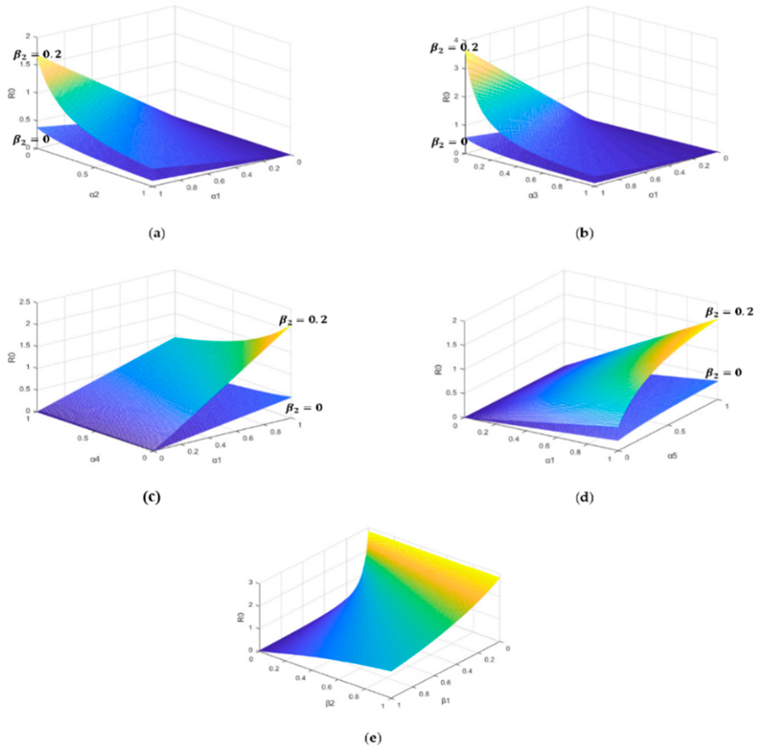
The parameters are as follows in Figure 1a: $b=0.05, {\alpha }_3=0.15, {\alpha }_4=0.3, {\alpha }_5=0.7, {\alpha }_1\in \left[0, 1\right],\mathrm{and} {\alpha }_2\in \left[0, 1\right].$ Figure 1a shows that with the increase of the diffusion rate ${\alpha }_1$, the malware is more easier prevailing. However, the self-healing rate of the infected nodes ${\alpha }_2$ has a inhibitory effect on the spread of malware. Figure 1a also shows that the charging behavior $\left({\beta }_2=0.2\right)$ makes the spread of malware easier.

(2)

The parameters are as follows in Figure 1b: $b=0.05, {\alpha }_2=0.02, {\alpha }_4=0.3, {\alpha }_5=0.7, {\alpha }_1\in \left[0, 1\right],\mathrm{and} {\alpha }_3\in \left[0, 1\right].$ Figure 1b shows that with the increase of the recovery rate of the infected nodes ${\alpha }_3$, the spread of malware can be effectively suppressed, which will provide us with the reference value in the control of malware. Similarly, Figure 1b also shows that without the charging behavior (${\beta }_2=0$), the control of malware will become easier.

(3)

The parameter settings are as follows in Figure 1c: $b=0.05, {\alpha }_2=0.02, {\alpha }_3=0.15, {\alpha }_5=0.7, {\alpha }_1\in \left[0, 1\right],\mathrm{and} {\alpha }_4\in \left[0, 1\right],$ and in Figure 1d: $b=0.05, {\alpha }_2=0.02, {\alpha }_3=0.15, {\alpha }_4=0.3, {\alpha }_1\in \left[0, 1\right],\mathrm{and} {\alpha }_5\in \left[0, 1\right].$ It is shown that the increase of the immune prevention rate ${\alpha }_4$ can suppress the spread of malware but the increase of the immune failure rate ${\alpha }_5$ helps the malware to spread.

(4)

Figure 1a–d together reflect that the charging behavior $\left({\beta }_2=0.2\right)$ will encourage the spread of malware, which will provide us with the data reference for the control of the malware spread in the SIRS-L model.

Next, the influence on the malware spread under different low-energy-node conversion rate ${\beta }_1$ and charging success rate ${\beta }_2$ are also discussed.

(5)

The parameter settings are as follows in Figure 1e: $b=0.05, {\alpha }_1=0.87,{\alpha }_2=0.02, {\alpha }_3=0.15, {\alpha }_4=0.3, {\alpha }_5=0.7, {\beta }_1\in \left[0, 1\right],\mathrm{and} {\beta }_2\in \left[0, 1\right]$. Figure 1e reflects the influence of the low-energy node conversion rate ${\beta }_1$ and the charging success rate ${\beta }_2$ on malware propagation. It is shown that if the low-energy node conversion rate ${\beta }_1$ is less than 0.2, the increase of the charging success rate ${\beta }_2$ can easily lead to the prevalence of malware. On the other side, if the low-energy node conversion rate ${\beta }_1$ is larger than 0.4, we can appropriately reduce the charging success rate ${\beta }_2$ to suppress the spread of malware.

5.2. Analysis and Display of Equilibrium Solutions

In this section, the distribution of nodes’ states under different parameters of $R_0$ and $\tau$ are discussed to verify the stability of the system and to discuss the bifurcation.

(1)

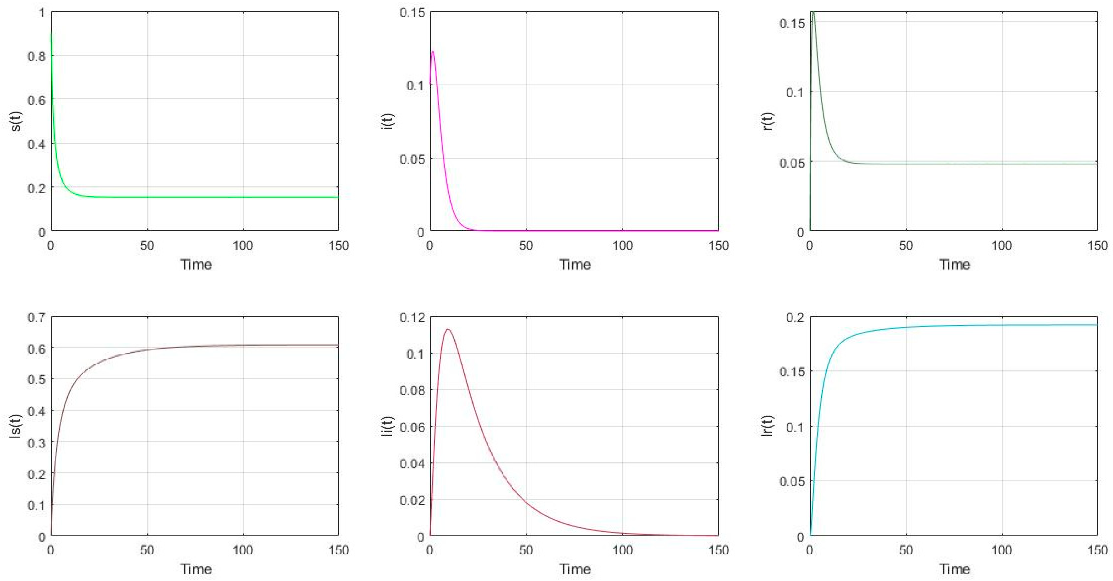
The parameter settings are as follows in Figure 2: $$\begin{gathered} b=0.05,{\alpha }_1=0.87,{\alpha }_2=0.02,{\alpha }_3=0.15,{\alpha }_4=0.3,{\alpha }_5=0.7,{\beta }_1=0.2,{\beta }_2=0, \\ and{R}_0=0.3149,\tau =0 \end{gathered}$$ with the initial value of nodes’ scale: (s(0), i(0), r(0), ls(0), li(0), lr(0))= (0.9, 0.1, 0, 0, 0, 0). It is shown that (s(∞), i(∞), r(∞), ls(∞), li(∞), lr(∞)) = (0.1520, 0, 0.0480, 0.6079, 0, 0.1920). It is shown that if the malware appears in the model (2), it will gradually disappear if $R_0<1$. It also can be shown that if ${\beta }_2=0$, the total proportion of the low-energy nodes (ls, li, lr) is larger than that of the general nodes (s, i, r).

(2)

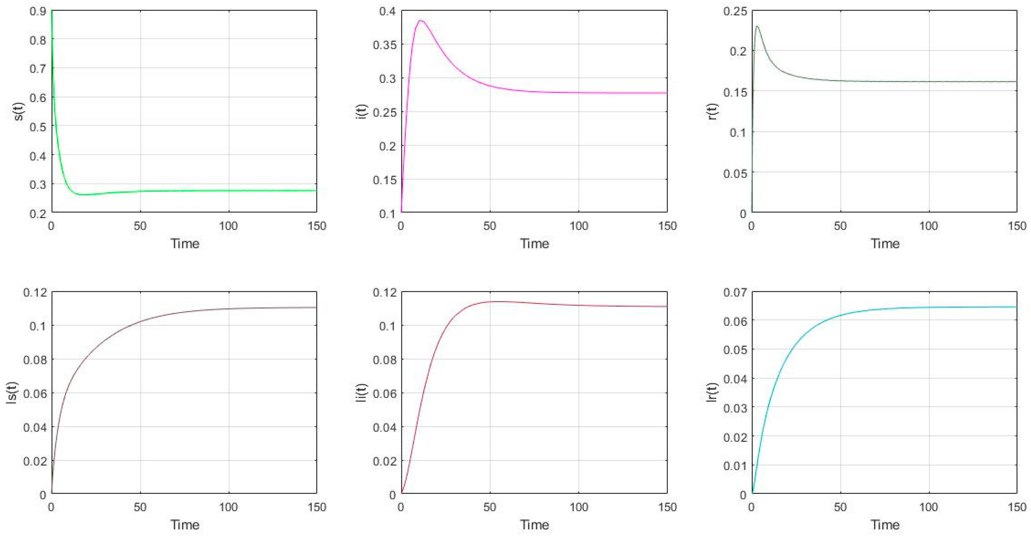
The parameter settings are as follows in Figure 3: $$\begin{gathered} b=0.05,{\alpha }_1=0.87,{\alpha }_2=0.02,{\alpha }_3=0.15,{\alpha }_4=0.3,{\alpha }_5=0.7,{\beta }_1=0.02,{\beta }_2=0, \\ and{R}_0=1.8633,\tau =0 \end{gathered}$$, with the initial value of nodes’ scale: (s(0), i(0), r(0), ls(0), li(0), lr(0))= (0.9, 0.1, 0, 0, 0, 0). It is shown that (s(∞), i(∞), r(∞), ls(∞), li(∞), lr(∞)) = (0.2756, 0.2770, 0.1616, 0.1103, 0.1109, 0.0646). It shows that the malware will prevail if $R_0>1$.

(3)

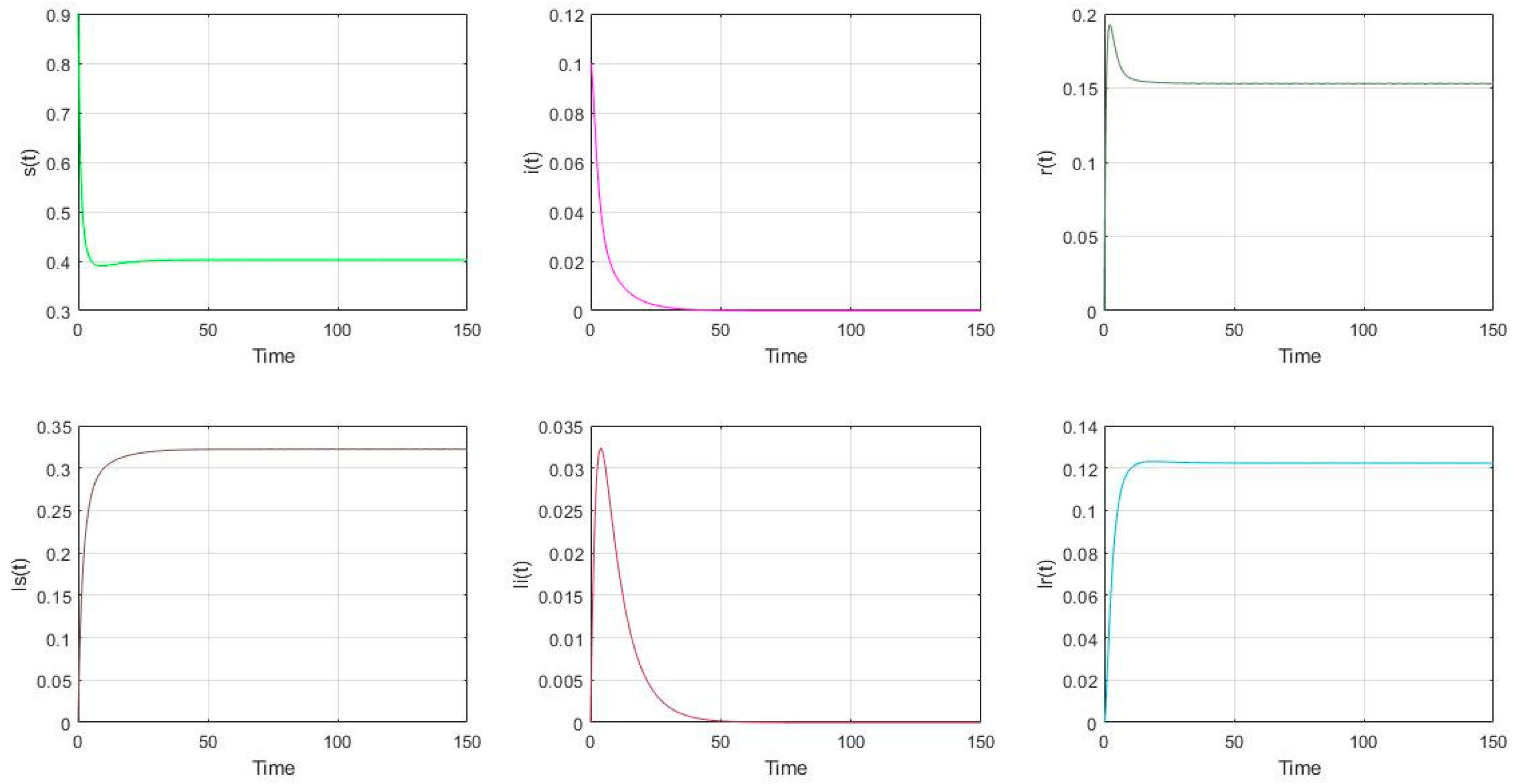
The parameter settings are as follows in Figure 4: $$\begin{gathered} b=0.05,{\alpha }_1=0.87,{\alpha }_2=0.02,{\alpha }_3=0.15,{\alpha }_4=0.3,{\alpha }_5=0.7,{\beta }_1=0.2,{\beta }_2=0.2, \\ and{R}_0=0.5743,\tau =0 \end{gathered}$$, with the initial value of nodes’ scale: (s(0), i(0), r(0), ls(0), li(0), lr(0))= (0.9, 0.1, 0, 0, 0, 0). It is shown that (s(∞), i(∞), r(∞), ls(∞), li(∞), lr(∞)) = (0.4027, 0, 0.1529, 0.3221, 0, 0.1223). It shows that if the malware appears in the model (2), it will gradually disappear if $R_0<1$. It also can be shown that if ${\beta }_2=0.2$, the total proportion of the low-energy nodes (ls, li, lr) is smaller than the proportion of the low-energy nodes in Figure 2 if the charging operation is not performed ${\beta }_2=0$.

(4)

The parameter settings are as follows in Figure 5: $$\begin{gathered} b=0.05,{\alpha }_1=0.87,{\alpha }_2=0.02,{\alpha }_3=0.15,{\alpha }_4=0.3,{\alpha }_5=0.7,{\beta }_1=0.2,{\beta }_2=0.2, \\ and{R}_0=1.3473,\tau =0 \end{gathered}$$, with the initial value of nodes’ scale: (s(0), i(0), r(0), ls(0), li(0), lr(0)) = (0.9, 0.1, 0, 0, 0, 0). It is shown that (s(∞), i(∞), r(∞), ls(∞), li(∞), lr(∞)) = (0.2988, 0.1204, 0.1364, 0.2391, 0.0963, 0.1091). It shows that the malware will prevail if $R_0>1$. Similarly, it also can be shown that if ${\beta }_2=0.2$, the total proportion of the low-energy nodes (ls, li, lr) is smaller than the proportion of the low-energy nodes in Figure 2 if the charging operation is not performed ${\beta }_2=0$. The total proportion of the low-energy nodes is similar to the corresponding proportion in Figure 4, which represents the proportion of low-energy nodes is only related to ${\beta }_1$ and ${\beta }_2$.

The above results (1)–(4) can be summarized as follows: the system is locally stable on the premise that the parameters meet the hypothesis (H1). In addition, if $R_0\ge 1$, the malicious software will persist in the system, while if $R_0<1$, the malicious software will be finally cleared. Next, we verify the bifurcation of the system.

(5)

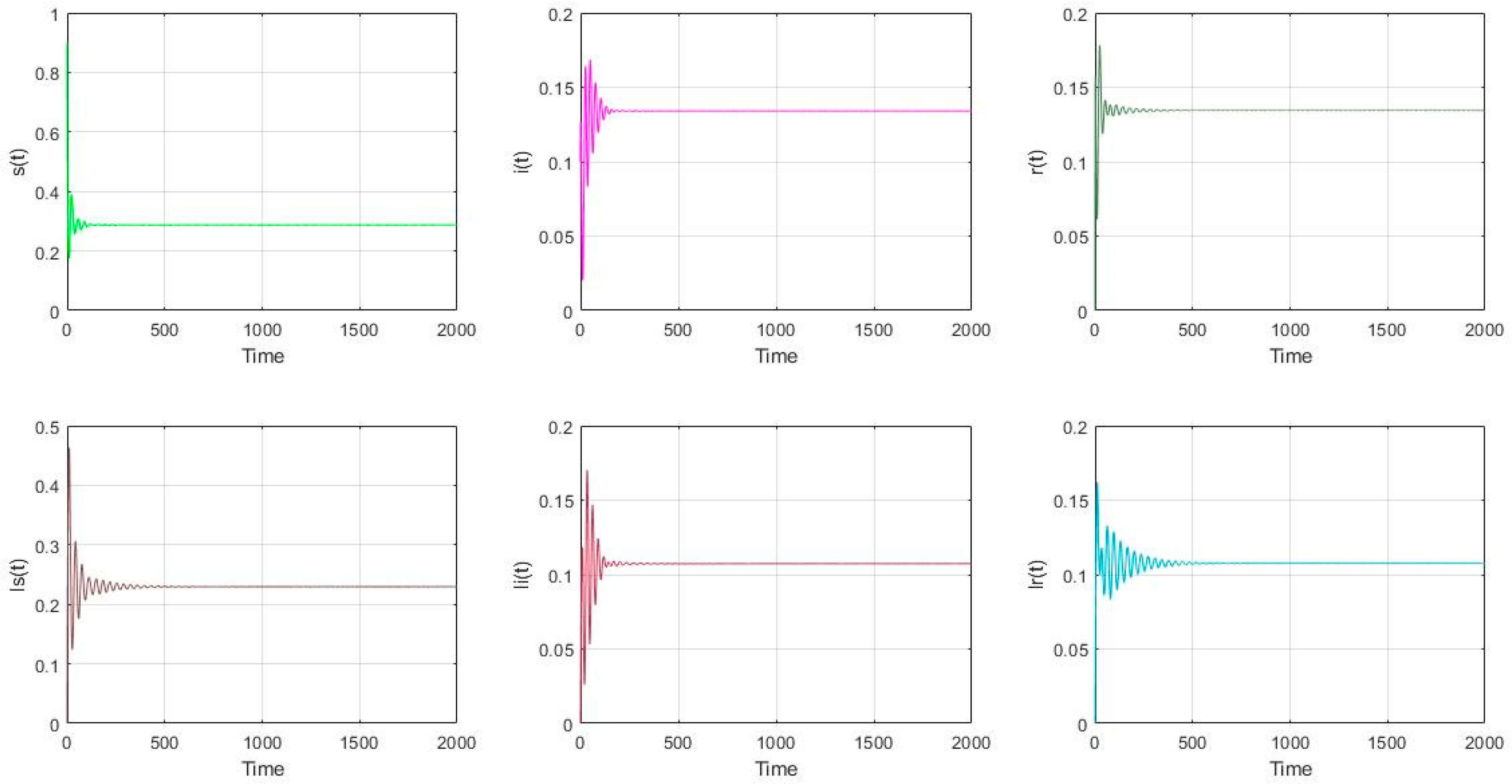
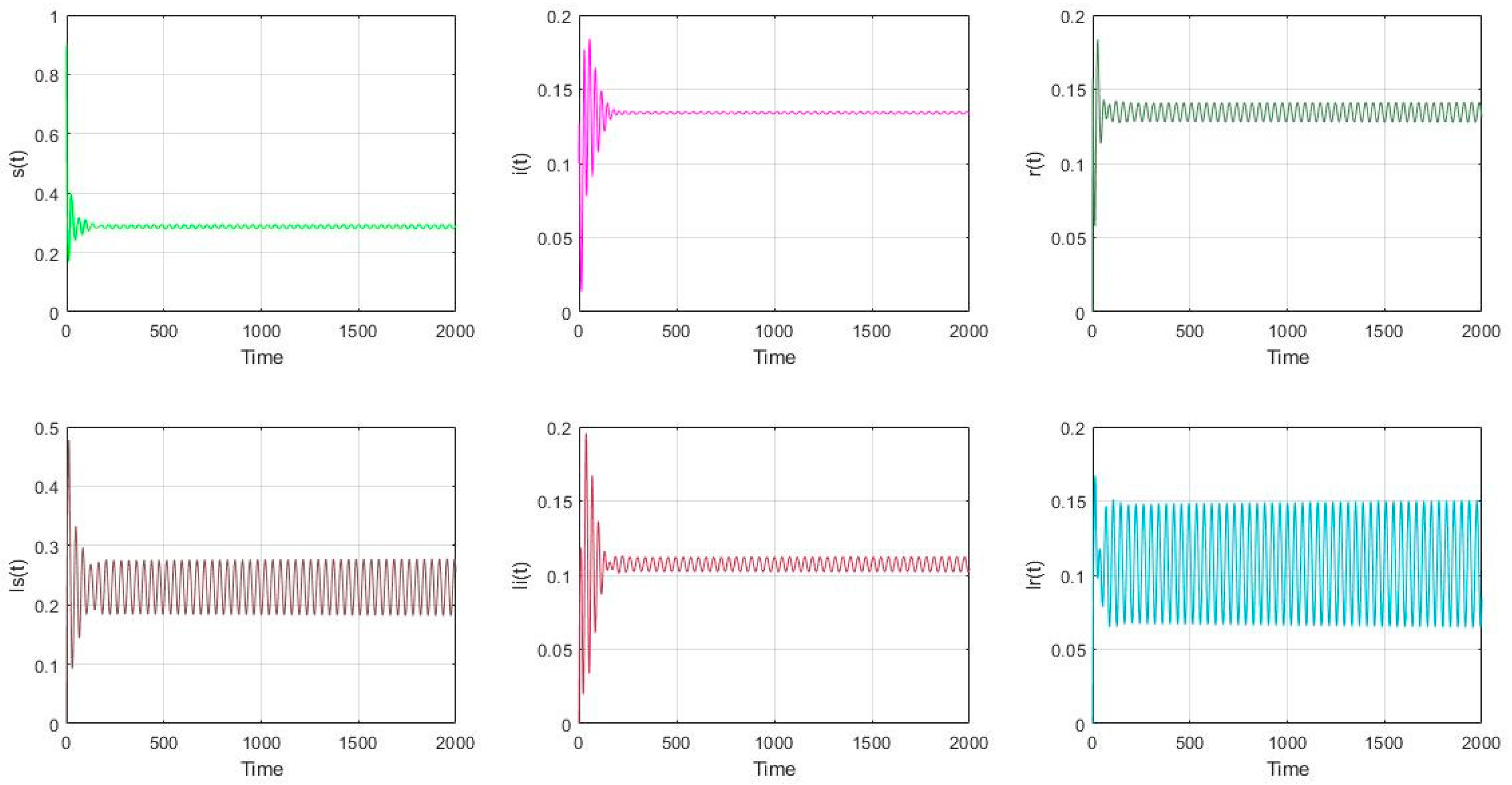
The parameter settings are as follows in Figure 6 and Figure 7: $$\begin{gathered} b=0.05,{\alpha }_1=0.9059,{\alpha }_2=0.02,{\alpha }_3=0.15,{\alpha }_4=0.3,{\alpha }_5=0.7,{\beta }_1=0.2,{\beta }_2=0.2, \\ and{R}_0=1.4029 \end{gathered}$$, with the initial value of nodes’ scale: (s(0), i(0), r(0), ls(0), li(0), lr(0)) = (0.9, 0.1, 0, 0, 0, 0). It can be calculated that ${\tau }_0=11.5370$ and ${\omega }_0=0.2254$. In Figure 6, it can be seen that the model (2) is asymptotically stable if $\tau =10.25<{\tau }_0=11.5370$. What’s more, in Figure 7, the model (2) undergoes a Hopf bifurcation if $\tau =11.74>{\tau }_0=11.5370$. According to Equation (41) and Theorem 2, the following parameters can be obtained: $$\begin{gathered} {\lambda }^{\prime }\left({\tau }_0\right)=0.0292+0.0328i,C_1\left(0\right)=-1.4520+0.7622i,{\mu }_2=49.7260>0, \\ {\beta }_2^{*}=-2.9040<0,\mathrm{and}{T}_2=-0.9203<0. \end{gathered}$$ The result can be concluded that the Hopf bifurcation is supercritical, the bifurcating periodic solutions are stable and the period of the periodic solutions decreases.

6. Conclusions

This article puts forward a novel SISR-L model that considers the low-energy status nodes. Combined with the reality, the charging delay $\tau$ is introduced in the model to study the bifurcation. We have proved that the system is locally stable under certain conditions. In addition, the influence of different parameters on the spread of malware is displayed in the simulation. It is worth noting that in the SISR-L system, the charging behavior will make it more difficult to control the spread of malware. On the analysis of bifurcation, we reveal that the SISR-L model is locally asymptotically stable if the charging delay is less than ${\tau }_0$, and the model undergoes a Hopf bifurcation at the endemic solution $e_{+}$ if the charging delay is larger than ${\tau }_0$. Finally, the properties of Hopf bifurcation were explored through applying the normal form method and the center manifold theorem. All the analyses can provide theoretical reference for the control of malware propagation in the SISR-L model.

References

- Rashid, B.; Rehmani, M.H. Applications of wireless sensor networks for urban areas: A survey. J. Netw. Comput. 2016, 60, 192–219. [Google Scholar] [CrossRef]
- Oliviero, F.; Romano, S.P. A reputation-based metric for secure routing in wireless mesh networks. In Proceedings of the IEEE GLOBECOM 2008–2008 IEEE Global Telecommunications Conference, New Orleans, LA, USA, 30 November–4 December 2008; pp. 1–5. [Google Scholar]
- Rehman, A.U.; Rehman, S.U.; Raheem, H. Sinkhole attacks in wireless sensor networks: A survey. Wirel. Pers. Commun. 2019, 106, 2291–2313. [Google Scholar] [CrossRef]
- Alajmi, N. Wireless sensor networks attacks and solutions. arXiv 2014, arXiv:1407.6290. [Google Scholar]
- Ngai, E.C.; Liu, J.; Lyu, M.R. On the intruder detection for sinkhole attack in wireless sensor networks. In Proceedings of the 2006 IEEE International Conference on Communications, Istanbul, Turkey, 11–15 June 2006; Volume 8, pp. 3383–3389. [Google Scholar]
- Hu, Y.C.; Perrig, A.; Johnson, D.B. Packet leashes: A defense against wormhole attacks in wireless networks. In Proceedings of the IEEE INFOCOM 2003. Twenty-second Annual Joint Conference of the IEEE Computer and Communications Societies (IEEE Cat. No. 03CH37428), San Francisco, CA, USA, 30 March–3 April 2003; Volume 3, pp. 1976–1986. [Google Scholar]
- Yu, B.; Xiao, B. Detecting selective forwarding attacks in wireless sensor networks. In Proceedings of the 20th IEEE International Parallel & Distributed Processing Symposium, Rhodes Island, Greece, 25–29 April 2006; p. 8. [Google Scholar]
- Salehi, S.A.; Razzaque, M.A.; Naraei, P.; Farrokhtala, A. Detection of sinkhole attack in wireless sensor networks. In Proceedings of the 2013 IEEE International Conference on Space Science and Communication (IconSpace), Melaka, Malaysia, 1–3 July 2013; pp. 361–365. [Google Scholar]
- Sundararajan, R.K.; Arumugam, U. Intrusion detection algorithm for mitigating sinkhole attack on LEACH protocol in wireless sensor networks. J. Sens. 2015, 2015. [Google Scholar] [CrossRef] [Green Version]
- Chen, C.; Song, M.; Hsieh, G. Intrusion detection of sinkhole attacks in large-scale wireless sensor networks. In Proceedings of the 2010 IEEE International Conference on Wireless Communications, Networking and Information Security, Beijing, China, 25–27 June 2010; pp. 711–716. [Google Scholar]
- Liang, C.J.M.; Musăloiu-e, R.; Terzis, A. Typhoon: A Reliable Data Dissemination Protocol for Wireless Sensor Networks. In European Conference on Wireless Sensor Networks; Springer: Berlin/Heidelberg, Germany, 2008; pp. 268–285. [Google Scholar]
- Song, Y.; Jiang, G.P. Model and Dynamic Behavior of Malware Propagation over Wireless Sensor Networks. In International Conference on Complex Sciences; Springer: Berlin/Heidelberg, Germany, 2009; pp. 487–502. [Google Scholar]
- Yetgin, H.; Cheung, K.T.K.; El-Hajjar, M.; Hanzo, L.H. A Survey of Network Lifetime Maximization Techniques in Wireless Sensor Networks. IEEE Commun. Surv. Tutor. 2017, 19, 828–854. [Google Scholar] [CrossRef] [Green Version]
- Rasheed, A.; Mahapatra, R.N. The Three-Tier Security Scheme in Wireless Sensor Networks with Mobile Sinks. IEEE Trans. Parallel Distrib. Syst. 2010, 23, 958–965. [Google Scholar] [CrossRef]
- Lin, C.; Shang, Z.; Du, W.; Ren, J.K.; Wang, L.; Wu, G.W. CoDoC: A Novel Attack for Wireless Rechargeable Sensor Networks through Denial of Charge. In Proceedings of the IEEE INFOCOM, Paris, France, 29 April–2 May 2019. [Google Scholar]
- Desmedt, Y.; Frankel, Y. Shared generation of authenticators and signatures. In Annual International Cryptology Conference; Springer: Berlin/Heidelberg, Germany, 1991; pp. 457–469. [Google Scholar]
- Weidong, C.; Dengguo, F. A group of threshold group-signature schemes with privilege subsets. In Progress on Cryptography; Springer: Boston, MA, USA, 2004; pp. 81–88. [Google Scholar]
- Yi, S.; Dengguo, F. The Design and analysis of a new group of (tj, t, n) threshold group signature scheme. China Crypto. 2000. Available online: https://en.cnki.com.cn/Article_en/CJFDTotal-ZKYB200102002.htm (accessed on 20 July 2021).
- Wang, X.; Dong, Y. Threshold group signature scheme with privilege subjects based on ECC. In Proceedings of the 2010 International Conference on Communications and Intelligence Information Security, Nanning, China, 13–14 October 2010; pp. 84–87. [Google Scholar]
- Tanachaiwiwat, S.; Helmy, A. Encounter-based worms: Analysis and defense. Ad Hoc Netw. 2009, 7, 1414–1430. [Google Scholar] [CrossRef] [Green Version]
- Khayam, S.A.; Radha, H. Using signal processing techniques to model worm propagation over wireless sensor networks. IEEE Signal Process. Mag. 2006, 23, 164–169. [Google Scholar] [CrossRef]
- Batista, F.K.; Martin del Rey, A.; Queiruga-Dios, A. A new individual-based model to simulate malware propagation in wireless sensor networks. Mathematics 2020, 8, 410. [Google Scholar] [CrossRef] [Green Version]
- Zhang, Z.; Si, F. Dynamics of a delayed SEIRS-V model on the transmission of worms in a wireless sensor network. Adv. Differ. Equ. 2014, 2014, 1–15. [Google Scholar] [CrossRef] [Green Version]
- Zhang, Z.; Wang, Y. Bifurcation Analysis for an SEIRS-V Model with Delays on the Transmission of Worms in a Wireless Sensor Network. Math. Probl. Eng. 2017, 2017. [Google Scholar] [CrossRef] [Green Version]
- Liu, G.; Peng, B.; Zhong, X. A Novel Epidemic Model for Wireless Rechargeable Sensor Network Security. Sensors 2021, 21, 123. [Google Scholar] [CrossRef]
- Liu, G.; Peng, B.; Zhong, X. Epidemic Analysis of Wireless Rechargeable Sensor Networks Based on an Attack–Defense Game Model. Sensors 2021, 21, 594. [Google Scholar] [CrossRef]
- Liu, G.; Peng, B.; Zhong, X.; Cheng, L.; Li, Z. Attack-Defense Game between Malicious Programs and Energy-Harvesting Wireless Sensor Networks Based on Epidemic Modeling. Complexity 2020, 2020, 1–19. [Google Scholar] [CrossRef]
- Liu, G.; Peng, B.; Zhong, X.; Lan, X. Differential Games of Rechargeable Wireless Sensor Networks against Malicious Programs Based on SILRD Propagation Model. Complexity 2020, 2020, 13. [Google Scholar] [CrossRef]
- Liu, G.; Li, J.; Liang, Z.; Peng, Z. Analysis of Time-Delay Epidemic Model in Rechargeable Wireless Sensor Networks. Mathematics 2021, 9, 978. [Google Scholar] [CrossRef]
- Liu, G.; Peng, Z.; Liang, Z.; Li, J.; Cheng, L. Dynamics Analysis of a Wireless Rechargeable Sensor Network for Virus Mutation Spreading. Entropy 2021, 23, 572. [Google Scholar] [CrossRef]
- Liu, G.; Huang, Z.; Wu, X.; Liang, Z.; Hong, F.; Su, X. Modelling and Analysis of the Epidemic Model under Pulse Charging in Wireless Rechargeable Sensor Networks. Entropy 2021, 23, 927. [Google Scholar] [CrossRef]
- Liu, G.; Shu, C.; Liang, Z.; Peng, B.; Cheng, L. A Modified Sparrow Search Algorithm with Application in 3d Route Planning for UAV. Sensors 2021, 21, 1224. [Google Scholar] [CrossRef]
- Zhu, L.; Guan, G. Dynamical Analysis of a Rumor Spreading Model with Self-Discrimination and Time Delay in Complex Networks. Phys. A Stat. Mech. Appl. 2019, 533, 121953. [Google Scholar] [CrossRef]
- Diekmann, O.; Heesterbeek, H.; Britton, T. Mathematical Tools for Understanding Infectious Disease Dynamics; Princeton University Press: Princeton, NJ, USA, 2012; Volume 7. [Google Scholar]
- Cooke, K.L.; Van Den Driessche, P. On zeroes of some transcendental equations. Funkc. Ekvacioj 1986, 29, 77–90. [Google Scholar]
- Hassard, B.D.; Kazarinoff, N.D.; Wan, Y.H.; Wan, Y.W. Theory and Applications of Hopf Bifurcation; CUP Archive: Cambridge, UK, 1981; Volume 41. [Google Scholar]