A Proposal for the Optimisation of Algorithms for the Calculation of the Energy Demands of Residential Housing

Abstract

In response to increased energy consumption and CO₂ emissions, various energy efficiency policies, standards and housing certifications have emerged around the world. These aim to measure and quantify energy efficiency and endorse homes for meeting certain standards according to consistent categories that vary by continent or country. These energy rating systems correspond to a series of criteria and formulations that, through the calculation and combination of multiple variables, establish the classification values. In Chile, there is the Energy Rating System for Housing (CEV), which performs energy efficiency calculations using dynamic heat balance spreadsheets in Microsoft^® Excel. When applied for everyday use and at a large scale, this system has the disadvantage of requiring a great deal of processing time for each simulation. This research proposes an improvement to the CEV energy demand calculation mechanism by generating a solution that takes advantage of the use of multiprocessors and implements the various algorithms in the C programming language. The results show that the CEV values obtained with the proposed calculation engine are equal to those of the current system but demonstrate a 76.5% improvement in their processing time.

1. Introduction

The construction sector is responsible for more than 36% of all energy consumption, and contributes to 39% of global carbon dioxide emissions, with a 30% increase in building energy demands expected by 2060 if systems to improve efficiency are not implemented [1]. As housing is responsible for a third of the energy consumed globally, focusing on the optimisation of energy consumption in housing is the key to reducing these figures [2]. By 2030, 80% of Europe’s population is expected to be using existing housing (i.e., less construction and more renovation); this implies an increase in energy consumption, both due to the deterioration of the infrastructure over time and the costs of the improvements to be made [3].

In light of these challenges, various housing energy policies have been created around the world [4]. These aim to reduce energy consumption and CO₂ emissions without affecting the comfort of their inhabitants through efficient architectural design and the incorporation of construction elements that optimise energy performance [5]. Energy performance certificates for dwellings have been created to standardise the assessments of such buildings. These classify dwellings based on various indicators and standardised categories to support their attributes.

In the European Union (EU), policy initiatives such as the Energy Performance of Buildings Directives (EPBDs) have encouraged the use of Energy Performance Certificates (EPCs) for the modelling and assessment of dwellings’ energy performance in response to climate change issues [6,7]. Leadership in Energy and Environmental Design (LEED) and the Building Research Establishment Environmental Assessment Method (BREEAM) are widely used in the green certification of housing and other buildings in the EU [8]. In South Korea, the use of the Green Standard for Energy and Environmental Design (G-SEED)-certified housing has increased considerably, and the government provides incentives for the purchase of G-SEED-certified housing [9]. In the United States, factors associated with public policies, market behaviour and the characteristics and costs of the energy industry influence increases in the number of energy certifications [10].

Studies show that houses with better energy ratings have higher market prices, which incentivise real estate companies to promote energy certifications in their projects [11,12,13,14]. These incentives for improved certifications encourage innovation in construction methods and the use of architectural elements for thermal balance, which has direct implications for the environmental factors they seek to impact (mainly CO₂ reduction) [15].

In the Latin American context, Brazil has been a pioneer in the incorporation of energy certification schemes. Although the Energy Efficiency Rating Technical Quality Regulations for Commercial, Service and Public Buildings (RTQ-C) have achieved significant reductions in energy consumption, there are still challenges associated with their calculation methodology, scope and implementation [16]. In Chile, private initiatives have promoted LEED, PassivHaus and DGNB certifications, but they have not been implemented at a large scale due to their costs [17]. Various proposals have emerged that seek to incorporate the characteristics of housing in Chile and the country’s specific contexts [18,19].

By 2013, the Chilean government had created the Housing Energy Rating System (SCEV), which aims to reduce emissions in new homes by 40%, and in existing homes by 20% [20]. The SCEV evaluates a home’s energy efficiency through an energy efficiency report (EER) and an energy efficiency label (EEL). These results are obtained based on the analysis of the thermal transmittance parameters of the housing envelope, its orientation and the performance of heating and cooling equipment [21].

The Chilean government has implemented dynamic heat balance spreadsheets (PBTD) using Microsoft^® Excel to facilitate the calculation of the parameters associated with the Housing Energy Rating (CEV) [22]. These spreadsheets are simple to use for single-family homes, but become more complex for large projects such as buildings or large housing complexes. Moreover, with the increase in policies encouraging housing energy certification, there is also increased demand for these evaluations. As such, the processing of large amounts of data from multiple projects is not efficient. In this context, this research proposes and implements a new mechanism for the calculation of CEV energy demands using multiprocessors and algorithms written in the C programming language. The variables and their formulations were studied and implemented in order to analyse the efficiency of the generated processes.

In order to achieve the research objectives, the research method is organised into two stages: (1) study of the problem and (2) solution’s development. Figure 1 shows a diagram of the research methodology. In the first stage, a literature review was carried out to identify the context and general aspects of housing energy certifications. The Chilean system was reviewed, and the main characteristics and challenges of the country’s CEV system were identified. Against this background, the problem to be optimised was defined: the optimisation of the CEV system’s Energy Demand Calculation Engine. In the second stage, the algorithms were developed and run for the Energy Demand Calculation Engine. The results obtained were compared with the traditional CEV system according to three metrics: (1) processing time, (2) the use of computational resources (RAM), and (3) the precision of the calculations.

2. Study of the Problem

2.1. Background and Context

Presently, Chile’s Ministry of Housing and Urban Development (MINVU), through its Technical Division of Study and Housing Development (DITEC), aims to improve people’s quality of life by designing, planning and building better cities, neighbourhoods and housing. In this context, the MINVU created the Energy Rating of Homes programme, which makes it possible to determine a dwelling’s energy consumption, enabling the institution to identify the most and least energy-efficient buildings. This programme allows the energy classification of a building to be calculated using certain pieces of architectural information. This classification is a theoretical calculation performed using a mathematical model of the building’s estimated energy demands with regard to heating, cooling, domestic hot water and lighting. It is delivered through a CEV accreditation certificate and its respective energy efficiency label. The Energy Rating of Homes makes it possible to know the delivered energy quality of a house or apartment, facilitating the search for the best project and negotiations with managers and end users [20,21].

The Spanish context in the area of certifications and energy efficiency is interesting for Chile because Chile has adopted several of Spain’s policies for the development of local standards as references. In Spain, three software programs are associated with energy certification: CE3X, LIDER and CALENER [17]. CE3X is a piece of software developed by Efinovatic and the Spanish National Centre for Renewable Energy (CENER) [23]. This program makes it possible to certify any type of building in a simplified way by obtaining any qualification, from A (the most optimal) to G (the least optimal), just as in the Chilean system. This can be adapted to the great variety of situations that the certifying technician must face, offering different options for entering the building’s data. In this way, both the thermal envelope and the installations can be entered using known, estimated and default values. CE3X was developed in Python, and it allows data entry, the calculation of values and the delivery of results. Unlike the templates used in the Chilean system, CE3X offers suggestions for possible improvements to the home that can improve its energy rating. It also has a friendly, intuitive and easy-to-use user interface. The main features of this software are as follows:

• It uses hybrid procedures based on energy simulations corrected with real data and measurements.
• It assigns importance to the proposal of measures to improve energy efficiency.
• It was designed such that, depending on the improvement measures pursued, the necessary initial data are adapted, simplifying the energy consumption calculation process.
• The procedures were developed so as to make maximum use of the information obtained through inspections and reviews.

One of CE3X’s shortcomings is that it only performs the calculations once, without adding the housing rotation variable to simulate the climate in different directions. In spite of this, the program is a simplified option compared with other systems, as it is based on the indirect control of a home’s energy demands by the limitation of the characteristic parameters of the enclosures and interior partitions that make up its thermal envelope. The verification is performed by comparing the values obtained in the calculation with the limit values allowed by the Spanish standards [24].

The LIDER and CALENER programs offer a more general option based on the evaluation of buildings’ energy demands by means of comparison with a reference building. LIDER enables the calculation of the limitations of the energy demand, but its use is restricted to buildings with no more than 100 different spaces (e.g., rooms) and no more than 500 enclosures of the building envelope. CALENER allows for the calculation of a building’s energy rating. It offers two versions: (1) CALENER VyP for residential buildings and small tertiary-sector buildings, and (2) CALENER GT for large tertiary-sector buildings [23]. There is also a tool that joins both programs, called the Unified Tool LIDER/CALENER (HULC), which issues a report for the Energy Certification of Buildings in PDF and XML formats along with the necessary information for registration.

Table 1. Comparison table of the housing energy rating systems.

Characteristic	Templates (MINVU)	CE3X	LIDER CALENER
Generates housing energy rating	✓	✓	✓
Intuitive and easy-to-use user interface	×	✓	✓
Housing rotation	✓	×	✓
Suggests possible improvements	×	✓	✓
Outputs data in optimal format for recording	×	✓	✓
Fast calculation	×	✓	✓
3D visualisations of houses	×	×	✓
Evaluation of projects at a massive scale	✓	×	×
Precision of calculations	✓	✓	✓
Processing time	×	✓	✓
Use of computational resources	×	×	✓
Usability and user experience	×	✓	✓

shows a comparison of the Chilean energy efficiency calculation system with its Spanish counterparts. This comparison indicates that the Chilean system has only four of the 12 relevant characteristics identified for these systems.

As shown in Table 1, the calculation system that uses processing templates is highly deficient compared with the other existing tools in this area. This can mainly be seen in the last three criteria compared, which are directly related to the calculations and processing itself. After reviewing and considering this preliminary background in depth, a test was carried out to analyse one of the critical points, namely the processing time or runtime. A set of test data was executed on three different pieces of computer equipment: one local machine belonging to a member of this research team and two external servers in service-on-demand mode, one from Google Compute Engine and the other from the IBM Cloud. These tests were performed to analyse whether the computational resources directly affected the high runtime registered locally. For this preliminary test, 30 different dwelling cases were executed in each team. The average runtimes for each facility are presented in

Table 2. Comparative results of the preliminary testing process.

Equipment/Service	Characteristics	Average Runtime/Case
Research Team Computer	Intel Core i7/4 GB RAM	22′54″
Google Compute Engine	Intel Xeon 2.8 GHz/32 GB RAM	21′53″
IBM Cloud	Intel Xeon 2.6 GHz/60 GB RAM NVIDIA TESLA P100/16 GB VRAM	29′13″

.

The results showed that the characteristics of the computational equipment did not directly affect the processing time. Rather, the performance was affected by the efficiency of the macro code, as measured by the algorithmic complexity and arithmetic operations involved. These aspects are thus considered in the development of this work when determining housing energy demands.

2.2. Problem to Be Optimised

The CEV system, which enables the calculation of a house’s energy quality, is designed using templates programmed in the Visual Basic for Applications (VBA) interface [21]. It is organised into three PBTD, wherein energy demands and consumption are calculated: (1) PBTD, Architecture Data; (2) PBTD, the Energy Demand Calculation Engine; and (3) PBTD, Equipment and Results Data. Figure 2 visualises these steps.

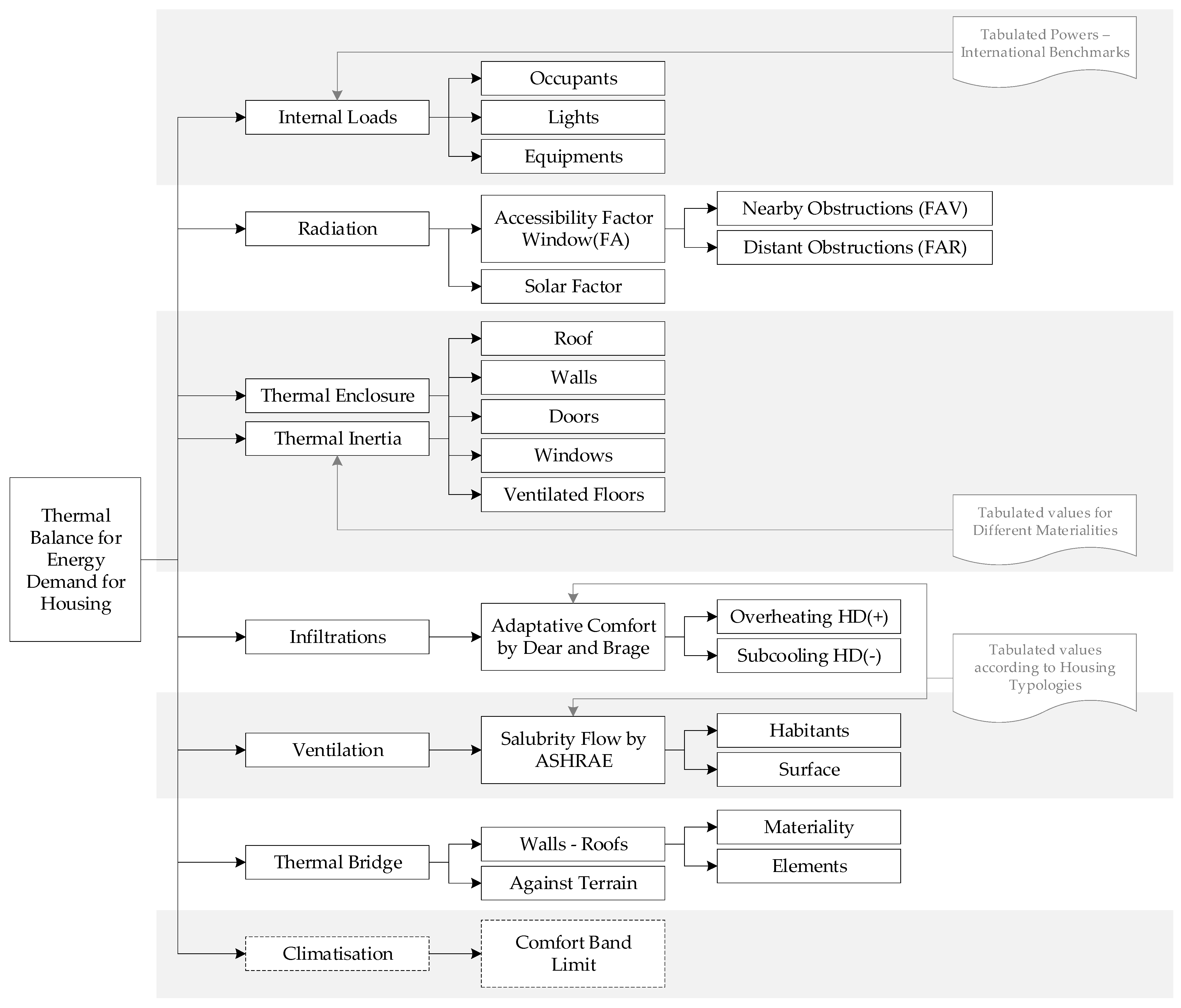
This research focuses on PBTD 2, the Energy Demand Calculation Engine. In this step of the CEV system, the calculation of the energy demand of the house is developed. This calculation is related to various internal and external factors: internal load, radiation, thermal enclosure, thermal inertia, infiltrations, ventilation, the thermal bridge and climatisation. Figure 3 schematically shows these elements in a typical house. Climatisation is an element that depends on other variables that are not considered for the purposes of this study. Therefore, the energy demand is directly influenced only by the elements of the construction, such that the temperature can vary freely.

Figure 4 provides an overview of the factors that influence the calculation of the temperature balance. All of the factors have been grouped to identify the elements related to each factor, and to clarify which elements are involved in the calculations.

The CEV system, based on the scheme in Figure 3 and the factors shown in Figure 4, calculates a house’s energy demand according to Equation (1):

$$E\left[Wh\right]={\displaystyle \sum }\left(\begin{array}{c}{\varnothing }_{internal loads}+{\varnothing }_{radiation}\pm {\varnothing }_{thermal enclosure}\pm {\varnothing }_{thermal inertia}\\ \pm {\varnothing }_{infiltrations}\pm {\varnothing }_{ventilation}\pm {\varnothing }_{thermal bridge}\pm {\varnothing }_{climatisation}\end{array}\right),$$

(1)

where:

• Internal Loads corresponds essentially to the heat and lighting used by occupants, which depend on the use of space related to power, tabulated according to international regulations.
• Radiation corresponds to the radiation that enters the system through the windows. It is affected by the orientation of the windows, possible obstructions (both near and far) and the solar factor. Of the total heat that enters in this way, 70% is absorbed by the mass of the system, which comes from the construction elements, while the remaining 30% goes directly into the air.
• Thermal Enclosure corresponds to the heat transfer related to the elements associated with the thermal enclosure, including flows through the roofs, floors, walls and windows.
• Thermal Inertia corresponds to the constructive components, which add mass to the system and allow for the exchange of heat with the interior air via convection. The values considered for this factor are tabulated for different materials.
  Infiltrations corresponds to air renewals due to tabulated infiltrations associated with different types of housing.
• Ventilation corresponds to the air renewals per hour or the ventilation rate, which are associated with different conditions of housing use.
• Thermal Bridge corresponds to the coefficients of heat transfer associated with different thermal jumpers.
• Climatisation corresponds to the heat provided by an air conditioning system—that is, the heat necessary to keep the interior temperature within the limits of the comfort band when the room temperature escapes this range.

Table 3. Housing Energy Rating (CEV) system factors and formulae.

Formula		Description/Important Facts
Technical Factor: Internal Loads
${\varnothing }_{internal}={\displaystyle {\displaystyle \sum }_{i=1}^3}{Q}_{gen\left(i\right)}=Q_{ge{n}_{{}_{Ocup}}}+Q_{ge{n}_{{}_{Ilum}}}+Q_{ge{n}_{{}_{Apli}}}$	(2)	It depends on the time of day when the thermal balance is being carried out, where t varies from 0 to 23 h.
Where: $Q_{ge{n}_{\left(1\right)}}=Q_{ge{n}_{\_Ocup}}:heat generated by Occupants$ $Q_{ge{n}_{\left(2\right)}}=Q_{ge{n}_{\_Ilum}}:heat generated by Lights$ $Q_{ge{n}_{\left(3\right)}}=Q_{ge{n}_{\_Apli}}:heat generated by Equipments$		$Ocuppants:\left\{\begin{array}{c}98.4 \left[w\right]\\ 82.0 \left[w\right]\end{array}\right\} \forall 7 h\le t\le 22 h$ $\forall 22 h\le t\le 7 h$ $Ligths:\left\{\begin{array}{c}1.5 \left[\frac{w}{m2}\right]\\ 0 \left[w\right]\end{array}\right\}$
Linear Interpolation Function (LIF), for each		$\forall 7 h\le t \le 22 h and Lux<250$
$Q_{ge{n}_{\left(i\right)}}:LIF (((Q_{gen\left(i\right)}\left[month\right]\left[hour+1\right]$ $-Q_{gen\left(i\right)}\left[month\right]\left[hour+1\right]/\Delta t)\ast sec)$ $+Q_{gen\left(i\right)}\left[month\right]\left[hour\right])\ast floor\_area)$	(3)	$\forall 22 h\le t \le 7 h and Lux\ge 250$ $Equipments:0\left[w\right]$
$\Delta t=\left(\left(hour+1\right)\ast 3600\right)-\left(hour\ast 3600\right)$	(4)	(Values according to international data, NCH 3309)
Technical Factor: Radiation
$\varnothing Rad={\displaystyle \sum }\varnothing solar\ast FSi\ast Ai\ast FAVi\ast FARi$	(5)	Radiation is calculated for each of the 8 vertical directions; North, North East, East, South East, South, South West, West and North West and the horizontal position.
$\varnothing solar:radiation flow$ $FSi:solarfactor windows$ $Ai:windows glass area$ $FAVi:Nearby Obstructions Factor$ $FARi:Distant Obstructions Factor$
Technical Factor: Thermal Enclosure (TE) and Thermal Inertia (TI)
${\varnothing }_{Real}={\varnothing }_{Thermal Enclosure}+{\varnothing }_{Thermal Inertia}$	(6)	The Thermal Enclosure is made up of all opaque and translucent elements. Each element of the Thermal Enclosure contributes a certain amount of mass to the system. The masses of each element contributes are added to generate a total accumulated mass. This mass only exchanges heat with the interior air of the house through factor: h = 8.3 [W/m2K] Thermal inertia, which corresponds to the value recommended by Chilean legislation for the interior face of walls fma: the function computes the result without losing precision in any intermediate result.
${\varnothing }_{TE}=Q_{Wall}+Q_{Window}+Q_{Roof}+Q_{Floor}$	(7)
where
${\mathrm{Q}}_{Wall}={\displaystyle {\displaystyle \sum }_{i=1}^8}wall\_estructure\left(i\right)+\left(q_{mass}\ast m_{wall}\right)$	(8)
$i:orientation on a surface$ $q_{mass}:heat of the mass$ $m_{wall}:mass participation of wall \left\{0,1\right\}$
${\mathrm{Q}}_{Window}={\displaystyle {\displaystyle \sum }_{i=1}^8}window\_estructure\left(i\right)$	(9)
${\mathrm{Q}}_{Roof}=roof\_estructure+\left(q_{mass}\ast m_{roof}\right)$	(10)
$m_{roof}:mass participation of roof$
${\mathrm{Q}}_{Floor}=q_{floo{r}_{ventilated}}+q_{floo{r}_{ground}}$ ${\mathrm{Q}}_{Floor\_ventilated}=fma\left(q_{mass}, m_{floor\_ventilated}\right)$ ${\mathrm{Q}}_{Floor\_ground}=fma\left(q_{mass}, m_{floor\_ground}\right)$	(11)
Technical Factor: Infiltrations and ventilations
$Q_{infiltrations}=volume\ast \left(\left(\frac{mont{h}_{dat{a}_{RAH}}}{3600}\right)\ast 60\left[sec\right]\right)\ast {\rho }_{AIR}\ast C_{air}\ast (\Delta T/60\left[sec\right])$	(12)	The comfort band uses the 1998 Adaptive Comfort Adaptive Comfort method proposed in Ashrae The temperature average will depend on the month and thermal zone where the house is located, and they vary during the day and night (22:00 to 7:00), with a variation where a range of 2.5 °C above or below neutral temperature is considered to an average comfort interior temperature (Tn): $T{n}_{max\left[°C\right]}=Tn+2.5$ $T{n}_{min\left[°C\right]}=Tn-2.5$ Therefore: HD(+): the number of hours that the temperature is above the comfort band are directly the hours of discomfort or also known as hours of Overheating. HD(−): the number of hours that the temperature is below the comfort band are directly the hours of discomfort or also known as hours of Subcooling.
$volume=area\ast h$ $RAH=air hour replacemen\mathrm{t}$ ${\mathsf{\rho }}_{\mathrm{AIR}}=air desity (1.2 \left[kg/m^3\right])$ ${\mathrm{C}}_{air}=specific air heat (1000\left[\frac{J}{kgK}\right])$ $\Delta \mathrm{T}=Temperatur{e}_{outdoor}-Temperatur{e}_{indoor}$
Technical Factor: Thermal bridges
$Q_{Thermal Bridge}={\displaystyle {\displaystyle \sum }_{i=1}^5}{Q}_{thermal\_bridge\left(i\right)}\ast \Psi \ast L\ast A\ast \Delta T$	(13)	Where each thermal bridge represents: (P01) a protruding corner between two walls or a wall and a roof slab. This bridge generates an increase in its surface. (P02) an incoming corner between two walls or a wall and a ventilated floor slab. This bridge generates a decrease in its surface. (P03) the encounter between a perimeter wall and an interior wall or between a perimeter wall and an interior floor. (P04) the encounters between a wall and some element that stands out from the outer perimeter lead of the walls, such as cornices or terraces. (P05) the encounter between the window frame and the wall where it is housed.
$thermal\_bridg{e}_{\left(i\right)}\dots i \left\{\mathrm{1..5}\right\}$ $L:thermal\_bridge\_length\left[m\right]$ $\Delta T^{°}=Temperatur{e}_{outdoor}-Temperatur{e}_{indoor}\left[K\right]$ $\mathsf{\Psi }:The linear coefficient of heat transfer\left[W/mK\right]$ $A:area \left[m^2\right]$

shows the Housing Energy Rating (CEV) system factors and formulae.

After calculating the parameters in Table 3, and once all of the flows have been defined, it is possible to inject (heating) or withdraw (cooling) heat from the system in order to keep the temperature within the defined comfort range.

Currently, all of the energy demand calculation processing described above is carried out using macros—programming codes that are used to automate tasks and calculations. Depending on the type and frequency of the calculations, the response times may be affected along with the resource use of the computer where they are executed. All of the aforementioned calculations are carried out every 60 s, evaluating the temperature inside the room based on the flows of the input variables.

3. Solution Development

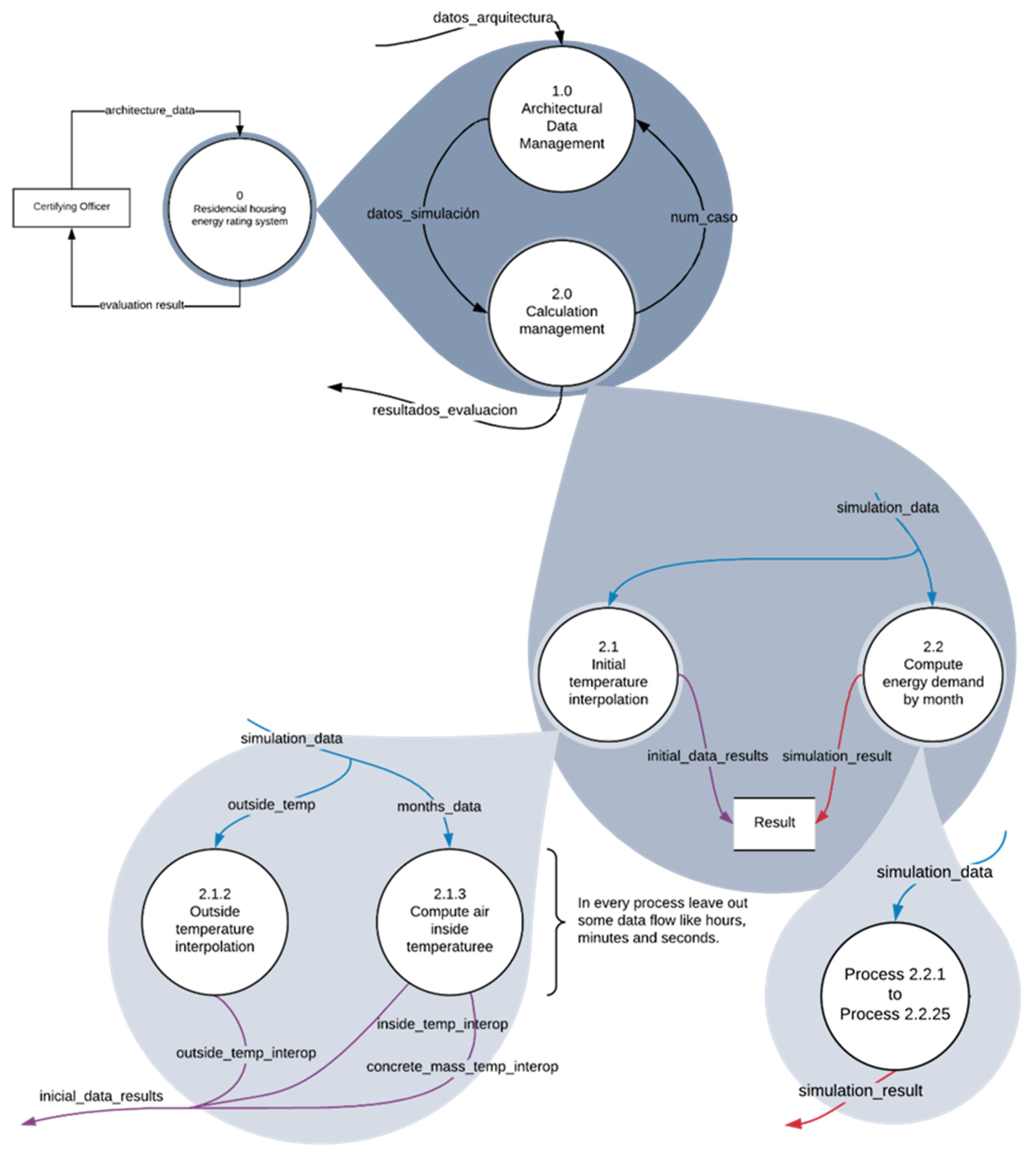
Considering the previous context, and in order to write a program using threads of execution that allow for the optimisation of the calculations involved, we needed to model the various associated processes. For the modelling of the processes involved, data flow diagrams (DFD) were used, because they are a simple and easy-to-understand notation, to represent the interaction of the interfering elements, in addition to allowing us to structure the logic of the calculations required in the development of the algorithms implemented. These are shown in Figure 5, Figure 6, Figure 7 and Figure 8 along with their corresponding algorithms. Figure 5 shows the general diagram of the programming performed. Based on the procedures of the problem studied, the development was based on the optimisation of the algorithms associated with process 2.0 (Calculation management), particularly in process 2.2 (Compute energy demand by month) and its 25 sub-processes (processes 2.2.1–2.2.25).

The algorithms presented show a general idea of the processes involved in these, and the number of lines of code implemented is extensive in order to include them completely; however, it is possible to visualize some general operations, calls to external functions and others developed to modularize the code, in addition to the use of programming in threads, which allow the development of parallel programs that scale appropriately in the environment of a machine that has several processors working simultaneously, providing a model for the handling of several transactions and calculations.

The implemented algorithms were programmed in C using threads that can make resource use more efficient and improve response times. When working with threads, a program can execute different tasks at the same time by creating a new process and simultaneously creating a new execution thread. In a computer with a single processor, the operating system can very quickly run a program’s sections in turns (by time segments), giving a sense of emulated simultaneous processors.

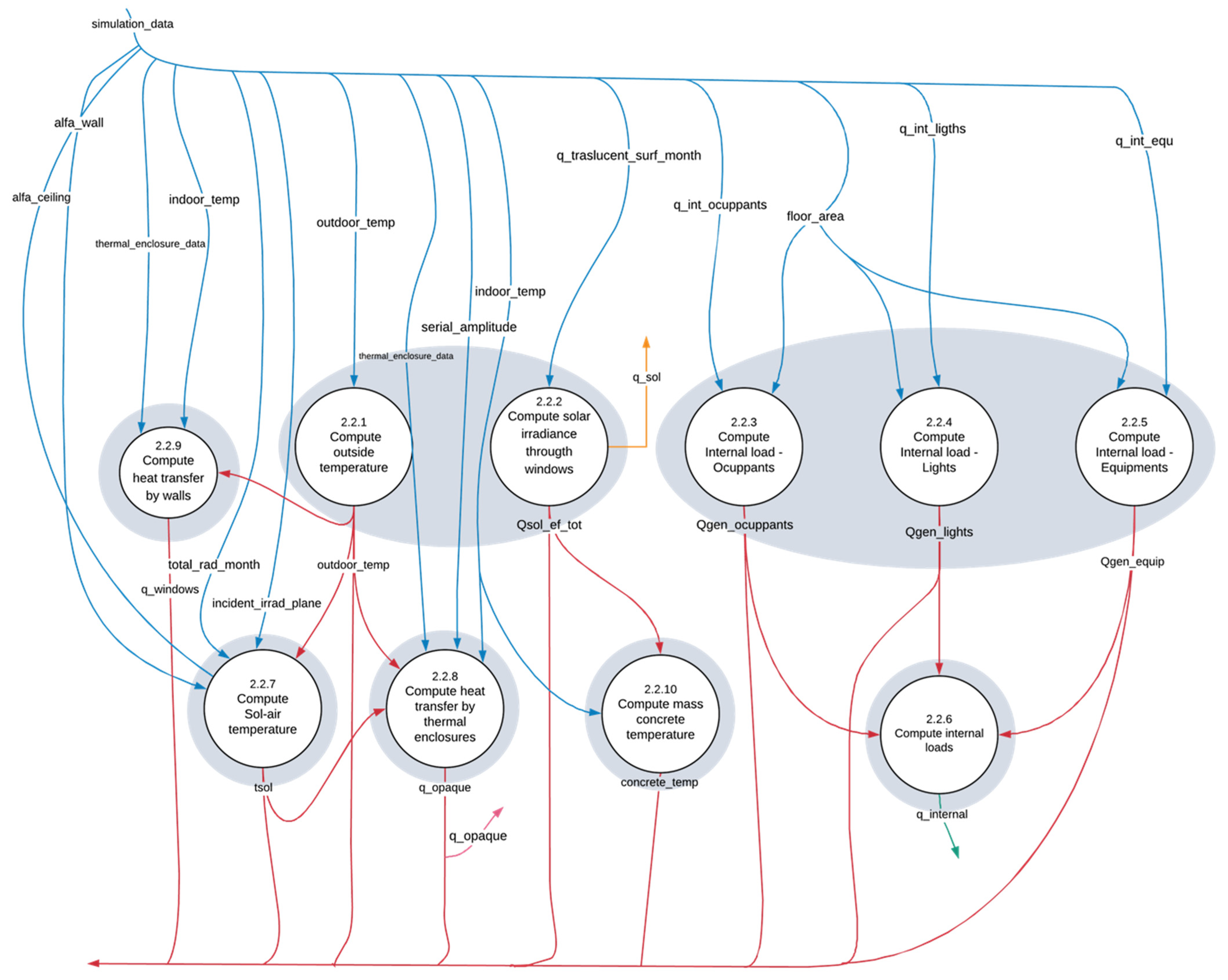
Figure 6, Figure 7 and Figure 8 detail how the different processes are connected in order to obtain the indicated parameters. Algorithms 1 through 14 show the programming of these processes. Some algorithms group more than one process together in order to facilitate the technical explanation.

Figure 6 shows the first part of the process of obtaining the energy demand solution. The blue lines represent the input data for the various processes (architectural information, weather conditions and internal loads), and the red lines show the output data of this principal process.

Algorithm 1 represents the process of obtaining the outside temperature and solar irradiance though the windows over a given period. In both procedures, linear interpolation is applied to the analysed variable based on the process in question. Process 2.2.1 corresponds to the outside temperature according to simulation time (hour and month), and process 2.2.2 is applied to solar irradiance through the windows corresponding to the simulation time.

Algorithm 1. Compute outside temperature (2.2.1) and Compute solar irradiance through windows (2.2.2)
1:	//Process 2.2.1
2:	resultado[idx_resultado].temp_ext
3:	interpolacion(temperatura_exterior[idx_mes][idx_hora + 1],
4:	temperatura_exterior[idx_mes][idx_hora],dx,idx_seg);
5:	//Process 2.2.2
6:	resultado[idx_resultado].qsol_ef_tot =
7:	interpolacion(sup_taslucida_mes[idx_mes][idx_hora + 1],
8:	sup_taslucida_mes[idx_mes][idx_hora], dx, idx_seg);
9:	//Get the previous qsol
10:	q_sol = resultado[idx_resultado − 1].qsol_ef_tot;

Algorithm 2 represents the three processes involved in computing the internal loads of a dwelling by use. This process applies a linear interpolation between the variables of use by the occupants of the dwelling, the heat input through the different lighting fixtures defined in a range of time, and the consumption of different equipment providing heat to the dwelling. Each of these variables corresponds to the simulation time.

Algorithm 2. Compute Internal load—Ocuppants (2.2.3), Compute Internal load—Lights (2.2.4) and Compute Internal load—Equipments (2.2.5)
1:	//Process 2.2.3
2:	resultado[idx_resultado].q_gen_pers = interpolacion(calor_personas[idx_mes][idx_hora + 1],
3:	calor_personas[idx_mes][idx_hora], dx, idx_seg) * area_piso
4:	//Process 2.2.4
5:	resultado[idx_resultado].q_gen_ilum = interpolacion(calor_iluminacion[idx_mes][idx_hora + 1],
6:	calor_iluminacion[idx_mes][idx_hora],dx, idx_seg) * area_piso
7:	//Process 2.2.5
8:	resultado[idx_resultado].q_gen_equip = interpolacion(calor_equipos[idx_mes][idx_hora + 1],
9:	calor_equipos[idx_mes][idx_hora],dx,idx_seg) * area_piso

Algorithm 2 obtains the data simulated in the previous processing cycle, adds them and yields the internal loads of the evaluated house (according to Algorithm 3).

Algorithm 3. Compute internal loads (2.2.6)
1:	//Add the n-1 internal loads
2:	q_internas = resultado[idx_resultado − 1].q_gen_pers + resultado
3:	[idx_resultado − 1].q_gen_ilum + resultado[idx_resultado − 1].q_gen_equip

Subsequently, the sol-air calculation is performed using Equation (14), which aims to obtain the cooling load of the different external walls of the evaluated house (according to Algorithm 4).

$$T_{sol-air}=T_0+\frac{\left(a\ast I-\Delta Q_{ir}\right)}{h_0} ,$$

(14)

where:

• $T_0$= exterior temperature;
• $a=$ solar radiation absorptivity;
• $I=$ global solar irradiance; and
• $\Delta Q_{ir}=$ extra infrared radiation due to the differences between the external air temperature and the apparent sky temperature.

Algorithm 4. Compute Sol-air temperature (2.2.7)
1:	//Compute cooling load gain by exterior surfaces using tsol formula
2:	resultado[idx_resultado].t_sol_h = resultado[idx_resultado].temp_ext + ((alfa_techo *
3:	(inter_rad_total/(H_SOL))) − ((double)DELTA_R/H_SOL))
4:	resultado[idx_resultado].t_sol_n = f_calculo_tsol_muro(resultado[idx_resultado].
5:	temp_ext, alfa_muro, 1, idx_mes, inter_rad_total)
6:	resultado[idx_resultado].t_sol_ne = f_calculo_tsol_muro(resultado[idx_resultado].
7:	temp_ext, alfa_muro, 2, idx_mes, inter_rad_total)
8:	resultado[idx_resultado].t_sol_e = f_calculo_tsol_muro(resultado[idx_resultado].
9:	temp_ext, alfa_muro, 3, idx_mes, inter_rad_total)
10:	resultado[idx_resultado].t_sol_se = f_calculo_tsol_muro(resultado[idx_resultado].
11:	temp_ext, alfa_muro, 4, idx_mes, inter_rad_total)
12:	resultado[idx_resultado].t_sol_s = f_calculo_tsol_muro(resultado[idx_resultado].
13:	temp_ext, alfa_muro, 5, idx_mes, inter_rad_total)
14:	resultado[idx_resultado].t_sol_so = f_calculo_tsol_muro(resultado[idx_resultado].
15:	temp_ext, alfa_muro, 6, idx_mes, inter_rad_total)
16:	resultado[idx_resultado].t_sol_o = f_calculo_tsol_muro(resultado[idx_resultado].
17:	temp_ext, alfa_muro, 7, idx_mes, inter_rad_total)
18:	resultado[idx_resultado].t_sol_no = f_calculo_tsol_muro(resultado[idx_resultado].
19:	temp_ext, alfa_muro, 8, idx_mes, inter_rad_total)
20:	//Function definition: f_calculo_tsol_muro( )
21:	double f_calculo_tsol_muro(double temp_ext,double alfa_muro, unsigned short
22:	orientacion, unsigned short mes, double rad_total) {
23:	return fma(radiacion_plano_inclinado[orientacion][mes] * (rad_total/H_SOL),
24:	alfa_muro, temp_ext)
25:	}

Algorithm 5 calculates the heat transfer between thermal bridges. The calculation obtains the area of the total translucent elements of the corresponding orientation, multiplied by the thermal transmittance of the translucent material. Finally, the value of the difference between the external and internal temperatures is multiplied.

Algorithm 5. Compute heat transfer by thermal enclosures (2.2.9)//Typing error in Diagram 1 (2.2.8)
1:	struct CalculoEstructura calculo_arquitectura
2:	struct CalculoMuros calculo_sa
3:	calculo_sa = calculo_q_muros(resultado, idx_resultado, idx_mes, col, datos_envolvente,
4:	datos_mensuales, series_amplitud)
5:	//Multiplication of thermal transmittance of window, translucid elements area and
6:	outside and indoor temperature difference by orientation. Only north orientation is
7:	represented in this algorithm
8:	calculo_arquitectura.q_ventana_techo = datos_envolvente[0][3] * datos_envolvente[0][4] *
9:	delta_temp
10:	calculo_arquitectura.q_muro_techo_SA = calculo_sa.q_techo_SA
11:	calculo_arquitectura.q_ventana_norte = datos_envolvente[1][3] * datos_envolvente[1][4] *
12:	delta_temp
13:	calculo_arquitectura.q_muro_norte_SA = calculo_sa.q_norte_SA
14:	calculo_arquitectura.q_muro_piso_v_SA = calculo_sa.q_piso_v_SA
15:	calculo_arquitectura.q_muro_piso_t_SA = calculo_sa.q_piso_t_SA
16:	return calculo_arquitectura

Algorithm 6 calculates the heat transfers of the different opaque elements (the walls of the house) by their cardinal orientation. A 24-h period is simulated, and the accumulated heat is obtained using the following data:

• the area of the opaque element;
• the thermal treatment of the opaque element;
• the losses obtained from the different thermal bridges;
• the difference between the sol-air temperature and the internal temperature; and
• the amplitude series corresponding to the simulated period.

Algorithm 6. Compute heat transfer by walls (2.2.8)//Error de tipeo en Diagrama 1 (2.2.9)
1:	struct CalculoMuros calculo_q_muros(struct Resultado* resultado, int idx_resultado,
2:	unsigned short idx_mes,unsigned short col, double datos_envolvente [11][5],
3:	struct DatosMensuales datos_mensuales, double series_amplitud[24][8])
4:	struct CalculoMuros calculo_sa
5:	unsigned short idx_sa
6:	int idx_sa_aux
7:	calculo_sa.q_techo_SA = 0; calculo_sa.q_norte_SA = 0; calculo_sa.q_noreste_SA = 0;
8:	calculo_sa.q_este_SA = 0; calculo_sa.q_sureste_SA = 0; calculo_sa.q_sur_SA = 0;
9:	calculo_sa.q_suroeste_SA = 0; calculo_sa.q_oeste_SA = 0; calculo_sa.q_noroeste_SA = 0,
10:	calculo_sa.q_piso_v_SA = 0, calculo_sa.q_piso_t_SA = 0
11:	//Compute ceeling heat
12:	calculo_sa.q_techo_SA = calculo_sa.q_techo_SA + (datos_envolvente[0][0] *
13:	datos_envolvente[0][1] * (resultado[idx_sa_aux].t_sol_h—resultado[idx_sa_aux].
14:	temp_int) * (series_amplitud[idx_sa − 1][2 + col]/100))
15:	//Compute floor ventilated heat
16:	calculo_sa.q_piso_v_SA = calculo_sa.q_piso_v_SA + ((datos_envolvente[9][0] *
17:	datos_envolvente[9][1] + datos_envolvente[9][2]) * (resultado[idx_resultado].temp_ext -
18:	resultado[idx_sa_aux].temp_int) * (series_amplitud[idx_sa − 1][4 + col]/100))
19:	//Compute contcat ground heat
20:	calculo_sa.q_piso_t_SA = calculo_sa.q_piso_t_SA + (datos_envolvente[10][3] *
21:	(datos_mensuales.temp_suelo—resultado[idx_sa_aux].temp_int) *
22:	(series_amplitud[idx_sa − 1][6 + col]/100))
23:	//Compute walls heat by orientation
24:	calculo_sa.q_norte_SA = f_serie_amplitud(datos_envolvente[1][0],
25:	datos_envolvente[1][1], datos_envolvente[1][2], resultado[idx_sa_aux].
26:	t_sol_n, resultado[idx_sa_aux].temp_int, series_amplitud, col)
27:	end for
28:	return calculo_sa
29:	//Function definition: f_serie_amplitud( )
30:	f_serie_amplitud(área_opaco, u_opaco, perdida_pte_termico, t_sol, temp_int,
31:	series_amplitud,col)
32:	for idx_sa = 1 to idx_sa <= 24 do
33:	if idx_sa == 1 then
34:	idx_sa_aux = (idx_resultado − 1);
35:	else
36:	idx_sa_aux = ((idx_resultado − 1) − (3600/DT * (idx_sa − 1)));
37:	end if
38:	acumulador = acumulador + ((area_opaco * u_opaco + datos_envolvente[2,2]) * (t_sol—
39:	temp_int) * (series_amplitud[idx_sa − 1][col]/100));
40:	end for
41:	return acumulador;

Algorithm 7 calculates the concrete temperature in order to obtain the heat obtained from the exterior wall through solar radiation.

Algorithm 7. Compute mass concrete temperature (2.2.10)
1:	//Constant H_INT: value of heat transfer from the mass concrete to the interio DT = 60 s
2:	q_hor = H_INT * area_hor * (resultado[idx_resultado − 1].temp_int +
3:	((q_sol * 0.85f)/(H_INT * area_hor)) − resultado[idx_resultado − 1].temp_masa_hor)
4:	resultado[idx_resultado].temp_masa_hor = resultado[idx_resultado − 1].temp_masa_hor +
5:	((q_hor * (DT/cap_hor)))

Figure 7 represents the second part of the diagram in Figure 5, corresponding to the continuation of the calculation of the energy demand of the evaluated house. It contains the processes of the calculation of the heat exchange between the concrete and the air, and the calculation of the mass of the house’s internal temperature, which translates to the calculation of the house’s internal heat. After completing these processes, the result of the simulation is obtained.

Algorithm 8 calculates the heat exchange between the air and the concrete mass, with the purpose of obtaining the heat input from the wall to the interior of the house.

Algorithm 8. Compute exchange between air and concrete heat (2.2.11) and Compute interior thermal mass (2.2.12)
1:	//Compute exchange between air and concrete heat (2.2.11)
2:	q_masa = H_INT * area_hor * (resultado[idx_resultado − 1].temp_masa_hor—
3:	resultado[idx_resultado − 1].temp_int)
4:	resultado[idx_resultado].q_masa_total = q_masa
5:	//Compute interior thermal mass (2.2.12)
6:	q_masa_ad = q_masa * m_masa_ad
7:	resultado[idx_resultado].q_masa_ad = q_masa_ad

Algorithm 9 has different procedures for grouping the heats obtained from each surface of the house, as detailed below.

• 2.2.13 groups the heats obtained from the different translucent elements.
• 2.2.14 calculates the heat obtained from the roof of the dwelling, using the heat from the wall together with the percentage of mass participation and the heat obtained from the roof.
• 2.2.15 groups the different opaque elements of the construction.
• 2.2.16 obtains the heat of the ventilated floor using the mass heat, the mass share and the accumulated heat of the ventilated floor.
• 2.2.17 calculates the heat of the floor in contact with the ground based on the mass heat, the mass share and the accumulated heat of the floor in contact with the ground.
• 2.2.18 groups the calculations obtained in processes 2.2.16 and 2.2.17.
• 2.2.19 adds the variables obtained in processes 2.2.13, 2.2.14, 2.2.15 and 2.2.18.

Algorithm 9. Compute windows heat(2.2.13), Compute ceiling heat (2.2.14), Compute walls heat (2.2.15), Compute ventilated floor heat (2.2.16), Compute contact ground heat (2.2.17), Compute floor heat (2.2.18) and Compute thermal enclousure heat (2.2.19)
1:	//Compute windows heat (2.2.13)
2:	q_ventanas = resultado[idx_resultado].q_estructura.q_ventana_norte +
3:	resultado[idx_resultado].q_estructura.q_ventana_noreste +
4:	resultado[idx_resultado].q_estructura.q_ventana_este +
5:	resultado[idx_resultado].q_estructura.q_ventana_sureste +
6:	resultado[idx_resultado].q_estructura.q_ventana_sur +
7:	resultado[idx_resultado].q_estructura.q_ventana_suroeste +
8:	resultado[idx_resultado].q_estructura.q_ventana_oeste +
9:	resultado[idx_resultado].q_estructura.q_ventana_noroeste +
10:	resultado[idx_resultado].q_estructura.q_ventana_techo;
11:	resultado[idx_resultado].q_ventanas = q_ventanas
12:	//Compute ceiling heat (2.2.14)
13:	q_techo = fma(q_masa,m_techo,resultado[idx_resultado].q_estructura.q_muro_techo_SA);
14:	resultado[idx_resultado].q_techo = q_techo
15:	//Compute walls heat (2.2.15)
16:	q_muros = resultado[idx_resultado].q_estructura.q_muro_norte_SA +
17:	resultado[idx_resultado].q_estructura.q_muro_noroeste_SA +
18:	resultado[idx_resultado].q_estructura.q_muro_este_SA +
19:	resultado[idx_resultado].q_estructura.q_muro_sureste_SA +
20:	resultado[idx_resultado].q_estructura.q_muro_sur_SA +
21:	resultado[idx_resultado].q_estructura.q_muro_suroeste_SA +
22:	resultado[idx_resultado].q_estructura.q_muro_oeste_SA +
23:	resultado[idx_resultado].q_estructura.q_muro_noroeste_SA + (q_masa * m_muros)
24:	resultado[idx_resultado].q_muros = q_muros
25:	//Compute ventilated floor heat (2.2.16)
26:	q_piso_ventilado = fma(q_masa, m_piso_v,
27:	resultado[idx_resultado].q_estructura.q_muro_piso_v_SA)
28:	resultado[idx_resultado].q_piso_vent = q_piso_ventilado
29:	//Compute contact ground floor heat (2.2.17)
30:	q_piso_terreno = fma(q_masa,
31:	m_piso_t,resultado[idx_resultado].q_estructura.q_muro_piso_t_SA)
32:	resultado[idx_resultado].q_piso_terr = q_piso_terreno
33:	//Compute floor heat (2.2.18)
34:	q_piso = q_piso_ventilado + q_piso_terreno
35:	//Compute thernal enclousure heat (2.2.19)
36:	q_envolvente = q_ventanas + q_techo + q_muros + q_piso
37:	resultado[idx_resultado].q_env = q_envolvente

Figure 8 represents the third part of the diagram in Figure 5, corresponding to the continuation of the calculation of the energy demand of the evaluated house. It contains the processes of the calculation of the ventilation heat, the calculation of the heat infiltration in the air, the calculation of the climate heat, the calculation of the dwelling’s indoor temperature, and the calculation of the thermal demand. As a result, the total heat calculation of the evaluated dwelling is obtained.

Algorithm 10 contains two sub-processes. Process 2.2.21 calculates the heat infiltration in the indoor air of the evaluated dwelling, and process 2.2.20 represents the heat-to-air-flow rate needed to achieve the air renewals necessary for health.

Algorithm 10. Compute ventilation heat (2.2.20) and Compute air infiltration heat (2.2.21)
1:	//Compute air infiltration heat (2.2.21)
2:	q_infiltraciones = volumen * ((datos_mensuales[idx_mes].rah_infilt/(3600)) * DT) * RO_AIRE *
3:	CP_AIRE * (delta_temp/DT)
4:	resultado[idx_resultado].q_infilt = q_infiltraciones
5:	//Compute ventilarion heat (2.2.20)
6:	q_potencial = ((volumen * ((inter_rah_vent/3600) * DT)) * RO_AIRE * CP_AIRE * delta_temp)/DT
7:	q_recuperador = 0
8:	if (recup_calor && col == 1) then
9:	q_recuperador = −0.5f * ef_recup * q_potencial
10:	end if
11:	inter_rah_vent = interpolacion(rah_ventilacion[idx_mes][idx_hora + 1],rah_ventilacion[idx_mes]
12:	[idx_hora],dx,idx_seg)
13:	q_ventilacion = q_potencial
14:	resultado[idx_resultado].q_vent = q_ventilacion
15:	resultado[idx_resultado].q_recup = q_recuperador

Algorithm 11 calculates the interior heat of the house in response to weather events. Heat can be added or removed from the structure based on the behaviour of meteorological factors using the monthly data stored by the system.

Algorithm 11. Compute weather heat (2.2.22)
1:	double q_clima = 0
2:	double aux_t_max_periodo, aux_t_min_periodo
3:	if (col_dn == 2) then
4:	aux_t_max_periodo = datos_mensuales.temp_max_noche
5:	aux_t_min_periodo = datos_mensuales.temp_min_noche
6:	else
7:	aux_t_max_periodo = datos_mensuales.temp_max_dia
8:	aux_t_min_periodo = datos_mensuales.temp_min_dia
9:	end if
10:	if (resultado[idx_resultado − 1].temp_int >= aux_t_max_periodo) then
11:	if (((q_sol * 0.15f) + q_internas + q_ventilacion + q_envolvente + q_masa_ad +
12:	q_recuperador + q_infiltraciones) > 0) then
13:	q_clima = −(q_sol * 0.15f) + q_internas + q_envolvente + q_ventilacion +
14:	q_masa_ad + q_recuperador + q_infiltraciones) + volumen * RO_AIRE * CP_AIRE *
15:	((aux_t_max_periodo—resultado[idx_resultado − 1].temp_int)/DT)
16:	else if (((q_sol * 0.15f) + q_internas + q_envolvente + q_ventilacion + q_masa_ad +
17:	q_reuperador + q_infiltraciones) < 0) then
18:	q_clima = ((q_sol * 0.15f) + q_internas + q_envolvente + q_ventilacion +
19:	q_masa_ad + q_recuperador + q_infiltraciones) +
20:	volumen * RO_AIRE * CP_AIRE * ((aux_t_max_periodo—
21:	resultado[idx_resultado − 1].temp_int)/DT)
22:	end if
23:	if (q_clima < −P_MAX_CLIMA) then
24:	q_clima = −P_MAX_CLIMA
25:	end if
26:	end if
27:	if (resultado[idx_resultado − 1].temp_int <= aux_t_min_periodo) then
28:	if (((q_sol * 0.15f) + q_internas + q_envolvente + q_ventilacion + q_masa_ad +
29:	q_recuperador + q_infiltraciones) < 0) then
30:	q_clima = −((q_sol * 0.15f) + q_internas + q_envolvente + q_ventilacion +
31:	q_masa_ad + q_recuperador + q_infiltraciones) + volumen * RO_AIRE * CP_AIRE *
32:	((aux_t_min_periodo—resultado[idx_resultado − 1].temp_int)/DT)
33:	else if (((q_sol * 0.15f) + q_internas + q_envolvente + q_ventilacion + q_masa_ad +
34:	q_recuperador + q_infiltraciones) > 0) then
35:	q_clima = ((q_sol * 0.15f) + q_internas + q_envolvente + q_ventilacion +
36:	q_masa_ad + q_recuperador + q_infiltraciones) + volumen *
37:	RO_AIRE * CP_AIRE *
38:	((aux_t_min_periodo—resultado[idx_resultado − 1].temp_int)/DT)
39:	end if
40:	if (q_clima > P_MAX_CLIMA) then
41:	q_clima = P_MAX_CLIMA
42:	end if
43:	end if
44:	return q_clima

Algorithm 12 groups processes 2.2.23, 2.2.24 and 2.2.25. The first process obtains the total heat of the simulated house, the second calculates the interior temperature of the simulated house, and the third processes the cooling and heating demands of the building.

Algorithm 12. Compute interior temperature (2.2.23), Compute total heat (2.2.24) and Compute thermal demands (2.2.25)
1:	//Compute total heat (2.2.24)
2:	q = ((q_sol * 0.15) + q_internas + q_envolvente + q_ventilacion + q_masa_ad + q_clima +
3:	q_recuperador + q_infiltraciones) * DT
4:	resultado[idx_resultado].q_total = q/DT
5:	//Compute inside temperature (2.2.23)
6:	resultado[idx_resultado].temp_int = resultado[idx_resultado—
7:	1].temp_int + (q/(volumen * RO_AIRE * CP_AIRE))
8:	//Compute thermal demand (2.2.25)
9:	if (q_clima >= 0 && idx_seg != DT) then
10:	resultado[idx_resultado].dem_calef = fma(q_clima, ((double)DT/3600),
11:	resultado[idx_resultado − 1].dem_calef)
12:	resultado[idx_resultado].dem_ref = resultado[idx_resultado − 1].dem_ref
13:	else if (q_clima < 0 && idx_seg != DT) then
14:	resultado[idx_resultado].dem_calef = resultado[idx_resultado − 1].dem_calef
15:	resultado[idx_resultado].dem_ref = fma(q_clima, ((double)DT/3600),
16:	resultado[idx_resultado − 1].dem_ref)
17:	else if (idx_seg == DT) then
18:	resultado[idx_resultado].dem_calef = 0
19:	resultado[idx_resultado].dem_ref = 0
20:	end if

4. Results

To test the implemented algorithms, it was first necessary to evaluate the maximum capacity for the massive processing of consecutive cases using the macros in the spreadsheets mentioned above. Given the high demand for resources that Microsoft Excel requires, we needed to process consecutive batches of 20 cases. The identification of this number allowed comparisons to be made fairly with the proposed new calculation system. The algorithms were executed on two different computers, the characteristics of which are described in

Table 4. Technological equipment used to run the algorithms.

Item	Characteristics
Maker	Hewlett-Packard®
Processor	Intel® Core™ i5-9300H 2.4 GHz/4.1 GHz TurboBoost
RAM	4 GB + 16 GB Intel® Optane
Graphics Processor	NVIDIA® GeForce® GTX 1050 (GDDR5, dedicated 3 GB)
Hard Drive	256 GB PCIe® NVMe
Operating System	Windows 10 Home 64

.

A total of 10 runs of the executions were carried out with 20 cases each (selected at random and in different iterations) for a total of 200 cases, executed simultaneously through the threads. This allowed us to optimise the calculations involved, for which purpose Algorithm 13 was written.

Algorithm 13. Thread Processing Code
1:	void calculo_casos(struct DatosCalculo* data, short casos) {
2:	pthread_t thread[casos];
3:	pthread_attr_t attr;
4:	void *status;
5:	int rc;
6:	int i;
7:	pthread_attr_init(&attr);
8:	pthread_attr_setdetachstate(&attr, PTHREAD_CREATE_JOINABLE);
9:	for i = 0 to casos do
10:	cout << “Main: Creando Hebra Caso” << i << endl;
11:	rc = pthread_create(&thread[i], &attr, calculo_caso, &data[i]);
12:	if (rc)
13:	{
14:	exit(−1);
15:	}
16:	end for
17:	//Free attribute and wait for the other threads
18:	pthread_attr_destroy(&attr);
19:	for i = 0 to casos do
20:	rc = pthread_join(thread[i], &status);
21:	if (rc) {
22:	printf(“ERROR; return code from pthread_join() is %d\n”, rc);
23:	exit(−1);
24:	}
25:	printf(“Main: completed join with thread %i \n”,i);
26:	end for

To process all of the cases for this experiment, the test instances were executed 10 times in order to ensure that the results remained stable in the different cases used. Each case considered up to 54 variables. In order to obtain a result for each one, it was necessary to compute over 54,000 data points. Accordingly, the runtime of our proposed algorithms needed to use programming techniques to optimise the computational resources.

After testing the cases mentioned before with Algorithm 13 (Thread processing code), the results were compared. We referred to the results obtained from the execution of the current macros as the ‘base data’, and to those we obtained through the developed algorithms as the ‘experimental data’. In order to compare both result sets and calculate the numerical difference between them, Algorithm 14 was written to allow values to be obtained for each instance. The description of the algorithm is shown below.

Algorithm 14. Accuracy of the calculations (Python)
1:	//original: base data calculated: experimental data
2:	import numpy as np
3:	import pandas as pd
4:	original = pd.read_excel(‘detalle T1.zI.m35.a1.r90.alt2.v00 20-06-30 16-
5:	57.xlsx’,usecols = ‘C:BE’)
6:	calculado = pd.read_csv(‘01.-PBTD-
7:	T1.zI.m35.a1.r90.alt2.v00.csv’,sep = “;”,index_col = False,header = None)
8:	calculado.columns = original.columns
9:	//Compute the error between the base data and the experimental value
10:	igual = (abs(original − calculado)/original)*100
11:	igual.to_excel(“output.xlsx”)
12:	result = igual.describe()
13:	result.to_excel(“resumen.xlsx”)

Algorithm 14 (Accuracy of the calculations) automatised the comparison process. It was thus possible to discover the results obtained and focus on the variables which showed slightly higher differences, although the errors were very insignificant.

Analysing the application of the implemented algorithms allowed us to review three aspects associated with the results: the processing time, the use of computational resources, and the precision of the calculations. In each of these aspects, the results of the proposed algorithms show great improvements over the original method. These algorithms have considerable robustness, especially in the precisions of the results obtained. The new approach, which computes all of the calculations required to determine the energy demand, is demonstrably more efficient, as shown in

Table 5. Results.

Aspect	Description	Results
Processing time	Comparison of the time it takes for the systems to process the data and perform the calculations.	Base data: 23’1”/case. Experimental data: 5’24”/case. The proposed algorithm can process 5.75 cases in the same time that the current calculation engine is able to execute only one case.
Use of computational resources (RAM)	Evaluation of the use of equipment resources—in this case, RAM (Random Access Memory)—during the execution of the proposed algorithm and the previous method on a Linux operating system.	Base data: 830 MB/case (maximum value) Experimental data: 238 MB/case (maximum value) The proposed algorithm uses only 29% of the memory usage that is currently required to process a case.
Precision of calculations	Comparison of the results obtained and evaluation the percentage of error in the calculations made. To calculate the precision of the results, an algorithm was developed in Python, shown below this table.	The final value of the energy demand considers a total of 54 variables (e.g., hour, second, month, interior and exterior temperature), of which 40 were considered in the calculations for the cases under study, with a total of 53,280 intermediate operations for each case. From the set of processed cases, the difference between the averages of the values for the results of each variable was obtained as follows: $Error=\left(initia{l}_{average}-ne{w}_{average}\right)/\left(initia{l}_{average}\ast 100\right))[\%]$ It is expected that the vast majority of the results will tend toward 0—that is, that the values will be equal or close to each other. It is expected that, if there are differences, they will be minimal and negligible. The average percentage of error for all the calculated values was $2.48\times e^{-8}$.

, which summarises the main results.

As shown in

Table 6. Summary of the comparison of errors.

N°	Variables	Variables Name	Mean	std	min	25%	50%	75%	max
1	Time (h)	Tiempo	NA	NA	NA	NA	NA	NA	NA
2	Time (s)	Tiempo	NA	NA	NA	NA	NA	NA	NA
3	Month	Mes	NA	NA	NA	NA	NA	NA	NA
4	T° external (°C)	T° exterior	$1.45\times e^{-12}$	$1.04\times e^{-12}$	0	$4.38\times e^{-13}$	1.37$\times e^{-12}$	2.41$\times e^{-12}$	4.08$\times e^{-12}$
5	Q sun Total	Qsol_ef tot	$1.13\times e^{-12}$	$1.03\times e^{-12}$	0	$3.20\times e^{-13}$	$7.50\times e^{-13}$	1.77$\times e^{-12}$	5.45$\times e^{-12}$
6	Q people	Qgen pers	$1.17\times e^{-14}$	$1.08\times e^{-14}$	0	$0.00\times e^{-00}$	1.49$\times e^{-14}$	1.93$\times e^{-14}$	$5.70\times e^{-14}$
7	Q lights	Qgen ilum	$8.58\times e^{-15}$	$3.67\times e^{-14}$	0	$0.00\times e^{-00}$	$0.00\times e^{-00}$	$0.00\times e^{-00}$	$3.55\times e^{-13}$
8	Q equipments	Qgen equip	NA	NA	NA	NA	NA	NA	NA
9	Variable TsolH	TsolH	$1.35\times e^{-12}$	$1.04\times e^{-12}$	0	$5.34\times e^{-13}$	$1.04\times e^{-12}$	$2.13\times e^{-12}$	$5.41\times e^{-12}$
10	Variable TsolN	TsolN	$1.27\times e^{-12}$	$9.45\times e^{-13}$	0	$4.79\times e^{-13}$	$1.08\times e^{-12}$	$1.92\times e^{-12}$	$4.08\times e^{-12}$
11	Variable TsolNE	TsolNE	$1.26\times e^{-12}$	$9.47\times e^{-13}$	0	$4.71\times e^{-13}$	$1.05\times e^{-12}$	$1.90\times e^{-12}$	$4.08\times e^{-12}$
12	Variable TsolE	TsolE	$1.27\times e^{-12}$	$9.48\times e^{-13}$	0	$4.75\times e^{-13}$	$1.07\times e^{-12}$	$1.92\times e^{-12}$	$4.08\times e^{-12}$
13	Variable TsolSE	TsolSE	$1.30\times e^{-12}$	$9.51\times e^{-13}$	0	$5.00\times e^{-13}$	$1.13\times e^{-12}$	$1.99\times e^{-12}$	$4.08\times e^{-12}$
14	Variable TsolS	TsolS	$1.34\times e^{-12}$	$9.46\times e^{-13}$	0	$5.40\times e^{-13}$	$1.20\times e^{-12}$	$2.02\times e^{-12}$	$4.08\times e^{-12}$
15	Variable TsolSW	TsolSO	$1.30\times e^{-12}$	$9.51\times e^{-13}$	0	$5.00\times e^{-13}$	$1.13\times e^{-12}$	$1.99\times e^{-12}$	$4.08\times e^{-12}$
16	Variable TsolW	TsolO	$1.27\times e^{-12}$	$9.48\times e^{-13}$	0	$4.75\times e^{-13}$	$1.07\times e^{-12}$	$1.92\times e^{-12}$	$4.08\times e^{-12}$
17	Variable TsolNW	TsolNO	$1.26\times e^{-12}$	$9.57\times e^{-13}$	0	$4.70\times e^{-13}$	$1.05\times e^{-12}$	$1.90\times e^{-12}$	$4.08\times e^{-12}$
18	T Internal (°C)	T Interior	$1.11\times e^{-12}$	$6.88\times e^{-13}$	0	$5.21\times e^{-13}$	$1.14\times e^{-12}$	$1.65\times e^{-12}$	$3.28\times e^{-12}$
19	Q Enclosure (W)	Q Envolvente	$8.09\times e^{-12}$	$3.68\times e^{-10}$	0	$5.19\times e^{-13}$	$1.18\times e^{-12}$	$2.71\times e^{-12}$	$9.86\times e^{-8}$
20	Q Flat-Windows (W)	Q Piso_vent	NA	NA	NA	NA	NA	NA	NA
21	Q Windows (W)	Q Ventanas	$1.33\times e^{-12}$	$2.88\times e^{-12}$	0	$5.11\times e^{-13}$	$1.06\times e^{-12}$	$1.75\times e^{-12}$	$1.47\times e^{-9}$
22	Q Roof (W)	Q Techo	$2.00\times e^{-12}$	$1.37\times e^{-10}$	0	$3.34\times e^{-13}$	$7.33\times e^{-13}$	$1.45\times e^{-12}$	$8.91\times e^{-8}$
23	Q Walls (W)	Q Muros	$3.27\times e^{-12}$	$3.19\times e^{-10}$	0	$4.51\times e^{-13}$	$1.01\times e^{-12}$	$1.97\times e^{-12}$	$2.20\times e^{-7}$
24	Q Flat-ground (W)	Q Piso_terreno	$3.37\times e^{-12}$	$1.35\times e^{-10}$	0	$3.42\times e^{-13}$	$7.28\times e^{-13}$	$1.43\times e^{-12}$	$4.40\times e^{-8}$
25	Q Ventilation (W)	Q Ventilacion	$1.34\times e^{-12}$	$2.92\times e^{-12}$	0	$3.99\times e^{-13}$	$9.04\times e^{-13}$	$1.89\times e^{-12}$	$1.47\times e^{-9}$
26	Q Retrieved (W)	Q Recuperado	NA	NA	NA	NA	NA	NA	NA
27	Q Infiltrations (W)	Q Infiltraciones	$9.82\times e^{-12}$	$2.88\times e^{-12}$	0	$2.82\times e^{-13}$	$6.06\times e^{-13}$	$1.14\times e^{-12}$	$1.47\times e^{-9}$
28	Q Clima (W)	QClima	$5.85\times e^{-12}$	$7.96\times e^{-11}$	0	$7.05\times e^{-13}$	$1.50\times e^{-12}$	$2.94\times e^{-12}$	$9.80\times e^{-9}$
29	Q Total mass (W)	Q Masa_tot	$3.77\times e^{-12}$	$1.35\times e^{-10}$	0	$5.75\times e^{-13}$	$1.25\times e^{-12}$	$2.17\times e^{-12}$	$4.40\times e^{-8}$
30	TmassHOR (°C)	TmasaHOR	$1.10\times e^{-12}$	$6.64\times e^{-13}$	0	$5.47\times e^{-13}$	$1.08\times e^{-12}$	$1.62\times e^{-12}$	$3.11\times e^{-12}$
31	Q Mass (W)	Q Masa_ad	$3.43\times e^{-12}$	$1.35\times e^{-10}$	0	$3.88\times e^{-13}$	$8.12\times e^{-13}$	$1.54\times e^{-12}$	$4.40\times e^{-8}$
32	Heating dem. (Wh)	Demanda Calef.	$5.56\times e^{-12}$	$1.89\times e^{-11}$	0	$7.64\times e^{-13}$	$1.78\times e^{-12}$	$3.83\times e^{-12}$	$5.80\times e^{-10}$
33	Refgn. dem.(Wh)	Demanda Ref.	$3.73\times e^{-12}$	$9.83\times e^{-12}$	0	$5.86\times e^{-13}$	$1.36\times e^{-12}$	$2.93\times e^{-12}$	$6.70\times e^{-10}$
34	Qtot (W)	Qtot	$1.96\times e^{-12}$	$5.91\times e^{-11}$	0	$2.60\times e^{-12}$	$7.18\times e^{-12}$	$4.51\times e^{-11}$	$2.48\times e^{-8}$
35	Qroof (W)	Q_techo_v	NA	NA	NA	NA	NA	NA	NA
36	Q roof-opaque (W)	Q_techo_opaco	$1.95\times e^{-12}$	$2.03\times e^{-11}$	0	$4.67\times e^{-13}$	$1.14\times e^{-12}$	$2.36\times e^{-12}$	$4.10\times e^{-9}$
37	Q N-v (W)	Q_norte_v	$9.52\times e^{-13}$	$2.86\times e^{-12}$	0	$2.83\times e^{-13}$	$5.84\times e^{-13}$	$1.10\times e^{-12}$	$1.47\times e^{-9}$
38	Q N-opaque (W)	Q_norte_opaco	$2.38\times e^{-12}$	$1.61\times e^{-10}$	0	$3.63\times e^{-13}$	$7.81\times e^{-13}$	$1.42\times e^{-12}$	$8.59\times e^{-8}$
39	Q NE-v (W)	Q_noreste_v	NA	NA	NA	NA	NA	NA	NA
40	Q NE opaque (W)	Q_noreste_opaco	NA	NA	NA	NA	NA	NA	NA
41	Q E-v (W)	Q_este_v	$9.52\times e^{-13}$	$2.86\times e^{-12}$	0	$2.83\times e^{-13}$	$5.94\times e^{-13}$	$1.10\times e^{-12}$	$1.47\times e^{-9}$
42	Q E-opaque (W)	Q_este_opaco	$2.44\times e^{-12}$	$2.01\times e^{-10}$	0	$3.46\times e^{-13}$	$7.52\times e^{-13}$	$1.40\times e^{-12}$	$1.27\times e^{-7}$
43	Q SE-v (W)	Q_sureste_v	NA	NA	NA	NA	NA	NA	NA
44	Q SE-opaque (W)	Q_sureste_opaco	NA	NA	NA	NA	NA	NA	NA
45	Q S-v (W)	Q_sur_v	$9.52\times e^{-13}$	$2,86\times e^{-12}$	0	$2.83\times e^{-13}$	$5.94\times e^{-13}$	$1.10\times e^{-12}$	$1.47\times e^{-9}$
46	Q S-opaque (W)	Q_sur_opaco	$4.28\times e^{-12}$	$3.53\times e^{-10}$	0	$3.99\times e^{-13}$	$8.53\times e^{-13}$	$1.52\times e^{-12}$	$6.20\times e^{-8}$
47	Q SW-v (W)	Q_suroeste_v	NA	NA	NA	NA	NA	NA	NA
48	Q SW-opaque (W)	Q_suroeste_opaco	NA	NA	NA	NA	NA	NA	NA
49	Q W-v (W)	Q_oeste_v	$9.52\times e^{-13}$	$2.86\times e^{-12}$	0	$2.83\times e^{-13}$	$5.94\times e^{-13}$	$1.47\times e^{-9}$	$1.47\times e^{-9}$
50	Q W-opaque (W)	Q_oeste_opaco	$2.44\times e^{-12}$	$2.01\times e^{-10}$	0	$3.45\times e^{-13}$	$7.42\times e^{-13}$	$1.40\times e^{-12}$	$1.27\times e^{-7}$
51	Q NW-v (W)	Q_noroeste_v	NA	NA	NA	NA	NA	NA	NA
52	Q NW-opaque (W)	Q_noroeste_opaco	NA	NA	NA	NA	NA	NA	NA
53	Q floor-window (W)	Q_piso_vent_SA	NA	NA	NA	NA	NA	NA	NA
54	Q floor-ground (W)	Q_piso_terre_SA	NA	NA	NA	NA	NA	NA	NA
		Average	$\mathit{1.96}\mathit{\times }{\mathit{e}}^{\mathit{-}\mathit{12}}$	$\mathit{5.91}\mathit{\times }{\mathit{e}}^{\mathit{-}\mathit{11}}$	0	$\mathit{4.45}\mathit{\times }{\mathit{e}}^{\mathit{-}\mathit{13}}$	$\mathit{1.02}\mathit{\times }{\mathit{e}}^{\mathit{-}\mathit{12}}$	$\mathit{2.71}\mathit{\times }{\mathit{e}}^{\mathit{-}\mathit{12}}$	$\mathit{2.48}\mathit{\times }{\mathit{e}}^{\mathit{-}\mathit{8}}$

(NA: Not Applicable; Q: Heat by; T°: temperature in °C; N-S-E-W: cardinal points).

, with regard to the comparison of the precision of the calculations, it is important to note that the cases executed considered 37 of 54 variables. Some were not used in the cases run in this experiment because they did not lead to a significant difference in the results, and because some of them depended on the thermal zone in which the housing construction was geographically located. Table 6 summarises the comparisons of the errors obtained for each variable between the original calculations using macros in Excel and the set of proposed algorithms.

5. Discussion

As shown in Table 6, for each variable in the study, the error is calculated indicating the mean. The average is in the order of precision of e⁽⁻¹²⁾, the same as the 50% and 75% quartiles. The 25% quartile is even better, with an order of error of e⁽⁻¹³⁾. The standard deviation (SD) has an order of error of e⁽⁻¹¹⁾. The average maximum error was only e⁽⁻⁸⁾, which is still a very good value. The best value in each column is marked in bold. The ‘Min.’ column represents the minimum value of error of the calculations for each variable. The fact that the entire column is composed of values of zero means that there were many values with an error of 0, indicating that the computation was exact in both methods of calculation.

For the data shown in the previous table, almost all of the values demonstrate that between the results obtained with the original method and those obtained with the proposed algorithm there were very small error percentages, which did not alter the final calculated values. In other words, in most of the cases that present differences, such differences were minimal due to the number of decimal places used by Excel when rounding. The smallest error in the maximum column occured for the variable Qgen pers [W], with an error of $5.7007\times e^{-14}$, and the largest for the variable Q_piso_vent_SA [W], with an error of $2.20253\times e^{-7}$.

Despite their similar results, it is important to note that other comparable studies have incorporated more variables that could not be validated in our work because of the geographical conditions of the cases. However, there are no elements that directly consider CO₂ emissions as a variable, which resembles the approach of most studies.

The results presented in the previous section show that both methods of calculation obtained similar results. Therefore, the set of proposed algorithms proved to be a good alternative to calculating the energy demands of residential housing. These indicators are directly related to the error analysed in this study to demonstrate the reliability of the structure and design of the techniques used, as well as the appropriate selection of the programming language.

Regarding the runtime, the field of programming relies on the proper use of the control structures incorporated in the algorithms and the optimisation of the arithmetic operations. These are, in themselves, simple: linear interpolations, summations and defined functions for certain ranges of domains, among others. However, because algorithms contain several such operations, incorporate iterations, and are conditioned on certain other factors, optimising in this way can significantly improve the execution time and achieve a more efficient use of the computational resources required for processing.

6. Conclusions

Although the results of our approach and the original approach were similar, indicating that the calculations in both cases were correct, the implementation of the proposed method resulted in improvements. Namely, the approach of the proposed set of algorithms allowed us to reduce the execution time of the current system. This was one of the most important aspects of this study. The results obtained with the implemented algorithms allowed us to improve the arithmetic and performance operations, making more efficient use of the computational resources.

The proper use of different tools, technologies and programming techniques allows researchers to find alternative solutions that can optimise results in the field of scientific computing. Unfortunately, in Chile, the level of investment in technological development is not sufficient to obtain better results or to move to an energy classification system in residential housing, which requires not only improvements in technologies but also in the definitions of their technical standards. The proposed calculation system highlights their deference in implementation, procedure and methodology to computed data. The use of thread processing allows for the effective use of the resources available to process data, mainly the central processing unit and RAM where the algorithms and data reside, and on which read and write operations can be performed.

On the other hand, the results of the study carried out could allow further investigation into the detail of the individual elements involved in the calculation of energy demand, in order to identify those aspects that interfere more significantly with energy losses. Along with the above, taking into account the materiality of the houses, it would also be possible to know the optimal energy value for certain construction elements, and from the difference between the energy demand required with the optimal value, it would be possible to determine the rejected energy.

Finally, we conclude this study by suggesting some guidelines for future work and the deepening of the subject. These would include the introduction of other variables in the calculation carried out, based on characteristics that allow a better approximation of the construction itself and its surroundings, in order to obtain more precise results from real cases of residential homes. This could also give a way to extend the study to the industrial sector, where energy demand could be classified depending on the area and the production processes involved. Another interesting point would be to incorporate the air conditioning elements that exist in the system under study, an element that directly affects the calculation of the energy demand required, and that was not included in the scope of this work.