Theoretical and Numerical Aspect of Fractional Differential Equations with Purely Integral Conditions

Abstract

In this paper, we are interested in the study of a Caputo time fractional advection–diffusion equation with nonhomogeneous boundary conditions of integral types ${\int }_0^{1}v\left(x,t\right)dx$ and ${\int }_0^1{x}^{n}v\left(x,t\right)dx$. The existence and uniqueness of the given problem’s solution is proved using the method of the energy inequalities known as the “a priori estimate” method relying on the range density of the operator generated by the considered problem. The approximate solution for this problem with these new kinds of boundary conditions is established by using a combination of the finite difference method and the numerical integration. Finally, we give some numerical tests to illustrate the usefulness of the obtained results.

1. Introduction

Fractional Partial Differential Equations (FPDEs) have become very important in recent years due to their use in several mathematical models. FPDEs are considered as the generalization of a partial differential equation (PDE) of an integer order of an arbitrary order. These generalizations play an essential role in engineering, physics and applied mathematics. Due to the properties of Fractional Differential Equations $\left(\mathrm{FDE}\right)$, different models are created for complex phenomena using FPDEs, for example, in electroanalytical chemistry, viscoelasticity [1,2], porous environment, fluid flow, thermodynamic [3,4], diffusion transport, rheology [5,6,7], electromagnetism, signal processing [8], electrical network [9] and others [10,11,12]. Some relevant applications of fractional differential equations in the modeling of tribo-fatigue systems and new materials can be mentioned as methods for the experimental study of friction in an active system [13], the volumetric damage state of the tribofatigue system in [14], the tribo-fatigue damage transition and mapping for wheel material under rolling–sliding contact condition [15]; this study is based on construction of a tribo-fatigue damage map of high-speed railway wheel material under different tangential forces and contact pressure conditions through JD-1 testing equipment. Several problems have been mentioned in modern physics and technology using partial differential equations where the nonlocal conditions are described by integrals as ${\int }_0^{1}v\left(x,t\right)dx,$ and ${\int }_0^1\phi \left(x\right)v\left(x,t\right)dx$. These integral conditions are of great interest due to their applications in many fields: In population dynamics, heat diffusion–advection, models of blood circulation, chemical engineering thermoelasticity [16]. The existence and uniqueness of the solution of these problems have been studied by many authors [17,18,19,20]. Some results have been obtained by construction of a variational formulation which depends on the choice of spaces and their norms, Lax–Milgram theorem, Poincaré theorem, fixed point theory and Laplace transforms. For the numerical study of FPDE with classical boundary nonlocal conditions, we can cite the works of A. Alikhanov [21,22,23], Meerschaert, M.M, S. Shen and F Liu [24,25], El-Nabulsi, R.A [26,27,28] and others [29,30,31,32,33]. Among these authors we can cite Yuriy Povstenko [34] who studied the time fractional diffusion-wave equation with classic boundary conditions. Taki and Bouziani [35] have studied a problem of FPDE which has the boundary condition of integral type ${\int }_0^{1}v\left(x,t\right)dx$ with respect to time derivative of order $\alpha$$\left(0<\alpha <1\right).$ In this paper, we are interested in a new problem of FPDE with two boundary conditions of integrals types; ${\int }_0^{1}v\left(x,t\right)dx,$ and ${\int }_0^1{x}^{n}v\left(x,t\right)dx$. We consider the time fractional advection–diffusion equation, obtained by replacing the second-order time derivative in standard wave equation with a fractional derivative of order $\alpha$$\left(1<\alpha <2\right),$ and classical boundary conditions with integral boundary conditions. The physical interpretation of the fractional derivative is that it represents a degree of memory in the diffusing material. For the theoretical study, we use the energy inequalities method to prove the existence and the uniqueness. The numerical study is based on the application of a combination of the finite difference method with a numerical integration method to obtain an approximate solution of the proposed problem. We use a uniform space–time discretization. The Caputo fractional operator of order $\alpha$$(1<\alpha <2)$ is approximated by a scheme called $L_2$, and the integer-order differential operators are approximated by central and advanced numerical schemes. Stability and convergence of the numerical scheme obtained show that the method used is conditionally stable and convergent. Numerical tests carried out give very satisfactory results; that is, the values of the approximate solution are very close to the exact solution. All numerical and graphical results obtained are produced using MATLAB software.

2. Notions and Preliminaries

First we need a definition of Caputo derivative to explain the problem that we shall study in this work: Let $\mathrm{\Gamma }\left(.\right)$ denote the gamma function. For any positive non-integer value $1<\alpha <2,$ the Caputo derivative is defined as follows:

Definition 1

(See [17]). Let us denote by $C_0\left(0,1\right)$ the space of continuous functions with compact support in $\left(0,1\right),$ and its bilinear form is given by

$$\left(u,w\right)={\int }_0^1{\Im }_x^{m}u.{\Im }_x^{m}wdx\left(m\in {\mathbb{N}}^{*}\right),$$

(1)

where

$${\Im }_x^{m}u={\int }_0^x\frac{{\left(x-\xi \right)}^{m-1}}{\left(m-1\right)!}u\left(\xi ,t\right)d\xi \left(m\in {\mathbb{N}}^{*}\right).$$

For $m=1$, we have ${\Im }_{x}u={\int }_0^{x}u(\xi ,t)d\xi$ and ${\Im }_{t}u={\int }_0^{t}u\left(x,\tau \right)d\tau .$ The bilinear form (1) is considered as scalar product on $C_0\left(0,1\right)$ when it is not complete.

Definition 2

(See [18]). We denote by

$$B_2^m\left(0,1\right)=\left\{\begin{array}{c}{L}^2\left(0,1\right)form=0\\ umesurable/{\Im }_x^{m}u\in L^2\left(0,1\right)form\in {\mathbb{N}}^{*},\end{array}\right.$$

the completion of $C_0\left(0,1\right)$ for the scalar product defined by (1).The norm associated to the scalar product is

$${∥u∥}_{B_2^m\left(0,1\right)}={∥{\Im }_x^{m}u∥}_{L^2\left(0,1\right)}={\left({\int }_0^T{\left({\Im }_x^{m}u\right)}^{2}dx\right)}^{\frac{1}{2}}.$$

Lemma 1

(See [12]). For all $m\in {\mathbb{N}}^{*},$ we obtain

$${∥u∥}_{B_2^m\left(0,1\right)}\le {\left(\frac{1}{2}\right)}^m{∥u∥}_{L^2\left(0,1\right)}^2.$$

(2)

Definition 3

(See [12]). Let X be a Banach space with the norm ${∥u∥}_X$, and let u: $\left(0,T\right)\to X$ be an abstract function; by ${∥u\left(.,t\right)∥}_X$ we denote the norm of the element $u\left(.,t\right)\in X$ at a fixed t.

We denote by $L^2\left(0,T;X\right)$ the set of all measurable abstract functions $u\left(.,t\right)$ from $\left(0,T\right)$ into X such that

$${∥u∥}_{L^2\left(0,T;X\right)}={\left({\int }_0^T{∥u\left(.,t\right)∥}_{X}dt\right)}^{\frac{1}{2}}<\infty .$$

Lemma 2.

(Cauchy inequality with ε) (See [12]). For all $\epsilon \succ 0$ and arbitrary variables a,b $\in \mathbb{R},$ we have the following inequality:

$$\left|ab\right|\le \frac{\epsilon }{2}{\left|a\right|}^2+\frac{1}{2\epsilon }{\left|b\right|}^2.$$

(3)

Definition 4

(See [2]). The left Caputo derivative for $1<$$\alpha <2$ can be expressed as

$${}_0^c{\partial }_t^{\alpha }f\left(t\right)=\frac{1}{\mathrm{\Gamma }\left(2-\alpha \right)}{\int }_0^t\frac{f^{″}\left(s\right)}{{\left(t-s\right)}^{\alpha -1}}ds;t>0.$$

Definition 5

(See [2]). The integral of order α of the function $f\in L^1\left[a,b\right]$ is defined by:

$$I_0^{\alpha }f\left(t\right)=\frac{1}{\mathrm{\Gamma }\left(\alpha \right)}{\int }_0^t\frac{f\left(s\right)}{{\left(t-s\right)}^{1-\alpha }}ds;t>0.$$

Lemma 3

(See [12]). For all real $1<$$\alpha <2$ we have the inequality

$${\int }_0^1{}_0^c{\partial }_t^{\alpha }{\left({\Im }_{x}u\right)}^{2}dx\le 2{\int }_0^1\left({}_0^c{\partial }_t^{\alpha }u\right)\left({\Im }_{x}u\right)dx.$$

Lemma 4

(See [35]). For all real $1<$$\alpha <2$ we have the inequality

$${\int }_Q\left({}_0^c{\partial }_t^{\alpha }u\right)\left({\Im }_{x}u\right)dxdt\le {\int }_Q{\left({}_0^c{\partial }_t^{\frac{\alpha }{2}}{\Im }_{x}u\right)}^{2}dxdt.$$

3. Theoretical Study

In this section, we prove the existence and uniqueness of the strong solution and its dependence on the data of the problem of fractional partial differential equations (FPDEs) with boundary conditions of integral type.

3.1. Position of the Problem

In the rectangular domain

$$Q=\left\{(x,t)\in {\mathbb{R}}^2:0<x<1,0<t<T\right\},\mathrm{where}T>0,$$

we consider the fractional differential equation:

$$\pounds v{=}_0^c{\partial }_t^{\alpha }v+a(x,t)\frac{{\partial }^{2}v}{\partial x^2}+b(x,t)\frac{\partial v}{\partial x}+c\left(x,t\right)v=g\left(x,t\right),\mathrm{where}1<\alpha <2.$$

(4)

With Equation (4), we associate the initial conditions:

$$\left\{\begin{array}{c}\ell v=v(x,0)=\Phi \left(x\right),x\in (0,1),\\ qv=\frac{\partial v(x,0)}{\partial t}=\Psi \left(x\right),x\in (0,1),\end{array}\right.$$

(5)

and the purely integral conditions

$$\left\{\begin{array}{c}{\int }_0^{1}v\left(x,t\right)dx=\mu \left(t\right),t\in (0,T),\\ {\int }_0^{1}xv\left(x,t\right)dx=E\left(t\right),t\in (0,T),\end{array}\right.$$

(6)

where $\Phi ,\Psi ,\mu ,E,a,b,c$ et g are known continuous functions.

Hypothesis 1.

(1) For all $x,t\in \overline{Q}$, we assume that

$$\underset{Q}{sup}a(x,t)\le 0,\underset{Q}{sup}\frac{{\partial }^{4}a(x,t)}{\partial x^4}\ge 0,\underset{Q}{inf}\frac{{\partial }^{3}b(x,t)}{\partial x^3}\le 0,c(x,t)\ge 0,\underset{Q}{sup}\frac{{\partial }^{2}c(x,t)}{\partial x^2}\ge 0.$$

(7)

(2) For all $x,t$$\in \overline{Q}$ there exist $M>0$ and $\epsilon >0$ such that

$$\begin{array}{c}\hfill 0<M\le 4\frac{{\partial }^{2}a(x,t)}{\partial x^2}-4\underset{Q}{sup}a(x,t)-\frac{1}{2}\underset{Q}{sup}\frac{{\partial }^{4}a(x,t)}{\partial x^4}+\frac{1}{2}\underset{Q}{inf}\frac{{\partial }^{3}b(x,t)}{\partial x^3}\\ \hfill -\frac{1}{2}\underset{Q}{sup}\frac{{\partial }^{2}c(x,t)}{\partial x^2}-3\frac{\partial b(x,t)}{\partial x}+2c\left(x,t\right)-\frac{1}{2\epsilon }\end{array}$$

(8)

this hypothesis is equivalent to the following one.

There exists $M>0$ such that: Every positive number $M^{\prime }>0$ could be written as $M+\frac{1}{2\epsilon }$ with $M>0$ and ε$>0$

$$\begin{array}{c}\hfill 0<M^{\prime }\le 4\frac{{\partial }^{2}a(x,t)}{\partial x^2}-4\underset{Q}{sup}a(x,t)-\frac{1}{2}\underset{Q}{sup}\frac{{\partial }^{4}a(x,t)}{\partial x^4}+\frac{1}{2}\underset{Q}{inf}\frac{{\partial }^{3}b(x,t)}{\partial x^3}\\ \hfill -\frac{1}{2}\underset{Q}{sup}\frac{{\partial }^{2}c(x,t)}{\partial x^2}-3\frac{\partial b(x,t)}{\partial x}+2c\left(x,t\right).\end{array}$$

(9)

(3) The functions $\Phi \left(x\right)$ and $\Psi \left(x\right)$ satisfy the following compatibility conditions

$${\int }_0^1\Phi dx=\mu \left(0\right),{\int }_0^{1}x\Phi dx=E\left(0\right),{\int }_0^1\Psi dx={\mu }^{\prime }\left(0\right),{\int }_0^{1}x\Psi dx=E^{\prime }\left(0\right).$$

(10)

Our proof consists of three essential steps:

• Reformulation of the problem into a problem with homogeneous conditions.
• The uniqueness of the solution to the problem using the a priori estimate method.
• The existence of the solution of the problem based on the density of the range of the operator generated by the abstract formulation of the problem.

3.2. Reformulation of the Problem

We transform a problem ((4)–(6)) with nonhomogeneous integral conditions to the equivalent problem with homogeneous integral conditions by introducing a new unknown function $\tilde{u}$ defined by

$$v(x,t)=\tilde{u}(x,t)+U(x,t),$$

(11)

where

$$U(x,t)=2(2-3x)\mu \left(t\right)+6(2x-1)E\left(t\right).$$

(12)

Now we study a new problem with homogeneous integral conditions

$$\left\{\begin{array}{c}\pounds \tilde{u}{=}_0^c{\partial }_t^{\alpha }\tilde{u}+a(x,t)\frac{{\partial }^2\tilde{u}}{\partial x^2}+b(x,t)\frac{\partial \tilde{u}}{\partial x}+c\left(x,t\right)\tilde{u}=h\left(x,t\right),\\ \ell v=\tilde{u}(x,0)=\phi \left(x\right),x\in (0,1),\\ qv=\frac{\partial \tilde{u}(x,0)}{\partial t}=\psi \left(x\right),x\in (0,1),\\ {\int }_0^1\tilde{u}\left(x,t\right)dx=0,t\in (0,T),\\ {\int }_0^{1}x\tilde{u}\left(x,t\right)dx=0,t\in (0,T),\end{array}\right.$$

(13)

where

$$\begin{array}{ccc}\hfill h(x,t)& =& g(x,t)-\pounds U(x,t),\hfill \\ \hfill \phi \left(x\right)& =& \Phi \left(x\right)-\ell U,\hfill \\ \hfill \psi \left(x\right)& =& \Psi \left(x\right)-qU.\hfill \end{array}$$

and

$${\int }_0^1\phi \left(x\right)dx=0,{\int }_0^{1}x\phi \left(x\right)dx=0,{\int }_0^1\psi \left(x\right)=0,{\int }_0^{1}x\psi \left(x\right)=0.$$

Again we introduce a new function u defined by

$$u(x,t)=\tilde{u}(x,t)-\psi \left(x\right)t-\phi \left(x\right),$$

(14)

therefore problem (13) is given as follow

$$\left\{\begin{array}{c}\pounds u{=}_0^c{\partial }_t^{\alpha }u+a(x,t)\frac{{\partial }^{2}u}{\partial x^2}+b(x,t)\frac{\partial u}{\partial x}+c\left(x,t\right)u=f\left(x,t\right),\\ \ell u=u(x,0)=0,x\in (0,1),\\ qu=\frac{\partial u(x,0)}{\partial t}=0,x\in (0,1),\\ {\int }_0^{1}u(x,t)dx=0,t\in (0,T),\\ {\int }_0^{1}xu(x,t)dx=0,t\in (0,T).\end{array}\right.$$

(15)

Thus, instead of seeking for solution v of problems (4)–(6), we establish the existence and the uniqueness of the solution u of problem (15)

The solution v is simply given by:

$$v(x,t)=\tilde{u}(x,t)+U(x,t).$$

(16)

3.3. Energy Inequality Method and Consequences

To prove the existence of the solution, we use the energy inequality method known also as the “a priori estimate” method, which consists mainly of reformulating problem (15) in an equivalent operational form:

$$Lu=\mathcal{F},$$

where the operator $L=(\pounds ,\ell ,q)$ acts from B to F, where B is a Banach space of functions $u\in L{}^2\left(Q\right)$ with the finite norm:

$${∥u∥}_B={\left({\int }_Q{\left({}_0^c{\partial }_t^{\frac{\alpha }{2}}\left({\Im }_{x}u\right)\right)}^{2}dxdt+{\int }_Q{\left({\Im }_{x}u\right)}^{2}dxdt\right)}^{\frac{1}{2}},$$

(17)

and F is a Hilbert space consisting of all the elements $F=$$\left(f,0,0\right)$ with the finite norm:

$${∥\mathsf{F}∥}_F={\left({\int }_Q{f}^{2}dxdt\right)}^{\frac{1}{2}}.$$

(18)

Let $D\left(L\right),$ the domain of the operator $L,$ be the set of all functions u such that ${\Im }_{x}u,$${\Im }_x\left({}_0^c{\partial }_t^{\alpha }u\right),$${\Im }_x\frac{\partial u}{\partial x},$${\Im }_x\frac{{\partial }^{2}u}{\partial x^2}\in L^2\left(Q\right)$ and u satisfy the integral conditions (6).

Theorem 1.

Under assumptions (7) and (8), for all $u\in D\left(L\right)$ we have the estimate

$${∥u∥}_B\le C{∥Lu∥}_F,$$

(19)

where C is a positive constant independent of $u,u\in D\left(L\right)$.

Proof. 

Multiplying the fractional differential equation in problem (15) by $Mu=-2{\Im }_x^{2}u$ and integrating it on Q we find

$$\begin{array}{ccc}& & -2{\int }_Q\left({}_0^c{\partial }_t^{\alpha }u\right){\Im }_x^{2}udxdt-2{\int }_{Q}a(x,t)\frac{{\partial }^{2}u}{\partial x^2}{\Im }_x^{2}udxdt\hfill \\ & & -2{\int }_{Q}b(x,t)\frac{\partial u}{\partial x}{\Im }_x^{2}udxdt-2{\int }_{Q}c\left(x,t\right)u{\Im }_x^{2}udxdt\hfill \\ & =& -2{\int }_{Q}f{\Im }_x^{2}udxdt.\hfill \end{array}$$

(20)

Integrating by parts the four integrals on the left side of (20), we obtain

$$-2{\int }_Q\left({}_0^c{\partial }_t^{\alpha }u\right){\Im }_x^{2}udxdt=2{\int }_Q\left({}_0^c{\partial }_t^{\alpha }{\Im }_{x}u\right)\left({\Im }_{x}u\right)dxdt,$$

(21)

$$\begin{array}{ccc}\hfill -2{\int }_{Q}a(x,t)\frac{{\partial }^{2}u}{\partial x^2}{\Im }_x^{2}udxdt& =& 4{\int }_Q\frac{{\partial }^{2}a}{\partial x^2}{\left({\Im }_{x}u\right)}^{2}dx-2{\int }_{Q}a{u}^{2}dxdt\hfill \\ & & -{\int }_Q\frac{\partial a^4}{\partial x^4}{\left({\Im }_x^{2}u\right)}^{2}dx,\hfill \end{array}$$

(22)

$$-2{\int }_{Q}b(x,t)\frac{\partial u}{\partial x}{\Im }_x^{2}udx={\int }_Q\frac{{\partial }^{3}b}{\partial x^3}{\left({\Im }_x^{2}u\right)}^{2}dx-3{\int }_Q\frac{\partial b}{\partial x}{\left({\Im }_{x}u\right)}^{2}dx,$$

(23)

$$-2{\int }_{Q}c\left(x,t\right)u{\Im }_x^{2}udx=-{\int }_Q\frac{{\partial }^{2}c}{\partial x^2}{\left({\Im }_x^{2}u\right)}^{2}dx+2{\int }_{Q}c{\left({\Im }_{x}u\right)}^{2}dx.$$

(24)

Substituting (21)–(24) into (20) yields

$$\begin{array}{ccc}& & 2{\int }_Q\left({}_0^c{\partial }_t^{\alpha }{\Im }_{x}u\right)\left({\Im }_{x}u\right)dx+4{\int }_Q\frac{{\partial }^{2}a}{\partial x^2}{\left({\Im }_{x}u\right)}^{2}dx-2{\int }_{Q}a{u}^{2}dx\hfill \\ & & -{\int }_Q\frac{\partial a^4}{\partial x^4}{\left({\Im }_x^{2}u\right)}^{2}dx+{\int }_Q\frac{{\partial }^{3}b}{\partial x^3}{\left({\Im }_x^{2}u\right)}^{2}dx-3{\int }_Q\frac{\partial b}{\partial x}{\left({\Im }_{x}u\right)}^{2}dx\hfill \\ & & -{\int }_Q\frac{{\partial }^{2}c}{\partial x^2}{\left({\Im }_x^{2}u\right)}^{2}dx+2{\int }_{Q}c{\left({\Im }_{x}u\right)}^{2}dx\hfill \\ & =& -2{\int }_{Q}f{\Im }_x^{2}udx.\hfill \end{array}$$

(25)

By the elementary inequalities in Lemmas 3 and 4 and assumptions (7) and (8) we obtain

$$\begin{array}{ccc}& & 2{\int }_Q{\left({}_0^c{\partial }_t^{\frac{\alpha }{2}}\left({\Im }_{x}u\right)\right)}^{2}dxdt+{\int }_Q(4\frac{{\partial }^{2}a}{\partial x^2}-4supau\hfill \\ & & -\frac{1}{2}\frac{\partial a^4}{\partial x^4}+\frac{1}{2}inf\frac{{\partial }^{3}b}{\partial x^3}-3\frac{\partial b}{\partial x}\hfill \\ & & -\frac{1}{2}sup\frac{{\partial }^{2}c}{\partial x^2}+2c){\left({\Im }_{x}u\right)}^{2}dxdt\hfill \\ & \le & -2{\int }_{Q}f{\Im }_x^{2}udxdt.\hfill \end{array}$$

(26)

The estimate of the right side of (26) gives:

$$\begin{array}{ccc}& & {\int }_Q{\left({}_0^c{\partial }_t^{\frac{\alpha }{2}}\left({\Im }_{x}u\right)\right)}^{2}dxdt+{\int }_Q(4\frac{{\partial }^{2}a}{\partial x^2}-4supau\hfill \\ & & -\frac{1}{2}\frac{\partial a^4}{\partial x^4}dxdt+\frac{1}{2}inf\frac{{\partial }^{3}b}{\partial x^3}-3\frac{\partial b}{\partial x}\hfill \\ & & -2sup\frac{{\partial }^{2}c}{\partial x^2}+2c-\frac{1}{2\epsilon }){\left({\Im }_{x}u\right)}^{2}dxdt\hfill \\ & \le & \epsilon {\int }_Q{f}^{2}dxdt.\hfill \end{array}$$

(27)

So, by using assumptions (7) and (8) we find

$$\begin{array}{ccc}& & 2{\int }_Q{\left({}_0^c{\partial }_t^{\frac{\alpha }{2}}\left({\Im }_{x}u\right)\right)}^{2}dxdt+M{\int }_Q{\left({\Im }_{x}u\right)}^{2}dxdt\hfill \\ & \le & \epsilon {\int }_Q{f}^{2}dxdt.\hfill \end{array}$$

(28)

Finally, we obtain a priori estimate

$${∥u∥}_B\le C{∥Lu∥}_F,$$

(29)

where

$$C={\left(\frac{\epsilon }{min\left(2,M\right)}\right)}^{\frac{1}{2}}.$$

□

We proved the uniqueness of the solution in the case of existence, and we have

Corollary 1.

The operator L from B to F has a closure $\overline{L}$.

Proof. 

See [18]. □

The a priori estimate (19) can be extended to cover the strong solution of problem (15) by passing to the limit.

Corollary 2.

The range of the operator $\overline{L}$ is closed in F and $R\left(\overline{L}\right)=\overline{R\left(L\right)}.$

Consequently, the strong solution of the problem is unique if it exists, and depends continuously on $\mathcal{F}=(f,0,0).$

3.4. Existence of the Solution

To prove the existence, it suffices to prove that $R\left(L\right)$ is dense in F; that is, its orthogonal is reduced to the singleton $\left\{0\right\}.$

Theorem 2.

Let us suppose that assumptions (7) and (8) and integral conditions (6) are filled, and for $\omega \in L^2\left(Q\right)$ and for all $u\in D\left(L\right)$, we have

$${\int }_Q\pounds u.\omega dxdt=0,$$

(30)

then ω is almost everywhere in $Q.$

Proof. 

We can rewrite Equation (30) as follows

$$\begin{array}{ccc}\hfill {\int }_Q\left({}_0^c{\partial }_t^{\alpha }u\omega \right)dxdt& =& -{\int }_{Q}a\left(x,t\right)\frac{{\partial }^{2}u}{\partial x^2}\omega dxdt-{\int }_{Q}b\left(x,t\right)\frac{\partial u}{\partial x}\omega dxdt\hfill \\ & & -{\int }_{Q}c\left(x,t\right)u\omega dxdt.\hfill \end{array}$$

(31)

We express the function $\omega$ in terms of u as follows:

$$\omega =-2{\Im }_x^{2}u.$$

(32)

Substituting $\omega$ by its representation (32) into (31), integrating by parts and taking into account conditions (6) and assumptions (7) and (8), we obtain:

$$2{\int }_Q\left({}_0^c{\partial }_t^{\alpha }{\Im }_{x}u\right){\Im }_{x}udxdt=-4{\int }_Q\frac{{\partial }^{2}a}{\partial x^2}{\left({\Im }_{x}u\right)}^{2}dxdt+2{\int }_{Q}a{u}^{2}dxdt+{\int }_Q\frac{{\partial }^{4}a}{\partial x^4}{\left({\Im }_{x}u\right)}^{2}dxdt$$

$$-{\int }_Q\frac{{\partial }^{3}b}{\partial x^3}{\left({\Im }_{x}u\right)}^{2}dxdt+3{\int }_Q\frac{\partial b}{\partial x}{\left({\Im }_{x}u\right)}^{2}dxdt+{\int }_Q\frac{{\partial }^{2}c}{\partial x^2}{\left({\Im }_{x}u\right)}^{2}dxdt-2{\int }_{Q}c{\left({\Im }_{x}u\right)}^{2}dxdt.$$

□

Under assumptions (7) and (8) and conditions (6), we obtain

$$\begin{array}{ccc}& & 2{\int }_Q\left({}_0^c{\partial }_t^{\alpha }{\Im }_{x}u\right){\Im }_{x}udxdt=-{\int }_Q(4\frac{{\partial }^{2}a}{\partial x^2}+4supau\hfill \\ & & +\frac{1}{2}\frac{{\partial }^{4}a}{\partial x^4}-\frac{1}{2}inf\frac{{\partial }^{3}b}{\partial x^3}+3\frac{\partial b}{\partial x}+2sup\frac{{\partial }^{2}c}{\partial x^2}-2c){\left({\Im }_{x}u\right)}^{2}dxdt.\hfill \end{array}$$

Using condition (6) under assumptions, we find

$$2{\int }_Q\left({}_0^c{\partial }_t^{\alpha }{\Im }_{x}u\right){\Im }_{x}udxdt\le -\left(\frac{1}{2\epsilon }+M\right){\int }_Q{\left({\Im }_{x}u\right)}^{2}dxdt.$$

By Lemmas 2–4 we obtain

$$2{\int }_Q{\left({}_0^c{\partial }_t^{\frac{\alpha }{2}}\left({\Im }_{x}u\right)\right)}^{2}dxdt\le -\left(\frac{1}{2\epsilon }+M\right){\int }_Q{\left({\Im }_{x}u\right)}^{2}dxdt.$$

Then

$${\left({\Im }_{x}u\right)}^2=0.$$

(33)

We obtain

$$u=0.$$

So $u=0$ in $\Omega$ which gives $\omega =0$ in $L^2\left(Q\right).$

4. Numerical Study

In this section we present the numerical technique that we will apply to the problem considered above, and we illustrate the schemes obtained with well-chosen applications.

4.1. Finite Difference Method

4.1.1. Discretization of the Problem

We consider a uniform subdivision of intervals $[0,1]$ and $[0,T]$ as follows

$$x_i=ih;i=0,\dots ,N\mathrm{and}{t}_k=k{h}_t;k=0,\dots ,M.$$

We denote by $v_i^k$ the approximate solution of $v\left(x_i,t_k\right)$ at point $(x_i,t_k)$, and L the operator defined by

$$L=a\frac{{\partial }^2}{\partial x^2}+b\frac{\partial }{\partial x}+c,L{\left(.\right)}_i^k=a_i^k\frac{{\partial }^2\left(.\right)}{\partial x^2}+b_i^k\frac{\partial \left(.\right)}{\partial x}+c_i^k$$

(34)

where

$$a_i^k=a\left(x_{{}_i},t_{{}_k}\right),b_i^k=b\left(x_{{}_i},t_{{}_k}\right),c_i^k=c\left(x_{{}_i},t_{{}_k}\right).$$

From the Taylor development of function v at the point $(x_i,t_k)$ we have

$${\left(\frac{{\partial }^{2}v}{\partial x^2}\right)}_i^k=\frac{1}{h^2}\left(v_{i-1}^k-2v_i^k+v_{i+1}^k\right)+O\left(h^2\right),{\left(\frac{\partial v}{\partial x}\right)}_i^k=\frac{v_{i+1}^k-v_i^k}{h}+O\left(h\right).$$

(35)

Substituting (35) in the operator $L_i^k$ expressed in (34) gives

$$L{v}_i^{k+1}=\left(\frac{a_i^{k+1}}{h^2}+\frac{b_i^{k+1}}{h}\right)v_{i+1}^{k+1}+\left(c_i^{k+1}-2\frac{a_i^{k+1}}{h^2}-\frac{b_i^{k+1}}{h}\right)v_i^{k+1}+\frac{a_i^{k+1}}{h^2}{v}_{i-1}^{k+1}.$$

(36)

The discretization of Caputo derivative fractional operator ${}_0^c{\partial }_t^{\alpha }v$ [25] with $1<\alpha <2$ is defined by

$${\left({}_0^c{\partial }_t^{\alpha }v\right)}_{{}_i}^{k+1}\simeq \gamma \sum _{j=0}^k\left(v_{{}_i}^{k-j-1}-2v_{{}_i}^{k-j}+v_{{}_i}^{k-j+1}\right)d_j$$

(37)

$$\mathrm{where}\left\{\begin{array}{c}{d}_j={\left(j+1\right)}^{2-\alpha }-j^{2-\alpha }\\ d_0=1;k=1,\dots ,M\end{array}\right.,\gamma =\frac{h_t^{-\alpha }}{\mathrm{\Gamma }\left(3-\alpha \right)}.$$

Writing fractional differential Equation (4) in point $(ih,\left(k+1\right)h_t)$, we find

$$\gamma \sum _{j=0}^k\left(v_{{}_i}^{k-j-1}-2v_{{}_i}^{k-j}+v_{{}_i}^{k-j+1}\right)d_j+L{v}_i^{k+1}=g_i^{k+1},i=\overline{1,N-1}.$$

(38)

Then

$$\begin{array}{ccc}\hfill F_i^{k+1}{v}_{{}_{i-1}}^{k+1}+A_i^{k+1}{v}_{{}_i}^{k+1}+B_i^{k+1}{v}_{{}_{i+1}}^{k+1}-2\gamma d_k{v}_{{}_i}^k+\gamma d_k{v}_{{}_i}^{k-1}+\gamma \sum _{j=1}^{k-1}{S}_j{d}_j& & \hfill \\ \hfill +\gamma \left(v_i^{-1}-2v_i^0+v_i^1\right)d_k& =& g_i^{k+1}\hfill \end{array}$$

(39)

where

$$\begin{array}{ccc}\hfill A_i^{k+1}& =& \gamma +c_i^{k+1}-2\frac{a_i^{k+1}}{h^2}-\frac{b_i^{k+1}}{h},B_i^{k+1}=\frac{a_i^{k+1}}{h^2}+\frac{b_i^{k+1}}{h},\hfill \\ \hfill F_i^{k+1}& =& \frac{a_i^{k+1}}{h^2},S_j=v_{{}_i}^{k-j-1}-2v_{{}_i}^{k-j}+v_{{}_i}^{k-j+1}.\hfill \end{array}$$

To eliminate $v_i^{-1}$, we use initial condition (5); we find

$${\left(\frac{\partial v}{\partial t}\right)}_i^n\simeq \frac{v_i^n-v_i^{n-1}}{h_t}.$$

Therefore,

$$v_i^{-1}\simeq {\Phi }_i-h_t{\Psi }_i=v_i^0-h_t{\Psi }_i,i=\overline{1,N-1}.$$

(40)

Substituting (40) into (39), we obtain

$$\begin{array}{ccc}& & F_i^{k+1}{v}_{i-1}^{k+1}+A_i^{k+1}{v}_i^{k+1}+B_i^{k+1}{v}_{i+1}^{k+1}-2\gamma d_k{v}_i^k+\gamma d_k{v}_i^{k-1}+\gamma \sum _{j=1}^{k-1}{S}_j{d}_j\hfill \\ & =& d_k\gamma v_i^0+d_k\gamma h_t{\Psi }_i-d_k\gamma v_i^1+g_i^{k+1}.\hfill \end{array}$$

(41)

For $k=0,$ relation (41) gives

$$F_i^1{v}_{i-1}^1+A_i^1{v}_i^1+B_i^1{v}_{i+1}^1=\gamma v_i^0+\gamma h_t{\Psi }_i+g_i^1\mathrm{with}i=\overline{1,N-1}.$$

(42)

By conditions (6), and the trapeze method we obtain,

$$v_0^1=\frac{2\mu \left(h_t\right)-2E\left(h_t\right)}{h}+2\sum _{j=1}^{N-1}\left(jh-1\right)v_j^1,v_N^1=\frac{2E\left(h_t\right)}{h}-2\sum _{j=1}^{N-1}jh{v}_j^1.$$

For $i=1$

$$\left(A_1^1+2F_1^1\left(h-1\right)\right)v_1^1+\left(B_1^1+2F_1^1\left(2h-1\right)\right)v_2^1+2F_1^1\sum _{j=3}^{N-1}\left(jh-1\right)v_j^1$$

$$=\gamma v_1^0+\gamma h_t{\Psi }_1+g_1^1+\frac{2F_1^1}{h}\left(E\left(h_t\right)-\mu \left(h_t\right)\right).$$

(43)

For $i=N-1$

$$-2B_{N-1}^1\sum _{j=1}^{N-3}jh{v}_j^1+\left(F_{N-1}^1-2B_{N-1}^1\left(N-2\right)h\right)v_{N-2}^1+\left(A_{N-1}^1-2B_{N-1}^1\left(N-1\right)h\right)v_{N-1}^1$$

$$=\gamma v_{N-1}^0+\gamma h_t{\Psi }_{N-1}+g_{N-1}^1-\frac{2B_{N-1}^1}{h}E\left(h_t\right).$$

(44)

Matrix’s form

We denote by

$$w_i=\gamma v_i^0+\gamma h_t{\Psi }_i+g_i^1,y_1^1=\frac{2F_1^1}{h}\left(E\left(h_t\right)-\mu \left(h_t\right)\right),z_{N-1}^1=-\frac{2B_{N-1}^1}{h}E\left(h_t\right),$$

$$\begin{array}{ccc}\hfill P^1& =& {\left(l_{i,j}\right)}_{N-1,N-1}\mathrm{is}\mathrm{square}\mathrm{matrix}\mathrm{defined}\mathrm{by}\hfill \\ \hfill l_{1,1}& =& A_1^1+2F_1^1\left(h-1\right),l_{1,2}=B_1^1+2F_1^1\left(2h-1\right),\hfill \\ \hfill l_{N-1,N-2}& =& F_{N-1}^1-2B_{N-1}^1\left(N-2\right)h,l_{N-1,N-1}=A_{N-1}^1-2B_{N-1}^1\left(N-1\right)h,\hfill \end{array}$$

$$l_{i,j}=\left\{\begin{array}{ccc}2F_1^1\left(jh-1\right)\hfill & \mathrm{when}& i=1,j=\overline{3,N-1}\hfill \\ 0\hfill & \mathrm{when}& \left|i-j\right|\ge 2,i=\overline{2,N-2}\hfill \\ A_i^1\hfill & \mathrm{when}& i=j,i=\overline{2,N-2}\hfill \\ B_i^1\hfill & \mathrm{when}& i=j-1,i=\overline{1,N-2}\hfill \\ F_i^1\hfill & \mathrm{when}& i=j+1,i=\overline{2,N-1}\hfill \\ -2B_{N-1}^{1}jh\hfill & \mathrm{when}& i=N-1,j=\overline{1,N-3}.\hfill \end{array}\right.$$

Taking into account (42)–(44), we obtain the matricial system

$$P^1.V^1=H^1$$

(45)

where

$$H^1=W{}^1+R^1,W{}^1={\left(w_1^1,w_2^1,\dots ,w_{N-1}^1\right)}^T,R^1={\left(y_1^1,0,0,\dots ,0,z_{N-1}^1\right)}^T.$$

To solve the system (45) we can apply one of the direct methods.

4.1.2. General Case

It is readily seen that, for $k\ge 1$

$$\sum _{j=1}^{k-1}{S}_j{d}_j=(d_2-2d_1)v_i^{k-1}+d_1{v}_i^k+d_{k-1}{v}_i^0+\left(d_{k-2}-2d_{k-1}\right)v_i^1+\sum _{m=2}^{k-2}{\sigma }_m{v}_i^{k-m}$$

(46)

where

$${\sigma }_m=d_{m-1}-2d_m+d_{m+1},m=\overline{2,k-2}.$$

Lemma 5.

If $k\ge 1;$ the numerical scheme (41) is equivalent to

$$F_i^{k+1}{v}_{{}_{i-1}}^{k+1}+A_i^{k+1}{v}_{{}_i}^{k+1}+B_i^{k+1}{v}_{{}_{i+1}}^{k+1}=-\gamma \sum _{m=1}^{k-1}{\sigma }_m{v}_i^{k-m}+\gamma \left(2-d_1\right)v_{{}_i}^k+\gamma \left(d_k-d_{k-1}\right)v_{{}_i}^0$$

$$+\gamma d_k{h}_t{\Psi }_i+g_i^{k+1},\mathrm{for}i=1,\dots ,N-1.$$

(47)

Proof. 

From scheme (41), we have

$$\begin{array}{ccc}& & F_i^{k+1}{v}_{i-1}^{k+1}+A_i^{k+1}{v}_i^{k+1}+B_i^{k+1}{v}_{i+1}^{k+1}-2\gamma d_k{v}_i^k+\gamma d_k{v}_i^{k-1}+\gamma \sum _{j=1}^{k-1}{S}_j{d}_j\hfill \\ & =& d_k\gamma v_i^0+d_k\gamma h_t{\Psi }_i-d_k\gamma v_i^1+g_i^{k+1}.\hfill \end{array}$$

□

So

$$\begin{array}{ccc}& & F_i^{k+1}{v}_{i-1}^{k+1}+A_i^{k+1}{v}_i^{k+1}+B_i^{k+1}{v}_{i+1}^{k+1}+\gamma \sum _{j=2}^{k-2}{S}_j{d}_i\hfill \\ & & +\gamma (v_i^{k+1}-2v_i^k+v_i^{k-1})d_0+\gamma (v_i^1-2v_i^0+v_i^{-1})d_k=g_i^{k+1}.\hfill \end{array}$$

(48)

Using (46) we obtain

$$F_i^{k+1}{v}_{i-1}^{k+1}+A_i^{k+1}{v}_i^{k+1}+B_i^{k+1}{v}_{i+1}^{k+1}=-\gamma \sum _{m=1}^{k-1}{\sigma }_m{v}_i^{k-m}+\gamma \left(2-d_1\right)v_i^k+\gamma \left(d_k-d_{k-1}\right)v_i^0$$

$$+\gamma d_k{h}_t{\Psi }_i+g_i^{k+1},\mathrm{for}i=1,\dots ,N-1.$$

(49)

Using conditions (6), and by trapeze method we obtain,

For $i=1$

$$\left(A_1^{k+1}+2F_1^{k+1}\left(h-1\right)\right)v_1^{k+1}+\left(B_1^{k+1}+2F_1^{k+1}\left(2h-1\right)\right)v_2^{k+1}+2F_1^{k+1}\sum _{j=3}^{N-1}\left(jh-1\right)v_j^{k+1}$$

$$=\frac{2F_1^{k+1}}{h}\left(E\left(\left(k+1\right)h_t\right)-\mu \left(\left(k+1\right)h_t\right)\right)-\gamma \sum _{m=1}^{k-1}{\sigma }_m{v}_1^{k-m}+\gamma \left(d_k-d_{k-1}\right)v_1^0+\gamma d_k{h}_t{\Psi }_1+g_1^{k+1}.$$

(50)

For $i=N-1$

$$-2B_{N-1}^{k+1}\sum _{j=1}^{N-3}jh{v}_j^{k+1}+\left(F_{N-1}^{k+1}-2B_{N-1}^{k+1}\left(N-2\right)h\right)v_{N-2}^{k+1}+\left(A_{N-1}^{k+1}-2B_{N-1}^{k+1}\left(N-1\right)h\right)v_{N-1}^{k+1}$$

$$\begin{array}{ccc}& & =-\frac{2B_{N-1}^{k+1}}{h}E\left(\left(k+1\right)h_t\right)-\gamma \sum _{m=1}^{k-1}{\sigma }_m{v}_{N-1}^{k-m}+\gamma \left(2-d_1\right)v_{N-1}^k\hfill \\ & & +\gamma \left(d_k-d_{k-1}\right)v_{N-1}^0+\gamma d_k{h}_t{\Psi }_{N-1}+g_{N-1}^{k+1}.\hfill \end{array}$$

(51)

Matrix’s form

We take expression (49) for $i=\overline{2,N-2}$ and Equations (50) and (51) to formulate the matrix systems:

$$\left\{\begin{array}{c}{P}^{k+1}{V}^{k+1}=H^{k+1};k\ge 1\\ \\ V^0,V^1\mathrm{are}\mathrm{known}\end{array}\right.$$

(52)

where

$$\begin{array}{ccc}\hfill P^{k+1}& =& {\left(l_{i,j}^{k+1}\right)}_{N-1,N-1}\hfill \end{array}$$

is square matrix defined by

$$\begin{array}{ccc}\hfill l_{1,1}^{k+1}& =& A_1^{k+1}+2F_1^{k+1}\left(h-1\right),l_{1,2}^{k+1}=B_1^{k+1}+2F_1^{k+1}\left(2h-1\right),\hfill \\ \hfill l_{N-1,N-2}^{k+1}& =& F_{N-1}^{k+1}-2B_{N-1}^{k+1}\left(N-2\right)h,l_{N-1,N-1}^{k+1}=A_{N-1}^{k+1}-2B_{N-1}^{k+1}\left(N-1\right)h,\hfill \end{array}$$

$$l_{i,j}^{k+1}=\left\{\begin{array}{ccc}2F_1^{k+1}\left(jh-1\right)\hfill & \mathrm{when}& i=1,j=\overline{3,N-1}\hfill \\ 0\hfill & \mathrm{when}& \left|i-j\right|\ge 2,i=\overline{2,N-2}\hfill \\ A_i^{k+1}\hfill & \mathrm{when}& i=j,i=\overline{2,N-2}\hfill \\ B_i^{k+1}\hfill & \mathrm{when}& i=j-1,i=\overline{1,N-2}\hfill \\ F_i^{k+1}\hfill & \mathrm{when}& i=j+1,i=\overline{2,N-1}\hfill \\ -2B_{N-1}^{k+1}jh\hfill & \mathrm{when}& i=N-1,j=\overline{1,N-3}\hfill \end{array}\right.$$

and

$$\begin{array}{ccc}\hfill V{}^{k+1}& =& {\left(v_1^{k+1},\dots ,v_{N-1}^{k+1}\right)}^T;H^{k+1}=-\gamma \sum _{m=1}^{k-1}{\sigma }_m{V}^{k-m}+W{}^{k+1}+R{}^{k+1};k\ge 1\hfill \\ \hfill W{}^{k+1}& =& {\left(w_1^{k+1},w_2^{k+1},\dots ,w_{N-1}^{k+1}\right)}^T,R^{k+1}={\left(y_1^{k+1},0,0,\dots ,0,z_{N-1}^{k+1}\right)}^T,\hfill \\ \hfill w_i^{k+1}& =& \gamma \left(2-d_1\right)v_i^k+\gamma \left(d_k-2d_{k-1}\right)v_i^0+\gamma d_k{h}_t{\Psi }_i+g_i^{k+1},\hfill \\ \hfill y_1^{k+1}& =& \frac{2F_1^{k+1}}{h}\left(E\left(\left(k+1\right)h_t\right)-\mu \left(\left(k+1\right)h_t\right)\right);z_{N-1}^{k+1}=-\frac{2B_{N-1}^{k+1}}{h}E\left(\left(k+1\right)h_t\right).\hfill \end{array}$$

In order to prove system (52) has a unique solution we denote $\rho$ as an eigenvalue of the matrix $P^k$, and $X={\left(x_1,x_2,\dots ,x_{N-1}\right)}^T$ is a nonzero eigenvector corresponding to $\rho$

We choose i such that

$$\left|x_i\right|=max\left\{\right|x_j|:j=1;\dots ;N-1\}.$$

Then

$$\sum _{j=1}^{N-1}{l}_{i,j}{x}_j=\rho x_i;i=\overline{1;N-1}.$$

Therefore

$$\rho =l_{i,i}+\sum _{\begin{array}{c}j=1\\ j\ne i\end{array}}^{N-1}{l}_{i,j}\frac{x_j}{x_i}.$$

(53)

Substituting the values of $l_{i,j}$ into (53), and taking into account that $F_i^k$, $a_i^k$ are negative and $\left|\frac{x_j}{x_i}\right|\le 1$ we get:

For $i=1$

$$\begin{array}{ccc}\hfill \rho & =& \left(A_1^{k+1}+2F_1^{k+1}\left(h-1\right)\right)+\left(B_1^{k+1}+2F_1^{k+1}\left(2h-1\right)\right)\frac{x_2}{x_1}+2F_1^{k+1}\sum _{j=3}^{N-1}\left(jh-1\right)\frac{x_j}{x_1}\hfill \\ & =& \gamma +c_i^{k+1}-F_1^{k+1}-B_1^{k+1}\left(1-\frac{x_2}{x_1}\right)+2F_1^{k+1}\sum _{j=2}^{N-1}\left(jh-1\right)\frac{x_j}{x_1}.\hfill \end{array}$$

(54)

For $i=N-1$

$$\begin{array}{ccc}\hfill \rho & =& l_{i,i}+\sum _{\begin{array}{c}j=1\\ j\ne i\end{array}}^{N-1}{l}_{i,j}\frac{x_j}{x_i}\hfill \\ \hfill & =& A_{N-1}^{k+1}-2B_{N-1}^{k+1}\left(N-1\right)h+\left(F_{N-1}^{k+1}-2B_{N-1}^{k+1}\left(N-2\right)h\right)\left(\frac{x_{N-2}}{x_{N-1}}\right)-2B_{N-1}^{k+1}\sum _{j=1}^{N-3}jh\frac{x_j}{x_{N-1}}\hfill \\ & =& \gamma +c_{N-1}^{k+1}-B_{N-1}^{k+1}+F_{N-1}^{k+1}\left(\frac{x_{N-2}}{x_{N-1}}-1\right)-2B_{N-1}^{k+1}\left(N-1\right)h-2B_{N-1}^{k+1}\sum _{j=1}^{N-2}jh\frac{x_j}{x_{N-1}}.\hfill \end{array}$$

(55)

For $i=\overline{2,N-2}$

$$\begin{array}{ccc}\hfill \rho & =& l_{i,i}+\sum _{\begin{array}{c}j=1\\ j\ne i\end{array}}^{N-1}{l}_{i,j}\frac{x_j}{x_i}\hfill \\ & =& A_i^{k+1}+F_i^{k+1}\frac{x_{i-1}}{x_i}+B_i^{k+1}\frac{x_{i+1}}{x_i}\hfill \\ & =& \gamma +c_i^{k+1}-B_i^{k+1}-F_i^{k+1}+F_i^{k+1}\frac{x_{i-1}}{x_i}+B_i^{k+1}\frac{x_{i+1}}{x_i}\hfill \\ & =& \gamma +c_i^{k+1}+F_i^{k+1}\left(\frac{x_{i-1}}{x_i}-1\right)+\frac{a_i^{k+1}+h{b}_i^{k+1}}{h^2}\left(\frac{x_{i+1}}{x_i}-1\right).\hfill \end{array}$$

(56)

From the above we conclude for $i=\overline{1,N-1},$

If $b_i^{k+1}<0,$$B_{N-1}^{k+1}<0$ then $\rho >0.$

If $b_i^{k+1}>0$ and $h\le$${min}_{1\le i\le N-1}\left(\frac{-a_i^{k+1}}{b_i^{k+1}}\right),$$\rho >0,$ then all eigenvalues of matrix $P^{k+1}$ are strictly positive; therefore, $P^{k+1}$ is invertible.

4.2. Stability and Convergence

4.2.1. Stability

We have

$$F_i^{k+1}+A_i^{k+1}+B_i^{k+1}=\gamma +c_i^{k+1},F_i^{k+1}\le 0,A_i^{k+1}+B_i^{k+1}\ge 0.$$

Let $u_i^{k+1}$ be the approximate solution of (49), and $e_i^{k+1}$ the error at point $\left(x_i,t_{k+1}\right)$ defined by

$$v_i^{k+1}-u_i^{k+1}=e_i^{k+1},\mathrm{and}∥E^k∥=\underset{1\le i\le N-1}{max}\left|e_i^k\right|,E^k={\left(e_1^k,\dots ,e_{N-1}^k\right)}^T.$$

For $k=0$ we apply (42) and we get

$$\begin{array}{ccc}\hfill ∥E^1∥& \le & \left(\gamma +c_i^1\right)∥E^1∥=\left(F_i^1+A_i^1+B_i^1\right)∥E^1∥\hfill \\ & =& \left(F_i^1∥E^1∥+\left(A_i^1+B_i^1\right)∥E^1∥\right)\hfill \\ & \le & \left(\left(A_i^1+B_i^1\right)∥E^1∥+F_i^1\left|e_{i-1}^1\right|\right)\hfill \\ & \le & \underset{1\le i\le N-1}{max}\left|F_i^1{e}_{i-1}^1+A_i^1{e}_i^1+B_i^1{e}_{i+1}^1\right|=\gamma ∥E^0∥.\hfill \end{array}$$

So

$$∥E^1∥⪯\frac{\gamma }{\gamma +c_i^1}∥E^0∥⪯∥E^0∥.$$

(57)

Therefore the method is stable.

Lemma 6.

For $k\ge 1$ the scheme (48) is stable and we have

$$∥E^{k+1}∥\le C∥E^0∥,C>0,\mathrm{for}\mathrm{all}k\ge 1.$$

Proof. 

We use mathematical induction. □

We assume $∥E^j∥\le c_j∥E^0∥,$ and $C_{max}=max{c}_j;$ where $c_j\succ 0,$$j=\overline{1,k}.$

From (49), where $i=\overline{1,N-1}$, we get

$$F_i^{k+1}{e}_{i-1}^{k+1}+A_i^{k+1}{e}_i^{k+1}+B_i^{k+1}{e}_{i+1}^{k+1}=-\gamma \sum _{m=1}^{k-1}{\sigma }_m{e}_i^{k-m}+\gamma \left(2-d_1\right)e_{{}_i}^k+\gamma \left(d_k-d_{k-1}\right)e_i^0,$$

so

$$\begin{array}{ccc}\hfill \left(\gamma +c_i^{k+1}\right)∥E^{k+1}∥& \le & \left(\left(A_i^{k+1}+B_i^{k+1}\right)∥E^{k+1}∥+F_i^{k+1}\left|e_{i-1}^{k+1}\right|\right)\hfill \\ & \le & ∥-\gamma \sum _{m=1}^{k-1}{\sigma }_m{e}_i^{k-m}+\gamma \left(2-d_1\right)e_{{}_i}^k+\gamma \left(d_k-d_{k-1}\right)e_i^0∥\hfill \\ & \le & \gamma \left(\sum _{m=1}^{k-1}\left|{\sigma }_m\right|∥E_i^{k-m}∥+\left(2-d_1\right)∥e_i^k∥+\left(d_{k-1}-d_k\right)∥e_i^0∥\right)\hfill \\ & \le & \gamma C_{max}\left(\sum _{m=1}^{k-1}\left|{\sigma }_m\right|+2-d_1+d_{k-1}-d_k\right)∥E^0∥\hfill \\ & \le & \gamma C_{max}\left(5-2^{3-\alpha }\right)∥E^0∥\hfill \end{array}$$

where

$$\sum _{m=1}^{k-1}\left|{\sigma }_m\right|+2-d_1+d_{k-1}-d_k=5-2^{3-\alpha },0<{\sigma }_m<1,-1<d_k-d_{k-1}<0,1<2-d_1<2.$$

Then

$$∥E^{k+1}∥\le C∥E^0∥;C=C_{max}\left(5-2^{3-\alpha }\right).$$

(58)

Therefore, the method is stable.

4.2.2. Convergence

Let $v(x_i;t_{k+1})$ be the exact solution and $v_i^{k+1}$ be the approximate solution of scheme (38); we put $v(x_i;t_{k+1})-v_i^{k+1}={ϵ}_i^{k+1}$ for $i=\overline{1,N-1},$ $k=\overline{1,M-1}$.

The scheme $L_2$ defined in (37) verifed [25].

$$\left|\frac{{\partial }^{\alpha }v}{\partial t^{\alpha }}-{\left(\frac{{\partial }^{\alpha }v}{\partial t^{\alpha }}\right)}_{L_2}\right|\le O\left(h_t\right).$$

(59)

Substituting into (38) and using (35) and (59) leads to

$$\gamma \sum _{j=0}^k\left(v(x_i;t_{k-j-1})-{ϵ}_i^{k-j-1}-2\left(v(x_i;t_{k-j})-{ϵ}_i^{k-j}\right)+\left(v(x_i;t_{k-j+1})-{ϵ}_i^{k-j+1}\right)\right)d_j$$

$$+L\left(v(x_i;t_{k+1})-{ϵ}_i^{k+1}\right)=g_i^{k+1}.$$

Then

$$\gamma \sum _{j=0}^k\left(v(x_i;t_{k-j-1})-2v(x_i;t_{k-j})+\left(v(x_i;t_{k-j+1})\right)\right)d_j+Lv(x_i;t_{k+1})$$

$$-\gamma \sum _{j=0}^k\left({ϵ}_i^{k-j-1}-2{ϵ}_i^{k-j}+{ϵ}_i^{k-j+1}\right)d_j-L{ϵ}_i^{k+1}=g_i^{k+1}.$$

So

$$\frac{{\partial }^{\alpha }v(x,t)}{\partial t^{\alpha }}+O\left(h_t\right)+Lv(x;t)+O\left(h\right)-\gamma \sum _{j=0}^k\left({ϵ}_i^{k-j-1}-2{ϵ}_i^{k-j}+{ϵ}_i^{k-j+1}\right)d_j-L{ϵ}_i^{k+1}=g_i^{k+1}.$$

Hence

$$\gamma \sum _{j=0}^k\left({ϵ}_i^{k-j-1}-2{ϵ}_i^{k-j}+{ϵ}_i^{k-j+1}\right)d_j+L{ϵ}_i^{k+1}=O(h+h_t).$$

(60)

Taking

$$\left|{ϵ}_l^k\right|=∥{ϵ}^k∥=\underset{1\le i\le N-1}{max}\left|{ϵ}_i^k\right|;{ϵ}^k={\left({ϵ}_1^k,,\dots ,{ϵ}_{N-1}^k\right)}^T;∥{ϵ}_i^0∥=0$$

for $k=0$, we get

$$F_i^1{ϵ}_{i-1}^1+A_i^1{ϵ}_i^1+B_i^1{ϵ}_{i+1}^1=\gamma {ϵ}_i^0+O(h+h_t)\mathrm{with}i=\overline{1,N-1}.$$

(61)

We have

$$\begin{array}{ccc}\hfill ∥{ϵ}^1∥& =& \left|{ϵ}_l^1\right|\le \left(F_i^1+A_i^1+B_i^1\right)\left|{ϵ}_l^1\right|\hfill \\ & \le & \left(\left(A_i^1+B_i^1\right)\left|{ϵ}_l^1\right|+F_i^1\left|{ϵ}_l^1\right|\right)\hfill \\ & \le & \underset{1\le i\le N-1}{max}\left|F_i^1{ϵ}_{i-1}^1+A_i^1{ϵ}_l^1+B_i^1{ϵ}_l^1\right|=O(h+h_t).\hfill \end{array}$$

Hence

$$∥{ϵ}^1∥\le O(h+h_t).$$

(62)

We assume: $\left|{ϵ}_l^j\right|\le O(h+h_t)$; $j=\overline{1,k}$.

From (60), we get

$$F_i^{k+1}{ϵ}_{i-1}^{k+1}+A_i^{k+1}{ϵ}_i^{k+1}+B_i^{k+1}{ϵ}_{i+1}^{k+1}=-\gamma \sum _{m=1}^{k-1}{\sigma }_m{ϵ}_i^{k-m}+\gamma \left(2-d_1\right){ϵ}_i^k+O(h+h_t).$$

(63)

We have

$$\begin{array}{ccc}\hfill ∥{ϵ}^{k+1}∥& \le & \left(\gamma +c_i^{k+1}\right)\left|{ϵ}_l^{k+1}\right|=\left(F_i^{k+1}+A_i^{k+1}+B_i^{k+1}\right)\left|{ϵ}_l^{k+1}\right|\hfill \\ & \le & \left(F_i^{k+1}\left|{ϵ}_{i-1}^{k+1}\right|+\left(A_i^{k+1}+B_i^{k+1}\right)\left|{ϵ}_l^{k+1}\right|\right)\hfill \\ & \le & \underset{1\le i\le N-1}{max}\left|-\gamma \sum _{m=1}^{k-1}{\sigma }_m{ϵ}_i^{k-m}+\gamma \left(2-d_1\right){ϵ}_i^k+O(h+h_t)\right|\hfill \\ & \le & \gamma \sum _{m=1}^{k-1}{\sigma }_m∥{ϵ}^{k-m}∥+\gamma \left(2-d_1\right)∥{ϵ}^k∥+O(h+h_t)\hfill \\ & \le & \gamma \left(\sum _{m=1}^{k-1}{\sigma }_m+\left(2-d_1\right)\right)O(h+h_t)+O(h+h_t).\hfill \end{array}$$

Hence

$$∥{ϵ}^{k+1}∥\le \frac{\gamma }{\gamma +c_i^{k+1}}O(h+h_t)+\frac{1}{\gamma +c_i^{k+1}}O(h+h_t)\le O(h+h_t).$$

(64)

Therefore, the method is convergent.

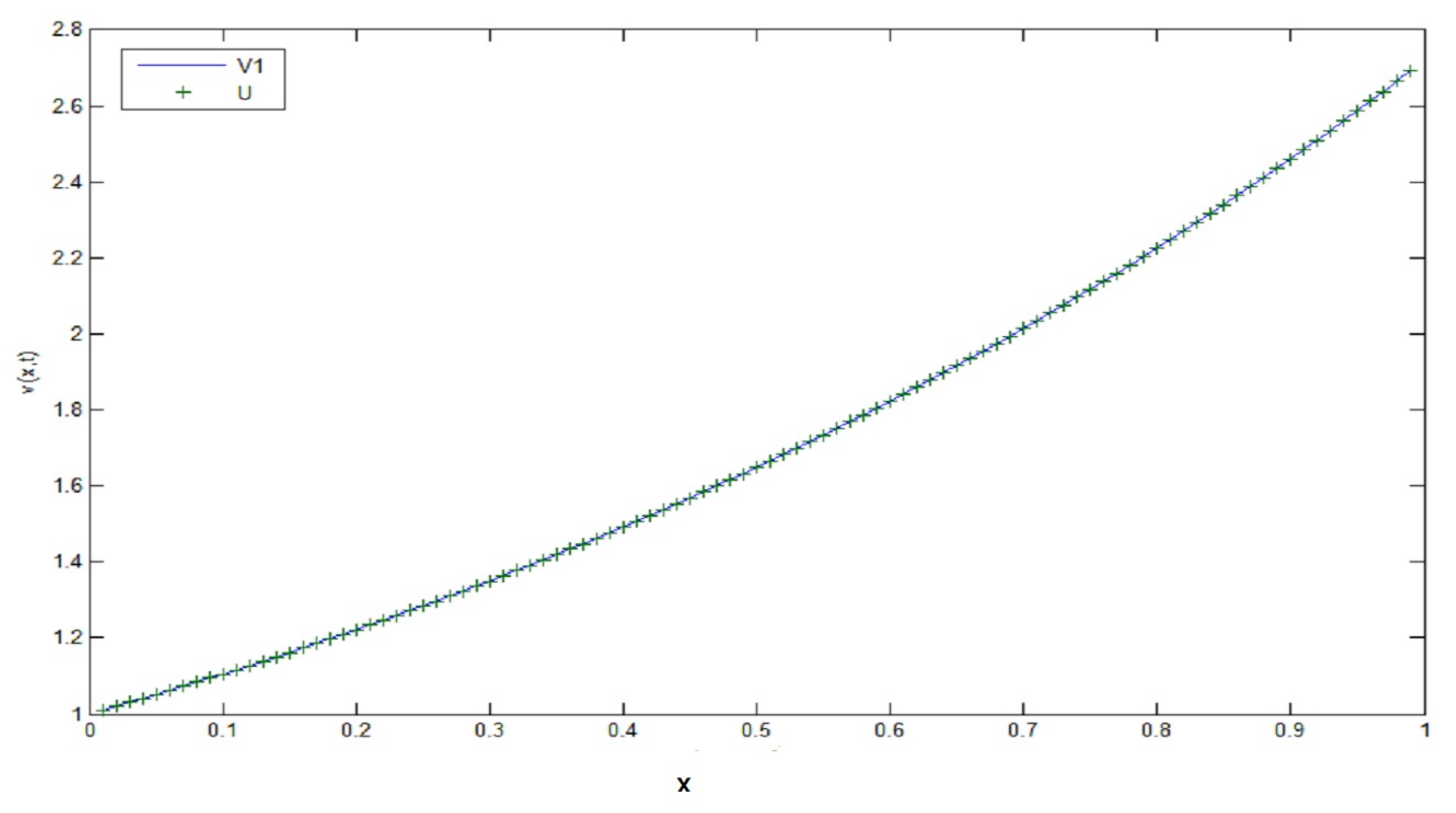
4.3. Applications

In this section, we give some numerical investigation tests.

Example 1.

We consider problems (4)–(6) with

$\alpha =\frac{3}{2},a(x,t)=-x-t,$

$b(x,t)=x+t,c\left(x\right)=2,g(x,t)=(\frac{3}{4}\sqrt{\pi }+2t\sqrt{t})e^x,\varphi \left(x\right)=\psi \left(x\right)=0,$

$\mu \left(t\right)=(e-1)t^{\frac{3}{2}},E\left(t\right)=t^{\frac{3}{2}}.$

The analytical solution is given by $v(x,t)=t^{\frac{3}{2}}{e}^x.$

The approximate solution $u(x,t)$ where A.E is the absolute error.

We see in Figure 1, Figure 2 and Figure 3 and

Table 1. $h=0.1;$$h_t=0.01$.

${\mathit{x}}_{\mathit{i}}$	${\mathit{u}}^1(\mathit{x},\mathit{t})$	${\mathit{v}}^1(\mathit{x},\mathit{t})$	$\mathbf{A}.\mathbf{E}$
$0.1$	$1.1052\times {10}^{-3}$	$1.3042\times {10}^{-3}$	$1.99\times {10}^{-4}$
$0.2$	$1.2214\times {10}^{-3}$	$1.4523\times {10}^{-3}$	$2.30\times {10}^{-4}$
$0.3$	$1.3499\times {10}^{-3}$	$1.6038\times {10}^{-3}$	$2.53\times {10}^{-4}$
$0.4$	$1.4918\times {10}^{-3}$	$1.7710\times {10}^{-3}$	$2.79\times {10}^{-4}$
$0.5$	$1.6487\times {10}^{-3}$	$1.9558\times {10}^{-3}$	$3.07\times {10}^{-4}$
$0.6$	$1.8221\times {10}^{-3}$	$2.1600\times {10}^{-3}$	$3.38\times {10}^{-4}$
$0.7$	$2.0138\times {10}^{-3}$	$2.3851\times {10}^{-3}$	$3.71\times {10}^{-4}$
$0.8$	$2.2255\times {10}^{-3}$	$2.6235\times {10}^{-3}$	$3.98\times {10}^{-4}$
$0.9$	$2.4596\times {10}^{-3}$	$2.7079\times {10}^{-3}$	$2.48\times {10}^{-4}$

,

Table 2. $h=0.1$, $h_t=0.001$.

${\mathit{x}}_{\mathit{i}}$	${\mathit{u}}^1(\mathit{x},\mathit{t})$	${\mathit{v}}^1(\mathit{x},\mathit{t})$	$\mathbf{A}.\mathbf{E}$
$0.1$	$3.4949\times {10}^{-5}$	$4.1175\times {10}^{-5}$	$6.23\times {10}^{-6}$
$0.2$	$3.8624\times {10}^{-5}$	$4.5515\times {10}^{-5}$	$6.89\times {10}^{-6}$
$0.3$	$4.2686\times {10}^{-5}$	$5.0301\times {10}^{-5}$	$7.61\times {10}^{-6}$
$0.4$	$4.7176\times {10}^{-5}$	$5.5590\times {10}^{-5}$	$8.41\times {10}^{-6}$
$0.5$	$5.2137\times {10}^{-5}$	$6.1435\times {10}^{-5}$	$9.30\times {10}^{-6}$
$0.6$	$5.7620\times {10}^{-5}$	$6.7895\times {10}^{-5}$	$1.03\times {10}^{-5}$
$0.7$	$6.3680\times {10}^{-5}$	$7.5034\times {10}^{-5}$	$1.14\times {10}^{-5}$
$0.8$	$7.0378\times {10}^{-5}$	$8.2923\times {10}^{-5}$	$1.25\times {10}^{-5}$
$0.9$	$7.7802\times {10}^{-5}$	$9.1415\times {10}^{-5}$	$1.36\times {10}^{-5}$

and

Table 3. $h=0.1,$$h_t=0.0001$.

${\mathit{x}}_{\mathit{i}}$	${\mathit{u}}^1(\mathit{x},\mathit{t})$	${\mathit{v}}^1(\mathit{x},\mathit{t})$	$\mathbf{A}.\mathbf{E}$
$0.1$	$1.1052\times {10}^{-6}$	$1.3020\times {10}^{-6}$	$1\times {10}^{-7}$
$0.2$	$1.2214\times {10}^{-6}$	$1.4389\times {10}^{-6}$	$2\times {10}^{-7}$
$0.3$	$1.3499\times {10}^{-6}$	$1.5903\times {10}^{-6}$	$2\times {10}^{-7}$
$0.4$	$1.4918\times {10}^{-6}$	$1.7575\times {10}^{-6}$	$2\times {10}^{-7}$
$0.5$	$1.6487\times {10}^{-6}$	$1.9424\times {10}^{-6}$	$2\times {10}^{-7}$
$0.6$	$1.8221\times {10}^{-6}$	$2.1466\times {10}^{-6}$	$3\times {10}^{-7}$
$0.7$	$2.0138\times {10}^{-6}$	$2.3724\times {10}^{-6}$	$3\times {10}^{-7}$
$0.8$	$2.2255\times {10}^{-6}$	$2.6219\times {10}^{-6}$	$3\times {10}^{-7}$
$0.9$	$2.4596\times {10}^{-6}$	$2.8974\times {10}^{-6}$	$4\times {10}^{-7}$

that the absolute error(A.E) gradually decreases when the step $h_t$ takes small values and getting very close to zero. That is, for $h_t=0.01$, $h_t=0.001$, and $h_t=0.0001$ the absolute error(A.E) decreases towards zero and the approximate solution tends towards the exact solution with the convergence order of $O(h+h_t).$

For $k=1$ (second iteration),

Table 4. $h=0.1,$$h_t={10}^{-2},{10}^{-3},{10}^{-5}$.

${\mathit{x}}_{\mathit{i}}$	${\mathit{h}}_{\mathit{t}}={10}^{-2}$	${\mathit{h}}_{\mathit{t}}={10}^{-3}$	${\mathit{h}}_{\mathit{t}}={10}^{-5}$
$0.1$	$1.84\times {10}^{-3}$	$5.80\times {10}^{-5}$	$5.80\times {10}^{-8}$
$0.2$	$1.74\times {10}^{-3}$	$5.45\times {10}^{-5}$	$5.45\times {10}^{-8}$
$0.3$	$1.62\times {10}^{-3}$	$5.06\times {10}^{-5}$	$5.06\times {10}^{-8}$
$0.4$	$1.49\times {10}^{-3}$	$4.63\times {10}^{-5}$	$4.63\times {10}^{-8}$
$0.5$	$1.33\times {10}^{-3}$	$4.15\times {10}^{-5}$	$4.16\times {10}^{-8}$
$0.6$	$1.17\times {10}^{-3}$	$3.63\times {10}^{-5}$	$3.63\times {10}^{-8}$
$0.7$	$9.82\times {10}^{-4}$	$3.05\times {10}^{-5}$	$3.05\times {10}^{-8}$
$0.8$	$7.40\times {10}^{-4}$	$2.40\times {10}^{-5}$	$2.41\times {10}^{-8}$
$0.9$	$1.26\times {10}^{-4}$	$1.64\times {10}^{-5}$	$1.69\times {10}^{-8}$

shows the absolute error decrease to zero and Figure 4, Figure 5 and Figure 6 show the approximate solution $u{}^2$ after two steps $2h_t$ tend towards the exact solution when $h_t$ close to zero, with convergence order $O(h+h_t).$

Remark 1.

For space step $h=0.01$ we find Figure A1 and Figure A2 in Appendix A.

Example 2.

We take: $\alpha =\frac{3}{2},a(x,t)=-x^2-t,b(x,t)=x-t,$

$c\left(x\right)=x+2t,g(x,t)=(4\sqrt{t}+{(t+1)}^2(x^2+2t)e^x,$$\Phi \left(x\right)=e^x;$

$\psi \left(x\right)=2e^x,\mu \left(t\right)={(t+1)}^2,E\left(t\right)={(t+1)}^2.$

The analytical solution of this problem is given by $v(x,t)={(t+1)}^2{e}^x.$

Table 5. $h=0.1,h_t={10}^{-2}$.

${\mathit{x}}_{\mathit{i}}$	$\mathbf{A}.\mathbf{E}$
$0.1$	$6.72\times {10}^{-4}$
$0.2$	$2.47\times {10}^{-3}$
$0.3$	$2.44\times {10}^{-3}$
$0.4$	$2.41\times {10}^{-3}$
$0.5$	$2.39\times {10}^{-3}$
$0.6$	$2.38\times {10}^{-3}$
$0.7$	$1.84\times {10}^{-3}$
$0.8$	$1.40\times {10}^{-2}$
$0.9$	$2.06\times {10}^{-1}$

,

Table 6. $h=0.1,h_t={10}^{-3}$.

${\mathit{x}}_{\mathit{i}}$	$\mathbf{A}.\mathbf{E}$
$0.1$	$1.22\times {10}^{-5}$
$0.2$	$4.28\times {10}^{-5}$
$0.3$	$4.24\times {10}^{-5}$
$0.4$	$4.20\times {10}^{-5}$
$0.5$	$4.15\times {10}^{-5}$
$0.6$	$4.10\times {10}^{-5}$
$0.7$	$4.03\times {10}^{-5}$
$0.8$	$4.83\times {10}^{-5}$
$0.9$	$5.48\times {10}^{-3}$

and

Table 7. $h=0.1$, $h_t={10}^{-4}$.

${\mathit{x}}_{\mathit{i}}$	$\mathbf{A}.\mathbf{E}$
$0.1$	$3.75\times {10}^{-7}$
$0.2$	$1.26\times {10}^{-6}$
$0.3$	$1.24\times {10}^{-6}$
$0.4$	$1.25\times {10}^{-6}$
$0.5$	$1.23\times {10}^{-6}$
$0.6$	$1.22\times {10}^{-6}$
$0.7$	$1.20\times {10}^{-6}$
$0.8$	$1.19\times {10}^{-6}$
$0.9$	$1.72\times {10}^{-4}$

show the values of the absolute error.

In this example from Table 5, Table 6 and Table 7 and Figure 7, Figure 8 and Figure 9 we see again for space step $h=0.1$ the absolute error tends to zero when the time step $h_t$$({10}^{-2},$${10}^{-3},$${10}^{-4})$ takes a value close to zero, with convergence order $O(h+h_t).$ In Figure 9 we take into account x $\in \left[0.8965,0.9000\right]$ to see the variation of error because it is very close to zero when x $\in \left[0.1,0.8\right].$

Remark 2.

For the space step $h=0.01$ we find Figure A3, Figure A4, Figure A5 in Appendix A.

Table 8. $h=0.1$.

	Value  of  ${\mathit{h}}_{\mathit{t}}$	${10}^{-3}$	${10}^{-5}$	${10}^{-7}$
${∥E^1∥}_{\infty }$ for	$\alpha =1.2$	$9.5736$×${10}^{-4}$	$1.3196\times {10}^{-6}$	$5.2768\times {10}^{-9}$
	$\alpha =1.4$	$1.1294\times {10}^{-4}$	$1.2671\times {10}^{-7}$	$2.0154\times {10}^{-10}$
	$\alpha =1.6$	$2.3162\times {10}^{-5}$	$1.2692\times {10}^{-8}$	$7.9794\times {10}^{-12}$
	$\alpha =1.8$	$1.53\times {10}^{-4}$	$1.4449\times {10}^{-9}$	$3.4062\times {10}^{-13}$
	$\alpha =1.9$	$4.7963\times {10}^{-6}$	$6.2306\times {10}^{-10}$	$8.6153\times {10}^{-14}$

shows the error norm ${∥E^k∥}_{\infty }$ for different values of $\alpha$ defined by

$${∥E^k∥}_{\infty }=\underset{1\le i\le N-1}{max}\left|e_i\right|,\mathrm{where}{E}^k=V{}^k-U{}^k={\left(e_1^k,\dots ,e_{N-1}^k\right)}^T$$

We see in Table 8, for the space step $h=0.1$, and for the different values of $\alpha$, the error keeps the same behavior; that is, the error norm tends towards zero when the time step $h_t$ takes values close to zero, with an order of convergence $O(h+h_t)$. For $\alpha =1.2$ (value close to 1) the error is greater compared to the case $\alpha =1.9$ (value close to 2) due of the fractional operator being approximated by the formula called $L_2.$

5. Conclusions

In this paper, the existence and uniqueness of the solution of a Caputo time fractional problem with nonhomogeneous boundary integral conditions are established. We use the “energy inequality” method which is an efficient functional analysis method.

For the numerical study, these kinds of boundary conditions have been applied for the first time to such problems, where we combined the finite difference method with the numerical integration to obtain the approximate solution. The results obtained by this technique are very encouraging from the point of view that the numerical schemes are stable and convergent.

As further research directions, we aim at studying the same problem using the compact finite difference method in order to obtain more precise results, change the sense of fractional derivatives and/or extend the study to time–space fractional derivatives.

References

- Mainardi, F. Fractional diffusive waves in viscoelastic solids. Nonlinear Waves Solids 1995, 137, 93–97. [Google Scholar]
- Podlubny, I. Fractional Differential Equations; Academic Press: San Diego, CA, USA, 1999. [Google Scholar]
- He, J.H. Approximate analytical solution for seepage flow with fractional derivatives in porous media. Comput. Methods Appl. Mech. Eng. 1998, 167, 57–68. [Google Scholar] [CrossRef]
- Kilbas, A.A.; Srivastava, H.M.; Trujillo, J.J. Theory and Applications of Fractional Differential Equations; Elsevier: Amsterdam, The Netherlands, 2006. [Google Scholar]
- Alikhanov, A.A. Boundary value problems for the di usion equation of the variable order in differential and difference settings. Appl. Math. Comput. 2012, 219, 3938–3946. [Google Scholar]
- Li, X.J.; Xu, C.J. Existence and uniqueness of the weak solution of the space-time fractional diffusion equation and a spectral method approximation. Commun. Comput. Phys. 2010, 8, 1016–1051. [Google Scholar]
- Smit, W.; de Vries, H. Rheological models containing fractional derivatives. Rheol. Acta 1970, 9, 525–534. [Google Scholar] [CrossRef]
- Monje, C.A.; Chen, Y.; Vinagre, B.M.; Xue, D.; Feliu, V. Fractional-Order Systems and Controls: Fundamentals and Applications; Springer: London, UK, 2010. [Google Scholar]
- Enacheanu, O. Fractal Modeling of Electrical Networks. Ph.D. Thesis, Joseph Fourier University, Grenoble, France, October 2008; pp. 47–53. [Google Scholar]
- Kaufmann, E.R.; Mboumi, E. Positive solutions of a boundary value problem for a nonlinear. fractional differential equation. Electron. J. Qual. Theory Differ. Equ. 2007, 3, 1–11. [Google Scholar] [CrossRef]
- Furati, K.M.; Tatar, N. An existence result for a nonlocal fractional differential problem. J. Fract. Calc. 2004, 26, 43–51. [Google Scholar]
- Mesloub, S. Existence and uniqueness results for a fractional two-times evolution problem with constraints of purely integral type. Math. Methods Appl. Sci. 2016, 39, 1558–1567. [Google Scholar] [CrossRef]
- Sosnovskii, L.A.; Komissarov, V.V.; Shcherbakov, S.S. A Method of Experimental Study of Friction in a Active System. J. Frict. Wear 2012, 33, 174–184. [Google Scholar] [CrossRef]
- Shcherbakov, S.S. State of volumetric damage of tribo-fatigue systeme. Strength Mater. 2013, 45, 171–178. [Google Scholar] [CrossRef]
- He, C.; Liu, J.; Wang, W.; Liu, Q. The Tribo-Fatigue Damage Transition and Mapping for Wheel Material under Rolling-Sliding Contact Condition. Materials 2019, 12, 4138. [Google Scholar] [CrossRef] [Green Version]
- Day, W.A. A decreasing property of solutions of parabolic equations with applications to thermoelasticity. Quart. Appl. Math. 1983, 40, 319–330. [Google Scholar] [CrossRef] [Green Version]
- Anguraj, A.; Karthikeyan, P. Existence of solutions for fractional semilinear evolution boundary value problem. Commun. Appl. Anal. 2010, 14, 505–514. [Google Scholar]
- Jesus, M.-V.; Ahcene, M. Existence, uniqueness and numerical solution of a fractional PDE with integral conditions. Nonlinear Anal. Model. Control 2019, 24, 368–386. [Google Scholar]
- Benchohra, M.; Graef, J.R.; Hamani, S. Existence results for boundary value problems with nonlinear fractional differential equations. Appl. Anal. 2008, 87, 851–863. [Google Scholar] [CrossRef]
- Daftardar-Gejji, V.; Jafari, H. Boundary value problems for fractional diffusion-wave equation. Aust. J. Math. Anal. Appl. 2006, 3, 1–8. [Google Scholar]
- Alikhanov, A.A. On the stability and convergence of nonlocal difference schemes. Differ. Equ. 2010, 46, 949–961. [Google Scholar] [CrossRef]
- Alikhanov, A.A. A new difference scheme for the time fractional diffusion equation. J. Comput. Phys. 2015, 280, 424–438. [Google Scholar] [CrossRef] [Green Version]
- Alikhanov, A.A. Stability and convergence of difference schemes for boundary value problems for the fractional-order diffusion equation. Comput. Math. Math. Phys. 2016, 56, 561–575. [Google Scholar] [CrossRef]
- Meerschaert, M.M.; Tadjeran, C. Finite difference approximations for fractional advection dispersion flow equations. J. Comput. Appl. Math. 2004, 172, 65–77. [Google Scholar] [CrossRef] [Green Version]
- Shen, S.; Liu, F. Error analysis of an explicit finite difference approximation for the space fractional diffusion. Anziam J. 2005, 46, C871–C887. [Google Scholar] [CrossRef] [Green Version]
- El-Nabulsi, R.A. Finite Two-Point Space without Quantization on Noncommutative Space from a Generalized Fractional Integral Operator. Complex Anal. Oper. Theory 2018, 12, 1609–1616. [Google Scholar] [CrossRef]
- El-Nabulsi, R.A. The fractional Boltzmann transport equation. Comput. Math. Appl. 2011, 62, 1568–1575. [Google Scholar] [CrossRef] [Green Version]
- El-Nabulsi, R.A. Nonlocal-in-time kinetic energy in nonconservative fractional systems, disordered dynamics, jerk and snap and oscillatory motions in the rotating fluid tube. Int. J. Non-Linear Mech. 2017, 93, 65. [Google Scholar] [CrossRef]
- Yan, B.H.; Yu, L.; Yang, Y.H. Study of oscillating flow in rolling motion with the fractional derivative Maxwell model. Prog. Nucl. Energy 2011, 53, 132–138. [Google Scholar] [CrossRef]
- Li, X.; Yang, X.; Zhang, Y. Error estimates of mixed finite element methods for timefractional Navier-Stokes equations. J. Sci. Comput. 2017, 70, 500–515. [Google Scholar] [CrossRef]
- Yildirim, A. Analytical approach to fractional partial differential equations in fluid mechanics by means of the homotopy perturbation method. Int. J. Numer. Methods Heat Fluid Flow 2010, 20, 186–200. [Google Scholar] [CrossRef]
- Zhou, Y.; Peng, L. On the time-fractional Navier–Stokes equations. Comput. Math. Appl. 2017, 73, 874–891. [Google Scholar] [CrossRef]
- Yu, B.; Jiang, X.Y.; Xu, H.Y. A novel compact numerical method for solving the two-dimensional non-linear fractional reaction-subdiffusion equation. Numer. Algorithms 2015, 68, 923–950. [Google Scholar] [CrossRef]
- Povstenko, Y. Linear Fractional Diffusion-Wave Equation for Scientists and Engineers; Springer: Berlin/Heidelberg, Germany, 2010. [Google Scholar]
- Oussaeif, T.-E.; Bouziani, A. Existence and uniqueness of solutions to parabolic fractional differential equations with integral conditions. Electron. J. Differ. Equ. 2014, 2014, 1–10. [Google Scholar]